Publisher’s version / Version de l'éditeur:
ASHRAE Transactions, 96, 1, pp. 590-598, 1990
READ THESE TERMS AND CONDITIONS CAREFULLY BEFORE USING THIS WEBSITE. https://nrc-publications.canada.ca/eng/copyright
Vous avez des questions? Nous pouvons vous aider. Pour communiquer directement avec un auteur, consultez la première page de la revue dans laquelle son article a été publié afin de trouver ses coordonnées. Si vous n’arrivez pas à les repérer, communiquez avec nous à [email protected].
Questions? Contact the NRC Publications Archive team at
[email protected]. If you wish to email the authors directly, please see the first page of the publication for their contact information.
NRC Publications Archive
Archives des publications du CNRC
This publication could be one of several versions: author’s original, accepted manuscript or the publisher’s version. / La version de cette publication peut être l’une des suivantes : la version prépublication de l’auteur, la version acceptée du manuscrit ou la version de l’éditeur.
Access and use of this website and the material on it are subject to the Terms and Conditions set forth at
Multiple tracer gas techniques for measuring interzonal airflows for
three interconnected spaces
Enai, M.; Shaw, C. Y.; Reardon, J. T.; Magee, R. J.
https://publications-cnrc.canada.ca/fra/droits
L’accès à ce site Web et l’utilisation de son contenu sont assujettis aux conditions présentées dans le site LISEZ CES CONDITIONS ATTENTIVEMENT AVANT D’UTILISER CE SITE WEB.
NRC Publications Record / Notice d'Archives des publications de CNRC:
https://nrc-publications.canada.ca/eng/view/object/?id=7e5ab596-d3e4-4d53-a59f-8109683f6998 https://publications-cnrc.canada.ca/fra/voir/objet/?id=7e5ab596-d3e4-4d53-a59f-8109683f6998
Ser
TH
1
N21d
National Research
Condl
national
no.1652
c.2
ouncil Canada
de recherdres
Canada
BLDG,
Institute for
lnstitut de
-
Research in
recherche en
Construction
construction
Multiple 'Tracer Gas Techniques for
Measuring lntenonal Airtlo ws for
Three Interconnected Spaces
by
M. Enai, C.Y. Shaw, J.T. Reardon and R.J. Magee
Reprinted from
ASHRAE Transactions
1990
Vol. 96, Pt.
1,8
p.
(IRC Paper No. 1652)
-
NRCC
3171
1
NRC
-
ClSTl7
I R C
L I B R A R Y
*La .meth-ode des gaz traceurs multiples est souvent utilisee pour prbvoir les
Gcoulements d'air interzonaux dans les batiments.
Dans une etude
antkrieure, cette mkthode a tit6 appliquk
h
un espace compost5 de deux locaux
csmmuniquants oQ les 4coulements d'air
h
travers le mur mitoyen ont btk
rkglbs et mesurb. Les rksultats ont revel& que les bcoulements calsulbs B
partir de diffhrents ensembles de concentrations de gaz traceurs mesures
simultankment (obtenus h diffbrents temps d'kchantillonnage au cours d'un
essai) n'etaient pas toujours les memes. Des lignes directrices s'imposent
donc pour faciliter le choix d'ensembles de concentrations de gaz traceurs
appropries ( B partir des mesures) pour la mkthode des gaz traceurs multiples.
Dans la prbsente etude, les locaux d'essai ont etk port&
A
trois pieces
communicantes.
Une mbthode a kt6 mise au point pour dkterminer
l'ensemble de concentv-
-
'-"coulement d'air
interzonal. La mktho
et les rkultats
MULTIPLE TRACER GAS TECHNIQUES FOR
MEASURING INTERZONAL AIRFLOWS
FOR THREE INTERCONNECTED SPACES
M. Enai
C.Y. Shaw
J.T. Reardon
R.J. Magee
ABSTRACT
The multiple tracer gas method is often used to predict interzonal airflows in buildings. In a previous study, this method was applied to a space consisting of two interconnected rooms where the airflows through the common wall were controlled and measured. The results indicated that the predicted airfows based on dif- ferent sets of simultaneously measured tracer gas con- centrations (obtained at different sampling times during a test) were not always the same. Guidelines are, there- fore, needed to facilitate the selection of the appropriate set of tracer gas concentrations (from the measure- ments) for use with the multiple tracer gas method.
In this study, the test rooms were expanded to three interconnected rooms. A method was developed to deter- mine the appropriate set of concentrations for interzonal airflow calculations. The proposed method was tested in the laboratory and the results are discussed.
INTRODUCTION
As concern for indoor air quality has grown, so too has the need to measure interzonal airflows to assess the distribution of outdoor air in buildings. These airflows can be evaluated using the multiple tracer gas method (Sinden 1978; Sherman et al. 1980; I'Anson et al. 1982; Perera 1983). It involves the injection of a different tracer gas into each of several interconnected spaces and the measurement of the tracer gas concentrations as a func- tion of time. Based' on the simultaneously measured tracer gas concentrations, the interzonal airflows can then be calculated from the mass conservation equa- tions for each tracer gas and the mass flow balance equations for the air.
The application of the method is not straightforward, even for the simplest case, e.g., a building consisting of two interconnected chambers. In a previous study (Enai et al. 1990), the multiple tracer gas method was applied to a space consisting of two interconnected rooms where the airflows between the two rooms were controlled and measured. Two test procedures were used to introduce the tracer gases into the rooms: the decay technique for both rooms, and constant injection for one room and
decay for the other room. The results indicated that, for any given test, the calculated airflow rates based on different sets of concentrations (measured at different times during a test) were not always the same and that the agreement between the calculated and measured air- flow rates generally worsened when the concentrations used were measured earlier than 30 minutes after injec- tion or later than 70 minutes after injection. These findings suggest that to achieve the best result, some guidelines are required for selection of the appropriate set of con- centrations for calc'ulating the interzonal airflows. A method was derived for calculating interzonal airflows for two interconnected rooms.
In this study, the test facility was expanded to three interconnected rooms, where the airflows between any two rooms were controlled at constant rates and mea- sured during the experiments. The main objectives of the study were (1) to determine the appropriate set of con- centrations that can be used for interzonal airflow calcu- lations and (2) to determine the accuracy of the multiple tracer gas technique under laboratory conditions.
GOVERNING EQUATIONS
Figure 1 shows the case of three interconnected zones. If three tracer gases, denoted by A, 6, and C, are injected into the zones (one for each zone), the rates of change in tracer gas concentrations in the three zones can be described by the following equations, assuming that the tracer gas concentrations outside the zones are negligible:
M. Enai, Associate Professor, Architectural Department, Hokkaido University; C.Y.
Shaw,
J.T. Reardon, and R.3. Magee, Institute for Research in Construction, National Research Council, Canada.THIS PREPRINT IS FOR DISCUSSION PURPOSES ONLY, FOR INCLUSION IN ASHRAE TRANSACTIONS 1990. V. 96, Pt. 1. Not to be reprinted in whole cr in part wlthout wrltten permission of the Amerlcan Society of Heating, Refrigerating and Air-Conditioning Engineers. Inc.. 1791 Tullie Circle, NE, Atlanta. GA 30329. Opinions, findings, conclus~ons, or recommendations expressed in this paper are those of the author(s) and do not necessarily reflect the views of ASHRAE.
Flgure 1 Test rooms
V2( dC62/dt) = F1 2
*
C B ~ - ( F20 + F2 1 + F23) Cm+ F 3 2 * C m + Qm (5)
V2( dCc2/dt) = F12
*
CC1 - (FpO + F21+
F23)CC2+ F32
*
cC3 (6) V3(dCA3/dt) = F13*
CAI+
F23*
CA2- ( F30 + F31 + F 3 2 ) c ~ 3 ( 7 ) V3(dCmldt) = F13
*
CB1 +*
CB2- ( F30 + F31 + F 3 2 ) c ~ (8)' V3(dCc3/dt) = F13
*
Ccl+
F23*
CC2- ( F30 + F31 + F 3 2 ) C ~ 3 +QCJ (9)
The mass flow balance equations for the three zones are: - (F1O + F12 + F13) + FO1 + F21 + F31 = 0 ( I 0 )
- (F20 + F21 + F23) + F02 + F12 + F3, = 0 ( I 1 )
- (F30 + F31 + F32) + F03 + F23 + F13 = 0 ( I 2 ) where
V = room volume
C = tracer gas concentration t = time
F,, = airflow rate from zone i to zone j
Q = tracer gas release rate
1
Fzo
'0 20 40 60 80 100 120 140 160
ELAPSED TIME, rnin
F02
Y
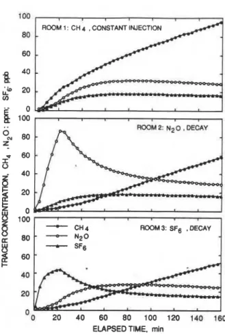
Figure 2 Typical tracer gas concentration profiles
y Fo3 ROOM 2 F a 2 4
-
' 2 3 TEST METHODSThe test zones, as shown in Figure 1 , were three interconnected rooms in a laboratory-office building. Rooms 1 and 2 were each 4.8 m wide, 4.8 m long, and
2.87 m high, and Room 3 was 2.33 m wide, 1 1 m long, and 2.57 m high. The walls, doors, and ceilings of the rooms were sealed to minimize air leakage. Each con- necting doorway was sealed with plywood panels through which two airflow systems were installed (one for each flow direction). The airflow systems consisted of a fan, an airflow measuring device, and an airflow controller. Each individual airflow was controlled at a constant rate and continuously measured throughout each test. Except for those through the airflow systems,
l
F12The subscripts 0 , 1, 2 , and 3 denote the outside and zones 1 , 2, and 3, respectively, and A, B, and C I ROOM 3
refer to the tracer gases used. As an example, Flo rep- resents the airflow from Zone 1 to the outside, and CAl is the concentration of tracer gas A in Zone 1 .
If three tracer gases, A, B, and C, are injected into Zones 1 , 2, and 3, respectively, and their concentrations in each room are monitored over time, the 12 unknowns
- F,o, F12, F,,, Fol, F 2 ~ , F2,, F23, Fo2, F3,, F3,, F32, and Fo3
- can be evaluated by solving Equations 1 through 12 simultaneously. Similarly, if all the airflow rates are known, they can be used in the solutions to the above set of simultaneous differential equations to calculate the tracer gas concentration profiles.
I
F2l
v
'37 r
TABLE 1
Test Conditions
Injection Mode(*) Interzonal Airflows, ach
Test No. Rm.1 Rm.2 Rm.3 6 2 F~ 3 F21 F23 F 3 ~ F32 101 D D D 0.79 0,79 0.80 0 79 0.80 0.78 102 D 1(87) l(93) 0.80 0,80 0.80 0.80 0.77 0.80 103 D C l(94) 0.79 0.80 0.80 0.80 0.78 0.80 104 D D D 0.50 0.48 0,51 0.51 0.49 0.49 105 1(55) D D 0.50 0,48 0.51 0 47 0.49 0.50 106 1(78) D D 1-00 0.23 0.25 0,98 0.98 0.24 107 l(63) D D 0.30 0.90 0.61 0.51 0 61 0.79 108 D D D 0.30 0.89 0.60 0.51 0.60 0.79 109 D D D 1-00 0.23 0 25 0 99 0 98 0 26 110 1(26) D D 0.25 0.24 0.25 0.23 0.25 0 24 111 D D D 0.25 0 24 0 25 0 24 0.25 0 24 112 l(94) D D 0.79 0.79 0.80 0.79 0.80 0 79 113 D D D 0 78 0.79 0.79 0.78 0.77 0.80 114 1(71) D D 0.78 0.60 0.40 0.70 0.99 0 31
'C, D, and I denote constant concentratton, decay, and constant ~nlect~on, respect~vely (values In brackets are the injection rates of pure gas, mL1mln). the air leakage rates between the test rooms and their
surroundings were not measured.
The tracer gas injection tube was located at the center of each room. The rooms were each divided into eight volumetrically equal regions with a sampling tube installed at the center of each region. Mixing of tracer gas in the test rooms has been studied previously (Enai et al. 1990). Based on the results, the sampling tubes in each room were connected to a manifold to produce an "average" sample.
Each test began by adjusting the airflows ~n the six systems to rates between 0.2 to 1 air change per hour (ach). Then, CH,, SF,, and N,O were simultaneously introduced into Rooms 1, 2, and 3 , respectively. Imme- diately after injection, the concentrations of the three gases at the manifolds in each room were measured at four-minute intervals for a period of two to five hours. TEST RESULTS
Fourteen multiple tracer gas tests were conducted. The test conditions are listed in Table 1. Figure 2 shows a typical set of concentration profiles measured in the test rooms. Each set consists of nine profiles, one for each tracer gas in each room. From such profiles, the concentrations of CH,, SF,, and N20 at about 30 minutes after injection of the tracer gases were used to calculate
F,,, FZ1, F13, F3,, F23, and F3, from Equations 1 through
12. Similar calculations were made using subsequent sets of concentration values measured at four-minute intervals for about one-and-a-half hours. These calcula- tions were carried out for all tests.
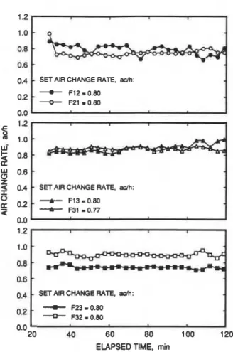
To examine the effect of injection techniques on the calculated airflow rates, four tests using different combi- nations of tracer gas injection techniques and uniform interzonal airflow settings were conducted. The airflows of these tests were all set at about 0.8 ach. The combinations of injection techniques were (a) decay in all three rooms; (b) decay in Room 1 and constant injection in Rooms 2 and 3; (c) decay in Room 1, constant concentration in Room 2, and constant injection in Room 3; and (d) con- stant injection in Room 1 and decay in Rooms 2 and 3. Figures 3, 4, 5, and 6 show the calculated interzonal
airflow rates as functions of time for these four tests. Tne results indicate that:
1. For the same test, the calculated airflow rates based on different sets of concentrations (measured at different times) were not always the same.
2. The calculated airflow rates, based on the con- centrations measured between 30 and 70 minutes after injection, agreed with the measurement within 25% of the measured rates.
3. No clear evidence was found to suggest that the technique used to inject tracer gases (e.g., decay, constant injection, or constant concentration) has a sig- nificant or systematic effect on the calculated results. However, in some cases where the decay technique was used to inject tracer gases into more than one room, the agreement between the calculated and mea- sured airflow rates worsened after 70 minutes.
These conclusions are not restricted to cases with uniform interzonal airflow settings. Similar behavior in the calculated results was observed for tests with nonuniform interzonal airflows.These findings suggest that concen- trations selected from only a certain portion of the mea- sured profiles can give a good Bstimate of interzonal airflows, as had been observed for the case of two inter- connected rooms (Enai et al. 1990). To determine the appropriate set of concentrations for calculating inter- zonal airflows, the following method is proposed. METHOD FOR CALCULATING
INTERZONAL AIRFLOWS
Figures 3 through 6 show that the calculated inter- zonal airflow rates based on different sets of concentrations are not always the same, and a method of determining the appropriate set for use in calculations is needed.
Equations 1 through 9 define the tracer gas con- centration profiles for a typical case of three intercon- nected zones. If all the airflows for such a case are known, the tracer gas concentration profiles can be cal- culated explicitly from these equations. The approach proposed here, therefore, is to estimate the airflow rates using a set of concentrations measured at some arbi- trary time. These airflows are then used to estimate the
SET AIR CHANGE RATE, am:
-
F12-0.790.2
20 40 60 80 100 120
ELAPSED TIME, min
Figure 3 Calculated interzonal airflow rates case (a) Room 1: decay, Room 2: decay, and Room 3: decay
concentrations for a later time, using equations derived from Equations 1 through 9 (see Tracer Gas Concentra- tion Profiles section). These estimated concentrations are then compared with the corresponding measured concentrations and, if the agreement is not satisfactory, the procedure is repeated with a set of concentrations measured at a later time. This comparison is made for concentrations at two different times, five sampling inter- vals apart, to ensure that the agreement between the calculated and measured concentration profiles is not accidental (e.g., the two profiles cross each other at one time but do not agree in general). The final calculated airflow rates are achieved when satisfactory agreement between the measured and calculated concentrations is reached at the two points (see Procedures for Calcu- lating Interzonal Airflows section).
Tracer Gas Concentration Profiles
The concentration profiles of each tracer gas are defined by three equations, one for each room. Of the three equations, only one has a source term (e.g., QAl in Equation 1). Only one general solution to the three-equa- tion set need be found for a single tracer gas, since the same solution will apply to the other two tracer gases. By dropping the subscript A and letting
Nl = (F10 + F12 + F13)IVl
SET AIR CHANGE RATE, adh:
SET AIR CHANGE RATE, aclh:
-+
F13 -0.80*
F31-
0.7720 40 60 80 100 120
ELAPSED TIME, min
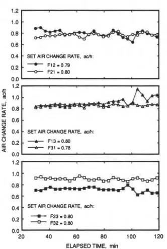
Figure 4 Calculated interzonal airflow rates case (b) Room 1: decay, Room 2: constant injection, and Room 3: constant injection
N3 = (F30 + F31 + F32)lV3
Equations 1 , 4 , and 7 become the set of three gen- eral equations:
From Equations 13,14, and 15, it can be shown that the differential equation for the gas concentration profile Cl is
SET AIR CHANGE RATE, ach:
+
F13=0.80*
F31 = 0.78SET AIR CHANGE RATE, ach:
ELAPSED TIME, min
Figure 5 Calculated interzonal airflow rates case (c)
Room 1: decay, Room 2: constant concentration, and Room 3: constant injection
Since all the coefficients but one (for Q1lVl) in Equation 16 are common to the corresponding equa- tions for C2 and C3, the general differential equation for the three tracer gas concentration profiles, C,, where i
= 1, 2, and 3, is
where
The solution to Ci can be obtained by the Laplace transformation method (see Appendix A). Thus,
0.4
-
SET AIR CHANGE RATE, adh: 0 2-
*
F12-
0.79 F21-
0.80 0.0 1.2 r3
1 . 0 - ui5
0.8;
b
0.60.4
-
SET AIR CHANGE RATE. adh:0.4
1
SET AIR CHANGE RATE, acm:\
4
V.U - -
20 40 60 80 100 120
ELAPSED TIME, min
Figure 6 Calculated interzonal airflow rates case (d)
Room 1: constant injection, Room 2: decay, and Room 3: decay
In the above equation, C,(t) is the tracer gas con- centration in Room iat time t where i = 1, 2, and 3. The coefficients are xi = -{[(N2
-
a)*
(N3-
a)-
(F3dV3)*
(F2dv2)1*
Cl(O) + [(N3-
a)* (F2lIVl)
+ (F2dVl)*
(F3llv3)l* c2(o)
+ [(N2 - a)*
(F31lVi) + (F2,lVl)*
(F32lV2)l" C3(0) + (N2+ N3-a)*
(Q1/Vl) +Kdllall[(c- a)*
( a - b)lX2 = -([(N3 - a) $: (F12/V2)
+
(F13/V2)*
( F32/V3)]*
Cl(0) + [(Nl -a)*(N3-a)-(F31/V3)*
(Fl3/Vl)1*
C2(0) + [(N1 - a)*
(F3~IV2) + (F121V1)*
(F31/V2)1*
C3(0) + (F121V1)*
(Ql/V2)+
K,latl[(c- a)*
( a - b)] Y2 = -([( N3 - b) :!: (F121V2)+
(F1$V2) (F321V3)]*:
C1(0)+
[(N1 - b)*
(N3 - b) - (F3,/V3)*
(Fi3/Vi)1*
C2(0) + [(Ni - b)*
(F321V2) + (F12/v1)*
(F3i/vz)]*
c3(0) + (F12/v1)* (Q1/V2)
+
Kd2/btl[(a- b)*
( b - c)]Z2 = -([(N, - c)
*
(FidV2) + (FidVz)*
(F3zIv3)l*
C1(0)+
[(Nl - C)*
(N3 - C) - (F3,1V3) *(F13lVl)l*
C2(0) + [(Nl -c)*(F32lV,)+ (F12lVl)
*
(F3llV2)l*
C3(0) + (F12lVl)*
(Q1lVl)+
K,lctl[(b- c)*
( c - a)]X3 = -1[(N2 - a)
*
(FidV3) + (Fi2IV3) * (F2dV2)I*
cl(o) + [(N1 -a)*
(F2dV3) + (FldVl)*
(F21lV3)I*
C2(0) + [(N1 - a)*
(N2 - a) - (F211V2)*
(F12lVl)l*
C3(0) + (FldVl)*
(Q1/V3)+ KdJ/atI[(c
- a)*
(a - b)] z3= -([(N2 - c)*
(Fidv3) + (Fi2lv3)*
(F2dV2)l*
c ~ ( O ) + [ ( ~ l - c )*
(F2dV3) + (FldVI)*
(F2i/V3)1*
C2(0) + [(Ni - c)*
(N2 - C) - (F211V2) ;"Fi2/vi)]*
c3(0) + (Fidvi)*
(Q1/V3)+
KdJIc]I[(b- C)*
( c - a)]Similar equations for concentration profiles under decay condition only have been derived by Irwin and Edwards (1987).
Procedures for Calculating Interzonal Airflows
The following procedures are proposed for calcu- lating interzonal airflows:
(a) Let t = t,. Since it normally takes more than 30 minutes to achieve adequate mixing, t, should not be less than 30 minutes.
(b) Calculate the corresponding interzonal airflows from Equations 1 through 12 using the nine concentra- tions (one for each gas in each room).
(c) Calculate the concentrations C, (where i = 1, 2, and 3) at Ti where Ti = t
+
Dt (Dt is one sampling inter- val; four minutes was used in this study) from Equation18 using the interzonal airflows obtained in (b).
0.0 0.2 0.4 0.6 0.8 1.0 1.2
MEASURED INTERZONAL AIR FLOW, adh
Figure 7 Comparison of measured and calculated airflow rates in test rooms
(d) Compare the calculated C,values with the val- ues for C, measured at Ti.
(e) If the calculated and measured values do not agree within a preset criterion (e.g., 2% was used in this study; a more lenient criterion may be needed for field tests), let
t =
t+ Dtand repeat the procedures starting at (b).(f) Otherwise, calculate C, at T2 where T2 =
t
+
5*
Dt and compare these with the corresponding mea- sured values.
(g) If the calculated and measured values do not agree within a preset criterion (e.g., 2% was used in this study; a more lenient criterion may be needed for field tests), let
t
= t + Dt and repeat the procedures startingat (b).
(h) Otherwise, the airflows used are the calculated airflows. A computer program has been developed for calculating interzonal airflows for three-room systems, which can accommodate any combination of tracer gas injection techniques used in this study.
COMPARISON BETWEEN CALCULATED AND MEASURED AIRFLOWS
The calculated and measured values for F12, F2,, F13, F3i, F23, and F3, are given in Table 2 and Figure 7.
Also included in Table 2 are the values of tat which the concentrations were selected for the calculated inter- zonal airflows. As shown in Table 2, the values of twere between 32.5 to 70.8 minutes, depending on the test conditions.
The standard errors of estimate were calculated for two different tracer gas injection techniques: (a) decay in all three rooms and (b) constant injection in one room and decay in the remaining rooms (other com- binations of injection techniques were not considered due to limited data). They are 0.065 and 0.054 ach for cases (a) and (b), respectively, suggesting that neither injection technique appears to have a significant advan- tage over the other in terms of the accuracy of interzonal airflow calculations. Figure 7 and Table 2 show that the calculated and measured airflow rates agreed within 20% (of the measured value).
TABLE 2
Calculated and Measured Airflow Rates
Interzonal Airflows, ach Run
Test Result Time
NO. F12 F~ 3 F21 F z 3 F 3 ~ F3z (min) 101 Measured 0.79 0 79 0.80 0.79 0.80 0.78 Calculated 0.86 0.76 0.80 0.65 0.92 0.88 33.2 - 102 Measured 0.80 0 80 0.80 0.80 0.77 0.80 Calculated 0.89 0.82 0 74 0.74 0.90 0.92 32.5 103 Measured 0.79 0.80 0 80 0,80 0.78 0.80 Calculated 0.81 0.87 0.70 0,74 0.82 0.93 65.5
1
104 Measured 0.50 0,48 0.51 0.51 0.49 0.49 Calculated 0.54 0,55 0 48 0.46 0.56 0.53 40.41.
105 Measured 0.50 0.48 0 51 0 47 0.49 0.50 Calculated 0.48 0.50 0 44 0.45 0.52 0 58 56.8 106 Measured 1 .OO 0 23 0.25 0.98 0.98 0.24 Calculated 1 06 0.25 0 23 0.92 1.03 0.27 42.9 107 Measured 0 30 0.90 0.61 0.51 0.61 0.79 Calculated 0.36 0.91 0 57 0.45 0.67 0.86 40.7 108 Measured 0 30 0.89 0 60 0.51 0.60 0.79 Calculated 0.36 0.84 0 55 0.46 0.68 0 85 37.3 109 Measured 1 .OO 0.23 0 25 0 99 0.98 0.26 Calculated 1.06 0 22 0.23 0.93 1.06 0.31 47.7 110 Measured 0.25 0.24 0.25 0.23 0 25 0.24 Calculated 0 24 0 22 0,23 0.20 0 30 0.28 70.8 I t 1 Measured 0.25 0.24 0.25 0 24 0.25 0.24 Calculated 0.25 0.23 0.23 0.19 0 29 0.31 32.5 112 Measured 0.79 0.79 0 80 0.79 0 80 0.79 Calculated 0 83 0.78 0.80 0.67 0.82 0.87 50.1 113 Measured 0.78 0.79 0 79 0.78 0.77 0 80 Calculated 0 86 0.88 0 73 0,79 0.92 0.85 36 2I
1 1 4 Measured 0.78 0.60 0 40 ' 0.70 0.99 0.31 Calculated 0 78 0.63 0 39 0.55 0.98 0.37 32 8 SUMMARY1. A method has been developed for calculating the interzonal airflows for a space consisting of three inter- connected zones. It includes a procedure for checking the accuracy of the calculated airflows, based on the measured tracer gas concentrations. A computer pro- gram has been developed for performing this calculation. 2. A comparison between the calculated and set airflows for the test conditions studied, where all three zones are similar in volume and shape, suggests that only concentra~~ons measured between 30 and 70 min- utes after tracer gas injection should be used for calcu- lating interzonal airflows. Using the proposed method, the predicted airflow rates agreed with the measured values within about 20%.
3. No clear evidence was found to suggest that either technique used to inject tracer gases (decay only or a combination of decay and constant injection) has a significant advantage over the other in terms of the accuracy of the calculated airflows. However, in some cases where the decay technique was used to inject tracer gases into more than one room, the agreement between the calculated and set airflow rates deterio- rates after 70 minutes.
ACKNOWLEDGMENTS
This work was undertaken in Ottawa at the Institute for Research in Construction. National Research Council of Canada. Prof. Masamichi Enai. Dr. Eng., is a guest researcher from Hokkaido University, Japan. The authors wish to acknowledge the coop-
erative effort of both organizations and particularly Prof.
N.
Aratani of Hokkaido University in supporting this project.
REFERENCES
Enai, M.; Shaw, C.Y.; and Reardon, J.T. 1990. "On multiple
tracer gas techniques for measuring interzonal airflows in buildings." ASHRAE Transactions, Vol. 96. Part 1.
I'Anson, S.J.; Irwin, C.; and Howarth, A.T. 1982. "Airflow mea-
surement using three tracer gases." Building and Environ-
ment, Vol. 17, No. 4, pp. 245-252.
Irwin, C., and Edwards, R.E. 1987. "Airflow measurement
between three connected cells." Building Services Engi-
neering Research and Technology, Vol. 8, pp. 91-96.
Kojima, N., and Machida. T. 1982. Numerical analysis I-
Basic for personal computer. Tokai University Press.
Perera, M.D.A.E.S. 1983. "Review of techniques for measuring ventilation rates in multi-celled buildings." Energy Conser-
vation in Buildings
-
Heating, Ventilation and Insulation,Sherman, M.; Grimsrud, D.T.; Condon, P.E.; and Smith, B.V. (dC2ldt) = (d3Clldt3)lT+ [Nl + N3 - (F21Ivz)
*
(F~zIF~I)] 1980. "Air infiltration measurement techniques." 1 st Air Infil-*
(d2Clldt2)lT+
[N1*
N3 - (F13/Vl)*
(F311V3) tration Centre Conference on Air Infiltration Instrumentationand Measuring Techniques, Windsor, England. -
*
(FidVi) (F32IF31)l*
*
(FZIIVZ) (dClldt)lT - N1*
(F21IV2) Sinden, F.W. 1978. "Multi-chamber theory of air infiltration."Building and Environment, Vol. 13, pp. 21-28. Finally, combining Equations A5, A9, and A10 gives
APPENDIX A
TRACER GAS CONCENTRATION PROFILES Derivation of Equations
The three basic differential equations are
First, Equation A1 can be rewritten as, C3 = (VlIF31)
*
(dClldt) + C1*
N1*
VllF31- C2
*
F21IF31 - QlIFsi (A4) Substituting Equation A4 into Equation A2, we haveNext, differentiating Equation A4 gives,
Substituting Equation A4 into Equation A3, we have, dC31dt = (FIsIV3)
*
C1 + (F23IV3)*
C2- N3
*
[(V1/F31)*
(dClldt) + C1*
N1*
VllF31 - C2*
F21IF31 - QllF311 (A71 Equating Equations A6 and A7, we have,Tracer Gas Concentration Profiles
Equation A1 1 can be rewritten in the general form (see Equation1 7)
Taking Laplace transforms, we find
The coefficients K,, Kb, Kc, and Kdj are defined in Equa- tion 17. For i = l, Equation A13 becomes
The initial conditions are as follows:
C2'(O) = (FidVA
*
C1(O) - N2*
C2(O) + (F32lV2)*
C3(0) Obtaining the roots (a', b', and c') of the equation s3+
Ka*
s2+
Kb*
s+
Kc using a numerical method (e.g., DKA method, Kojima and Machida 1982) and applying the initial conditions, Equation A14 becomes(VllFZl)
*
(d2Clldt2) + (N1 + N3)*
(V1IF21)*
(dClldt) L{C,(~)) = Wlls+
Xl/(s-
a')+
Yl/(s - b') + [NI*
N3*
(ViIFzi) - (FI~IFz,)*
(F31IV3)I*
CI+
Z1/(s-
c')- N3
*
Q1/F21 = (dC21dt) + [N3+
(F231F21) (A151*
(F3i/v3)1*
c2 (A8) andSubstituting Equation A5 into Equation A8 and letting Wl = Kd1/(a1
*
b'*
c')Letting a' =
-
a, b' =-
b, and c'= - c, the solution of Equation A1 5 can be expressed by the typical form Equation A8 becomes Cl(t) = Xl*
exp(-at)+
Yl*
exp(-bt)+
Zl*
exp(-ct)+
WlC2 = (d2Clldt2)lT+ [Ni + N3 - (F21IV2)
*
(F32IF3i)l (A1 6)*
(dClldt)lT+ [Nl*
N3 - (F131Vl)*
(F311V3) Similarly, the general solution of A1 3 is - (FI~IVI)*
(F211V2)-
NI*
(F211V2)*
(F32/F31)]*
CiIT+ [(F~IIVZ)