CAPILLARY CHARACTERISTICS IN MICROFLUIDIC EXPERIMENTS AND COMPUTATIONAL SIMULATION
MASSACHUSETTS INSTITUTE
by OF TECHNOLOGY
Anusuya Das
OCT
0
4 2010
B.S. E Bioengineering
LIBRARIES
Arizona State University, 2005
S
SUBMITTED TO THE DEPARTMENT OF BIOLOGICAL ENGINEERING IN PARTIAL FULFILLMENT OF THE REQUIREMENTS FOR THE DEGREE OF
DOCTOR OF PHILOSOPHY IN BIOLOGICAL ENGINEERING AT THE
MASSACHUSETTS INSTITUTE OF TECHNOLOGY FEBRUARY 2011
C2010 Anusuya Das. All rights reserved.
The author hereby grants to MIT permission to reproduce and to distribute publicly paper and electronic copies of this thesis document in whole or in part
in any medium now known or hereafter created. Signature of Auth-- A
Department of Biological Engineering
September 30, 2010
Certified by:Roger D. Kamm Singapore Research Professor of Biological and Mechanical Engineering Thesis Supervisor Accepted by:
Dane Wittrup Chairman, Department Committee on Graduate Students
Committee Members who voted in Favor of Thesis:
Advisor: Roger Kamm Chair: Doug Lauffenburger Other Member: Harry Asada Other Member: Rakesh Jain
Capillary Characteristics in Microfluidic Experiments and Computational Simulation
by Anusuya Das
Submitted to the Department of Biological Engineering on September 30, 2010 in Partial Fulfillment of the Requirements for the Degree of Doctor of Philosophy in
Biological Engineering Abstract
Angiogenesis is crucial during many physiological processes, and is influenced by various biochemical and biomechanical factors. Models have proven useful in understanding the mechanisms of angiogenesis and the characteristics of the capillaries formed as part of the process. We have developed a 3D hybrid, agent-field model where individual cells are modeled as sprout-forming agents in a matrix field. Cell independence, cell-cell communication and stochastic cell response are integral parts of the model. The model simulations incorporate probabilities of an individual cell to transition into one of four states -quiescence, proliferation, migration and apoptosis. We demonstrate that several features such as continuous sprouts, cell clustering and branching that are observed in microfluidic experiments conducted under controlled conditions using few angiogenic factors can be reproduced by this model. We also identify the transition probabilities that result in specific sprout characteristics such as the length and number of continuous sprouts.
We have used microfluidics to study cell migration and capillary morphogenesis. The experiments were conducted under different concentrations of VEGF and Ang I. We demonstrated that capillaries with distinct characteristics can be grown under different media conditions and that characteristics can be altered by changing these conditions. A two-channel microfluidic device fabricated in PDMS was used for all experiments. The rationale underlying the design of the experiments was twofold: the first goal was to generate reproducible and physiologically relevant results in a microfluidic device, and the second goal was to quantify the capillary characteristics and use them to estimate the transition parameters of the model. We developed stable, well-maintained sprouts by using human microvascular endothelial cells in 2.5 mg/ml dense collagen I gel and by using media supplemented with 40 ng/ml VEGF and 500 ng/ml Ang 1 for two days. It has been shown in many studies that VEGF acts as an angiogenic factor and Ang 1 acts as stabilizing factor. Here we showed that their roles are maintained in the 3D microenvironment, and the sprout characteristics obtained by using this baseline condition could be altered by changing the concentrations of these two growth factors in a systematic way. Sprout and cell characteristics obtained in the experiments and simulations were analyzed by adapting Decision Tree Analysis. This methodology provides us with a useful tool for discerning the impact of different growth factors on the process of cell migration or proliferation as they alter general sprout morphology. The imprints obtained via experiments and simulations were compared; by choosing appropriate values of the transition probabilities, the model generates capillary characteristics similar to those seen in experiments (R2 ~ 0.82- 0.99). Thus, this model
can be used to cluster sprout morphology as a function of various influencing factors and, within bounds, predict if a certain growth factor will affect migration or proliferation as it impacts sprout morphology. This was demonstrated in the case of anti-angiogenic agent, PF4. We showed that at high concentration of PF4 (- 1000 ng/ ml), the transition to migration is more profoundly affected while at low concentrations of - 10 ng/ ml, PF4 does not have much of an
effect on either migration or proliferation. Thesis Supervisor: Roger D. Kamm
Table of Contents
Dedication... 9
Acknowledgem ents... 11
1. Background... 13
i. Angiogenesis: The Process ... 13
ii. Influencing Factors ... 13
iii. M otivation... 16
2. Hybrid Continuum -Discrete M odel of Angiogenesis... 19
i. Rationale ... 19
ii. Angiogenesis M odels... 19
iii. Proposed M odel Framework... 21
iv. M odel Characteristics ... 24
a) Assumptions ... 24
b) Stability... 25
c) Sampling Frequency ... 26
v. Field Equations ... 26
vi. Cell Transitions... 34
vii. Cell Com munication... 36
viii. Rules and Param eters... 38
a) Rules ... 38
b) Param eters ... 40
ix. M odel Behavior ... 44
a) Characteristics being m easured ... 44
b) Discussion of Results... 45
x. Conclusion ... 52
3. M icrofluidic Experim ents ... 69
i. Rationale ... 69
ii. Background ... 69
iii. Device design... 71
a) Background... 71
iv. Experim ent Design... 73
v. Device M aking Protocol ... 74
a) PDM S Substrates... 74
b) Gel Filling ... 74
vi. Cell Culture... 75
b) Conditions...75
vii. CelSeeding...77
viii. Im aging...77
a) Confocal vs. Phase Contrast ... 77
ix. Results... 80
a) Com parative Study ... 80
b) Characterizing Study ... 83
x. Conclusion ... 85
4. Experim ent -Sim ulation M atching ... 95
i. Rationale ... 95
. Assum ptions...95
iii. Adapted Decision Tree Analysis ... 96
a) Background... 96
b) DTA Applied to Experim ental Data... 97
c) Applied to Sim ulation... 98
iv. Statistics- R squared m atching ... 99
v. Understanding Im pact of Anti-angiogenic Factors... 100
a) b) c) d) vi. Rationale... Background... Experiments... Simulation M atching ... Conclusion ... 104 100 100 102 103 5. Conclusion ... 115 i. Summary ... 115
ii. Future Outlook... 118
APPENDIX I: REFERENCES ... 119
APPENDIX II: PHASE CONTRAST IMAGES ... 129
APPENDIX III: EFFECT OF ANTI-PROLIFERATING AGENT ... 133
Dedication
I dedicate this thesis to my parents, Niharika Das and Dr. Bani Prasad Das. Thanks for your all your love and support though the years.
Acknowledgements
First, I would like to thank MIT biological engineering for giving me the opportunity to pursue research in a very collaborative and supportive environment. I am especially grateful to Prof. Roger Kamm for accepting me in his lab, and for providing me with intellectual and financial support. It has been an absolute pleasure to work with him. I would like to thank all my committee members- Prof. Doug Lauffenburger, Prof. Harry Asada and Prof. Rakesh Jain for giving me valuable guidance and setting aside time for all the one on one and committee meetings.
Second, I would like to thank my funding sources: Medtronic first year support, NSF- EFRI and the Singapore-MIT Alliance for Research and Development.
Third, I would like to thank all Kamm lab members, past and present for providing a helpful and encouraging environment. I also want to acknowledge all my friends who have been there through all the trials and tribulations and helped me through the last five years. I would especially like to thank some friends- Nate, Bahar and Andrea. They have been there through all the difficult and good times over the last five years.
Finally and most importantly, I am forever indebted to my relatives and especially my immediate family. I would like to thank Anjan, who came into my life a couple of years ago and was a continuous source of calm and support. I would like to thank my sister, Arundhati, who has been a constant sounding board for me over the last years. Most importantly, my sincere and heartfelt gratitude goes to my parents who have gone through a lot of struggles to send me to the US at the age of seventeen. They supported me through my entire education financially and emotionally. This would not have been possible without their unyielding faith and never ending encouragements
1. Background
i. Angiogenesis: The Process
Angiogenesis is the formation of new blood vessels from a monolayer of cells or by the reorganization of capillaries via morphogenesis. It is crucial during development, healing, and for physiologic processes such as menstrual cycles and reproduction. Two other cases are of particular interest. First, angiogenesis occurs during invasive tumor growth because of the additional nourishment required by the tumor. Second, it is essential for tissue engineering purposes because it is necessary to be able to predict and control capillary development in scaffolds during in vitro tissue development. The primary stages of angiogenesis can be categorized as:
(a) endothelial cell activation by chemotactic agents, (b) secretion of proteases into the matrix,
(c) selection of endothelial cells for sprouting, (d) capillary growth,
(e) tubulogenesis,
(f) non-angiogenic growth of blood vessels via capillary loop formation and (g) formation of second generation capillaries (Adams et al., 2007; Figure 1).
ii. Influencing Factors
The process of angiogenesis is regulated by a balance between several pro-angiogenic and anti-angiogenic factors. Over the years, numerous factors - VEGF, PLGF, PDGF, TNFa, TGF, a-FGF, $-a-FGF, ENA/VASP (Folkman and Shing, 1992), Angiopoietin-1 (Ang 1), Angiopoietin-2 (Ang 2) (Davis et. al., 1996) and chemokines like PF4 (Slungaard, 2005) have been shown to
influence the process. Additionally, it has also been demonstrated that mechanical factors such as flow, extra-cellular matrix (ECM) stiffness, and surface shear stress each affects the extent and directionality of capillary formation. Helm et al. (2005) showed that interstitial flow on the order of one micron per second in combination with VEGF induced directionality in capillary structures (in the direction of flow) and caused fibrin-bound VEGF to be released via proteolysis. Yamamura et al. (2007) studied the effect of substrate stiffness on bovine pulmonary microvascular endothelial cells (BPMECs). They demonstrated that BPMECs cultured on flexible collagen gels form networks in three days and show extensive sprouting and formation of complex networks in five days, whereas the cells cultured on stiffer gels tend to form aggregates and thicker networks.
Various matrix and non-matrix derived factors act either as promoters or as inhibitors for angiogenesis. Two such factors: Vascular Endothelial Growth Factor (VEGF) and Angiopoietin-1 (Ang Angiopoietin-1) are considered here. VEGF is a hypoxia-inducible 38-46 kDa glycoprotein that is a ligand for EC specific tyrosine kinase receptors Vascular Endothelial Growth Factor Receptor-1 (VEGFR-1/ Flt-1) and Vascular Endothelial Growth Factor Receptor-2 (VEGFR-2/ Flk-1). It functions as a potent permeability-inducing agent, EC chemotactic agent, EC proliferative factor and an anti-apoptotic signal (Brekken & Thorpe, 2001). VEGFA is the most common isoform of the ligand and has an affinity for VEGFR1 that is about an order of magnitude higher than that for VEGFR2. But the tyrosine kinase activity of VEGFR1 is relatively weaker.
Ang 1 stabilizes newly formed vessels and has been identified as the primary activating ligand to Tie2 receptor which is also an EC specific receptor tyrosine kinase. It is constitutively expressed
and undergoes auto-phosphorylation, activating many intracellular pathways leading to endothelial cell migration (Witzenbichler et al., 1998; Jones et al., 1999), tube formation (Hayes et al., 1999; Teichert-Kuliszewska et al., 2001), sprouting (Koblizek et al., 1998) and survival (Kwak et al., 1999; Jones et al., 1999). Some studies have shown that Ang 2 does not activate Tie2 and competitively inhibits Ang I activity, while others have demonstrated that the binding of Ang 2 to Tie2 results in receptor activation (Bogdanovic, et al., 2006). Thus, Ang II is a natural antagonist of Ang 1 and is also a ligand for Tie 2 receptor. It is expressed only at the site of vascular remodeling and is responsible for the destabilization of the vasculature. Both Ang 1 and Ang 2 are known to activate Tie2 in a concentration-dependent manner (Boglanovic et. al., 1999). It was decided to incorporate two pro-angiogenic factors: VEGF and Ang 1 in the first stage of the modeling-to-experiment cross talk. It has also been shown that Ang 1 has an impact on VEGF signaling irrespective of the presence or absence of Ang 2 (Zhu et. al., 2002).
The activation of several signaling pathways downstream from VEGFR-2 mediates cell proliferation and migration. One classical pathway activated is the Ras-dependent signaling cascade. Grb-2 is recruited by VEGFR-2 either by direct interaction or via association with adaptor protein Shc. Phosphorylation of VEGFR-2 leads to the activation of Ras and stimulation of the Rafl/MEK/ERK signaling cascade (Cebe-Suarez et al., 2006). p-ERK, which is activated by many growth factors and is involved in the MAPK pathway, plays an important role in both cell migration and proliferation. p-FAK is required for integrin regulation of the cell cycle and thus plays an important role in mediating the effect of mechanical stresses on the cell. p-PLCy is important for cell migration and affects the cell membrane dynamics. Hemindez Vera et al., (2009) have shown that although the rate of capillary formation and the extent of branching is a
function of the interstitial flow to which the endothelial monolayer is exposed during in vitro experiments, the number of capillaries remains constant and the initiation of capillary morphogenesis occurs only in regions of extensive Src phosphorylation. These regions are inherent to the endothelial monolayer itself. However, experiments in our lab have demonstrated that capillary morphogenesis is sheet-like in a softer matrix, while it is sprout-like in stiffer gels. Thus, it is possible that certain mechanical cues may activate some other signaling cascades, causing the difference in capillary morphogenesis.
iii. Motivation
A few decades ago angiogenesis was described as the fourth tenet of cancer treatment after surgery, chemotherapy and radiotherapy. Since then, a lot research has been focused on understanding this process in that context. Its importance in the realm of tissue engineering, while relatively unexplored is equally important. It is crucial to understand and control vessel formation in order to develop artificial organ and bio-machines. The motivation underlying this project is to gain a better understanding of the impact of specific angiogenic and anti-angiogenic factors on the sub-processes of angiogenesis with the goal of implementing the knowledge obtained. To this end, we use a combination of modeling and experimental approaches that will detailed in the following chapters.
selectkon of sprouting ECs OLmtc EMod ion
o
VEGF-VEGLateral inhibition E) ECM degradation 0 ChangeGowth factors oand f 0f inhibitors
b Sprout outgrowth and guidance
-i ntenance eo.tQf of i _tion [new CfCjof
d Perfusion and maturation
Figure 1: Stages of Angiogenesis (Adams and Alitalo; 2007)
2. Hybrid Continuum-Discrete Model of Angiogenesis
i. Rationale
Computational models and simulations provide meaningful insights into biological processes. There are especially useful in identifying specific mechanistic effects of biological agents and enable a more controlled study or application of the process under consideration. Over the years, mathematical and computational modeling has grown to play an integral role in biology and medicine. As one of the tenets of biological engineering, it is a tool that can be exploited to develop better understanding of many important processes.
ii. Angiogenesis Models
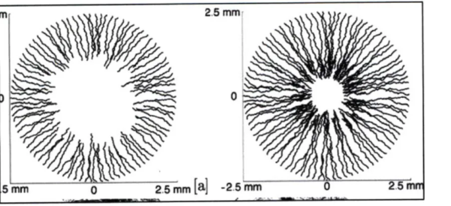
Angiogenesis modeling is a useful tool for understanding the interplay between all the factors that affect it and for the design of experiments of a predictive nature. Over the years various models spanning different scales and focusing on different aspects of angiogenesis have been developed. These can be classified as continuum models (Anderson and Chaplain, 1998; Chaplain et al., 2004; Chaplain et al., 2006; Chaturvedi et al., 2005; Dallon et al., 1997; Levine et al., 2000), and discrete models (Anderson et al., 1998; Chaplain et al., 2006; Stokes et al.,
1991; Mantzaris et al., 2004). Some of the model results are shown in figure 2.
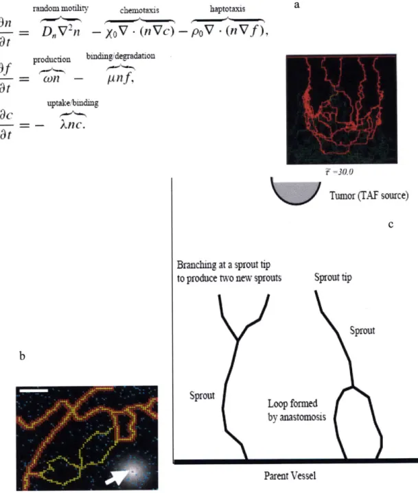
The continuum models are based on conservation equations for chemotactic and haptotactic gradients. In one such continuum model the Chaplain group models a 'tissue response unit', which includes an endothelial cell (EC), tumor angiogenic factor (TAF) and a generic matrix molecule. The numerical solution is obtained from a finite difference approximation subject to no flux boundary conditions and a specified initial condition. They have also developed a
discretized version of the continuum model where the motion of the capillary in response to a tumor is governed by the EC at the tip (Anderson and Chaplain, 1998).
The Cellular Potts Model (CPM) is a lattice-based model developed to describe the behavior of cellular structures and their interactions. It could be an agent-based model, which is a computational model that is based on one (or more) specific component(s) and its effect on the individual cells (agents) being modeled. A 2D agent-based model of angiogenesis based on CPM has been developed by Pierce et al. (2004), where they identify multiple cell types and growth factors. Their cell-level rule-based model of network growth in mesenteric tissue predicts new vessel formation, vessel length extensions and recruitment of contractile perivascular cells in response to localized pressure, circumferential strain and focal application of growth factor. The Sherratt group has used an extension of the Potts model to simulate malignant cells and quantified invasion morphology as a function of cell-cell adhesion (Turner and Sherratt, 2002; Figure 3). In a different approach, the Popel group has developed a multi-scale integrative model with specific modules for various growth factor receptor pairs and ECM proteolysis (Qutub et al., 2009). Their model considers oxygen delivery by hemoglobin-based oxygen carriers (Tsoukias et al., 2007), the cellular response to oxygen in skeletal muscles (Ji et al., 2006) and a cell based model which results in angiogenesis via reorganization of existing capillaries (Qutub and Popel, 2009). Other models include a Random Walk Model (Plank and Sleeman, 2004), which is distinguished by the fact that it places no restrictions on the direction of capillary growth, an individual cell-based 2D mathematical model of tumor angiogenesis in response to a diffusible angiogenic factor (Plank and Sleeman, 2004), and a fractal-based model in which the smaller pieces of the system show 'statistical self similarity' to the whole and the anatomical
entities are given a fractal dimension. Random walk models that incorporate biochemical cascades when VEGF binding occurs have also been developed (Levin et al., 2002). Physiological models, for instance a model of corneal angiogenesis, have also been developed. Jackson and Zheng (2010; figure 4) have developed one such model that integrates a mechanical model of elongation with a biochemical model of cell phenotype variation. Despite the wide variety in modeling approach, most of the models focus on tumor angiogenesis instead of in vitro capillary growth, and may lack one of the following: stochasticity, a 3D framework or simplified binding kinetics, and are therefore difficult to apply in practice for tissue engineering applications. A combination of these characteristics in a model used for tissue engineering applications would be very useful. Finally, model validation in many of the existing models is a challenge due to the difficulty in controlling all important factors in vivo combined with limited capability of most in vitro systems to replicate angiogenesis.
The complex biological processes leading to capillary morphogenesis are a consequence of cell-level decisions that are based on global broadcast signals, limited near-neighbor communication, and stochastic decision-making with feedback control. Integrating these factors, a cell becomes programmed to follow one of several state trajectories that could be characterized as quiescence, division, apoptosis or migration. We have developed a model to address the needs for greater understanding of the process and for a practical tool with predictive capabilities.
iii. Proposed Model Framework
This is a 3D coarse-grained multi-scale hybrid model in which each cell is modeled as an individual decision-making entity and cell-cell interactions are incorporated via the combined
effect of cells on the matrix and the effect of the surrounding matrix in the individual cell decision-making process. Thus, this model demonstrates the phenomenon that when individual cells are modeled independently according to a set of rules and when cell-cell communication is embedded, the cell ensemble results in capillaries with features that can be attained experimentally in bioreactors for controlled tissue engineering purposes. It also provides a platform for bracketing these cell ensemble results into clusters with different sprout characteristics and identifying the factors that affect them. Most importantly, this study presents a model framework designed alongside experimental constraints and one that can simulate capillaries like the ones generated in an in vitro microfluidic system. This model-experiment cross talk is crucial in identifying the effect of individual influential factors on angiogenesis.
A major driving force in this model is its usefulness in predicting the angiogenic response in a closely regulated experimental platform, with the objective of providing validation and of implementing feedback control over a prototypical biological process. One such experimental platform is the microfluidic system recently developed by our group (Vickerman et al., 2008). The first step in analyzing model predictions is to identify a set of relevant sprout characteristics that would be useful in measuring the effect of different conditions and that could be easily measured in real time during an experiment. These features are then compared to the simulation results.
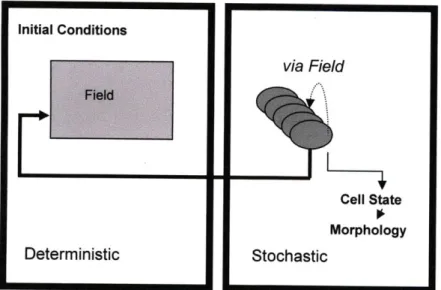
The model is discrete and can be divided into two distinct parts or modules; one is stochastic and the other is deterministic. These modules communicate with each other to predict capillary formation as a function of the local microenvironment, including the effects of growth factors
and matrix properties. This interplay is depicted in Figure 5. This is a 3D lattice model based on Markov processes, where at any time point each lattice point can be occupied by a cell, the matrix or remain empty. A cell can be in one of three states: quiescent, migrating or proliferating. It can also undergo apoptosis, at which point that lattice point becomes empty. Every lattice point that is occupied by matrix is referred to as the 'field' and has associated with it concentrations of the various growth factors and matrix properties. In its current form, the model only includes VEGF, Ang 1 and MMP concentrations and matrix stiffness. However, this can be easily extended to include any number of growth factors and is modular in nature. Capillary features successfully depicted in this 3D model are continuous sprouts, secondary and tertiary branches, and cell clusters - all of which are observed in experiments. 3D modeling enables capillary surface area and protrusion volume calculations in the simulations and their comparison to experiments conducted in microfluidic devices. It also enables the proper representation of the factors in the surrounding matrix and their effects on individual cell responses. The deterministic component of the model includes the diffusion-convection-reaction equations that govern these growth factor concentrations.
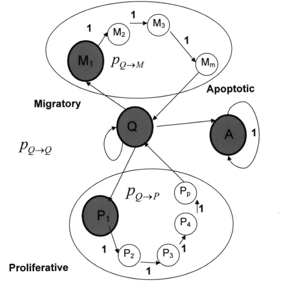
A cell can exist in four main states: Migrating (M), Proliferating (P), Quiescent (Q) and Apoptotic (A). Its transition between states is depicted in Figure 6. Once it undergoes transition to either a migratory or proliferating state, it subsequently passes through a series of sub-states. The number of these sub-states is determined by the time of persistence of migration and the average cell cycle of an individual cell, thereby enabling us to account for differences in the time scales of these processes. Consequently, if a cell can exist in 'm' migratory sub-states and 'p' dividing sub-states, a transition probability matrix is established. Transition probabilities,
e.g.,pe_ , pPQmQ , p_,P( ,PQ-A where M(1) and P(1) are the first steps of the respective processes, depend on the global (g) and local (1) conditions such as growth factor concentration and matrix properties in a manner described below.
The transition of each cell from one state at time t to another at time t+At is stochastic and is a function of its current state, the condition of the surrounding matrix and external governing factors such as the presence or absence of flow, the growth factors present in neighboring matrix and initial matrix stiffness. That is, transition from state X to +At is described as g't =f(t,
U
(g),
U
()), where U (g) are the global or external factors and U (1) are the local factors or the characteristic of the surrounding matrix and measured by the output Y'. Certain variables like growth factor concentrations only affect the local environment while other factors like flow and pressure gradients have a global effect. The difference being, in the case of global influence, the same function is applied at all spatial locations, while in the case of local variables, the changes are calculated at each lattice point. This function is represented in the model as a transition probability.iv. Model Characteristics
a) Assumptions
Some of the basic assumptions underlying the model are:
1. A Hidden Markov Model is applicable to cell decision processes in angiogenesis.
2. Cells can be modeled as independent Markov processes: The cell state at time t+At is independent of its states prior to the one at time t. This is reflective of the assumption that
cell state effects are additive and whatever the cell underwent in prior states has affected its outcome in the penultimate state.
3. A four state transition matrix provides enough information for process evolution: The states used in this model are quiescence, migration, proliferation and apoptosis. It is assumed that these are the most relevant transitions that cells undergo as they form capillaries. Future experiments might support or negate this assumption. It is possible that some other cell state may be important to gain a complete understanding of the process, however, the use of these four states certainly provides enough information to obtain valuable insights.
4. The states of a cell are independent of each other: A cell can either be in migratory or proliferative states. It is also assumed that certain growth factors can independently impact a cell's decision to transition either into proliferation or migration.
b) Stability
The time step (t+At) for the numerical solution of the diffusion equations is equal to 0.1 second in order to preserve stability of the solution as the equations are calculated explicitly. In order to determine the effect of the size of the time step on the accuracy of the numerical solution of the diffusion equations, we decided to run the simulations by reducing At to half the time. After 20 hours, at any given lattice point the concentration of soluble VEGF (Ceg _) differed by less than
c) Sampling Frequency
The sampling frequency of the 'cellular' time step is the frequency with which the cell is allowed to change its step. It should be noted that once a cell decides to go into the migrating or proliferating state, it remains in that state for different lengths of time. It was decided to select a 'cellular' time step of one hour for two primary reasons. A) Initially, this code was designed to make it compatible with time lapse imaging and one hour was the lowest limit of the frequency with which live imaging could be done without dire photo-bleaching effects. B) This is shorter than the time scale of events (migration / cell division) occurring. In order to determine the effect of the size of the 'cellular' time step on the accuracy of the concentrations being calculated, we decided to run the simulations by reducing the time by half. Cells were allowed to make decisions every 30 minutes instead of every hour. When making these comparisons, the number of time steps during which a cell stayed in the migrating / proliferating stage were modified accordingly. At any given lattice point the concentration of soluble VEGF (Cge) differed by
an average of 0.78% near sprouts of similar lengths.
v. Field Equations
The field equations in this model are presented below and can be simplified when required to provide feedback control. The field equations are written in this instance to include one growth factor, VEGF, and one protease, MMP. Similar equations for other factors can be easily incorporated. C,,e e, Cve fb, Cve , Cm, M and M are the concentrations of soluble
VEGF, VEGF bound to matrix, VEGF bound to receptor, MMP, matrix binding sites available for binding to MMP and cleaved matrix, respectively.
The following governing equations describe Cegf, Cvegf , Cb' ,p and M, where Dvee is the
diffusion coefficient of soluble VEGF, D,, is the diffusion coefficient of MMP, and v is the interstitial flow velocity causing convective transport of VEGF. ko ,mand kff ,M are the binding
constants for the reaction between soluble VEGF and binding motifs in the matrix. ko, and
k off are the binding constants for the reaction between soluble VEGF and VEGF receptors on
the endothelial cells.
#
is the density of cells and Cvg ,,, is the number of VEGF receptors perunit volume, equal to the number of receptors on a single cell times
4.
Prv, and Pr, are therate of production of VEGF and MMP by a single cell, respectively.
#
will be set equal to one for those grid points containing a cell (since we assume here a density of one cell per unit volume), and#
= 0 for matrix. kc ,mis the rate at which the matrix is cleaved by MMP.The kinetic reactions for the VEGF, MMP and matrix binding sites (M) are:
Cgf , + Cegf r []C , ,.gr (1)
rate constants- kon _ and k off
<p -+ CM, (2)
production rate- Pr,,
CMM -+ MC, (3)
rate constant- kc ,
The governing conservation equations are those for soluble VEGF:
vegf _S =-4iVC vegf _s+Dvegf V2
Ceg,_+ +R Rs g , (4)
where
Rvegi_ = -k mCves M +kff Cve b
-koncCveg _,Cveg _r + k offc Cvegf r + Prve #
for bound VEGF:
acgb=
R, _b
at
-where
Rvegf _ b rrn vegf _sM -koff Cvegfb
-k CV kc-mCMMP vegf_b for MMP:
aQJm
= -i.VC +D V2C + Rmmpat
MMP MMP wP where Rmm, = PrMMP V (5) (6)and for the concentration of matrix binding sites: m= R (7) at where RM = -k, ,CmmpM
Assuming local chemical equilibrium, and given the fact that VEGF (VEGF-165 Isoform) binding to the matrix (collagen I) at pH 7.4 is negligible (Adrienne et al., 2004), the equations simplify further. Also, there is no convective transport due to interstitial flow, but this can be added to the model easily.
The first two equations are simplified as follows:
"1f -S =D 2
C
+ RDe,
atg s +eg egfs
where
Res =--koncCvgf _Cvegf rec+k off _cCvegf r + Prvee #
and
c
- ~ 0g
at
(9)These equations are discretized and used in instances where all the parameters are known. While most have been experimentally derived, some of the parameter values would still be subject to considerable uncertainty. In those cases, an approximation was made.
The diffusion term in equations (8) is discretized spatially as follows:
(DvegfV 2Cvegf s) x = Dveg *[(Cvegfs)xy,z+,t =yzt - 2 *(Cvegj
s)x,y,z,t +(Cvegs)xyz-,t]/[Z 2]+
Dveg * [(Cvegf s )x+,y,z,t -2 * (Cveg,_s )xyzt + (Cvegf _s )x-,yzt ] / [0 x2] +
Dveg' * [(Cvegs )xy+z,t - 2 *(Cveg s)xyzt +(Cveg s)xy-z,t]/ Y2]
(10)
where Ax, Ay and Az are equal to 10 pm. The diffusion term in
are the spacings of the computational grid in x, y, and z, respectively, and
equation (6) is discretized similarly.
For the reaction terms, the following methodology is used. The concentration of the biomolecules being modeled will locally change in a single time step by an amount that is dictated by local conditions. This change in the concentration is a sum of the local consumption and production of that molecule and expressed as:
(11)
R = AC,,, - AC,c,j and where
ACiCj = (Ci,c )t+, -(Cica )t
ACi,, = (CP,),+At -(C,,j),
These could potentially be experimentally determined by measuring changes in concentration of signaling molecules, MMP and matrix around a single cell. This can be done by using fluorescent collagen and measuring the matrix properties around individual cells. However, as such experimental data for individual cells are not available, these AC values can be empirically established relative to the rates of production and degradation of these substances by quantifying the qualitative effects on individual cells. When those are being ascertained, ACicj and ACjpj represent step functions associated with this change at the
jth
level in the concentration of the ith biomolecule included in the model due to consumption and production by the cells, respectively. In the simulation results included in this study, we have used a two-level change for the biomolecules being considered, i.e. high production/consumption or low production/consumption. These changes depend on the cell state and the surrounding matrix characteristics. One can imagine that instead of having only a high and low value (e.g., wherej = 1 or 2) for each of these reactions, we can have finer increments where each element is dependent on the different permutations and combinations of other factors in the field. The existing model framework allows for such expansion depending on the different pro- and anti-angiogenic factors being considered.The equations are discretized over time and the spatial derivatives are calculated at time t. Equation (8) is discretized as:
A(C t)
2 = ),,,,(12),,,VC +R
where
(Rves )xyz = ACgf _spj - ACvegfs,Ci
and where
ACvegf _sCj = (Cvegf _s,C )t+At - (Cveg _s,cj )
ACvegf sPJ = (Cveg sP ),+ - (Cvei pi)
At a time t, the amount of VEGF produced and consumed via binding to the cells is a function of the cell state and the state of the surrounding matrix concentration of soluble VEGF, i.e. Cvegs
in the lattice. Thus, the reaction terms are evaluated based on the cell state. kn_ and kOffc
values were obtained from literature (Gabhann and Popel, 2007). Hence, the amount of VEGF consumed (ACreg_s,c,,) is determined by the rate equation. However, as it is difficult to obtain
the amount of VEGF produced by an individual cell, it was approximated by the following method. If there is a migrating cell at a given lattice point, we assume it produces a certain amount of VEGF (AC egspl) if the surrounding VEGF concentration is below a certain
threshold and a different amount (ACvegf,,,2) when it is above a threshold. This threshold of the surrounding VEGF is 12 units (or 24 ng/ml normalized to the minimum concentration of VEGF i.e. 2 ng/ml). This was chosen because it has been shown that VEGF induces its own expression
in microvascular endothelial cells in a STAT3-dependent fashion when the cells are treated with 25 ng/ml VEGF (Bartoli et al., 2003).
Assuming negligible interstitial flow, equation (6) is discretized as:
A(Cm)XYZ = D
=D.V2CMO+ (RM), (3
At MMP
The change in MMP concentration due to production in equation (13) was approximated by assuming that the change around a migrating cell (ACmmpp,1) and that around a quiescent or proliferating cell (AZCMMpPp2) are different.
Equation (7) is discretized as:
A(CM) - (RM Y (14)
At
The value of k,, is obtained from literature (Karagiannis and Popel, 2004). The amount of
matrix consumed ACM,c,, is determined by the rate equation and the state of the cell, as a
migrating cell tends to release more MMP that cleaves the matrix.
The field also includes a stabilizing agent i.e. Ang 1. Ang 1 acts on the Tie-2 receptor in endothelial cells and the range of effective activity on Tie-2 receptor has been shown to be 80ng/ml - 800ng/ml [Bogdanovic et al., 2006]. Several reports document robust Tie-2 phosphorylation at greater than 100 ng/ml concentrations [Kim et al., 2000; Papapetropoulos et
al., 2000; Du et al., 2000]. Ang-l inhibits endothelial cell apoptosis through several pathways, which include PI-3 kinase/AKT activation, inhibition of Smac release from the mitochondria, and upregulation of Survivin protein [Harfouche et al., 2002]. Thus, the graded stabilizing effect of Ang 1 is included in the model. This is discretized and included as an effect on cell connectivity and discussed in section vi.
vi. Cell Transitions
The transition probability of a cell from one state to another is dependent on the initial conditions, such as growth factor concentrations in the medium and matrix stiffness. Cell decisions are made once every hour or every 'cellular' time step. Thus, during each hour, a certain number of cells migrate, proliferate, become quiescent and die. These probabilities are empirically derived. We have explored the range of probabilities and identified combinations that depict sprout characteristics seen under certain experimental conditions. The transitional probability to a particular state at time t + 1 can be written as:
PM,t+1 = PQ,t'PQ-+M,t ± PM,1,t ' + PM,m-1,t - PM,m,t
= PQtPQ-M,, + p,, - PM,m,t (15)
PQ,t+1 PQ,t PQ-4Q,t + PM,t + PPp,t - PQ,I PQ-+M - PQ,t PQ--P - PQ-*At (16)
= POt PQPt + p - pp,, (17)
PA,t+1 = PQt *PQAt (18)
where pM , p , p,,, and PA,,+1 are the probabilities that the cell state at time t+1 becomes M,
Q,
P or A respectively.Pg,, PM,t and p, are the probabilities defined as:
PQ,, = p(X, = Q) (19)
PM,, = EP Mi, (20)
i=1 P
PP = p't (21)
and pQ m, pQQ,, PQ.P,t and PQAt are the transition probabilities to migration, quiescence, proliferation and apoptosis, respectively, under the instantaneous global and local conditions. These are expressed as a probability distribution of percentages of transition (equations 22-25). These probabilities are to be experimentally determined. Alternatively, they could be specified functions of the activation of relevant intracellular signaling pathways.
PQ-M,t = PX,.1 = M | X, = Q) (22)
PQ-Q,: =p(X,,, =Q| X, =Q) (23)
p = p(X, = PX =
Q)
(24)vii. Cell Communication
Cell communication is achieved via the cell-cell connectivity factor, MMP release and lateral inhibition.
a. Cell- cell connectivity
Cell- cell connectivity is maintained under two different scenarios:
1. During individual cell migration: as a cell cannot change shape in this model, a temporary or 'temp' cell is used during cell migration to ensure connectivity and remove any bias during lattice evaluation. This ensures that the impact of transition will not affect other cells in the same time step. When a cell migrates from one lattice point to another, its former location is identified as a 'temp' position and for the remainder of that time step the cell occupies both locations.
2. During sprout formation because of cell adhesion and stabilization: to incorporate cell adhesion and stabilization, cell connectivity between two cells is enforced as a field function that is dependent on the states of the two cells being considered and the local field conditions. All cell-cell communication occurs via the field, i.e. the surrounding matrix. Direct cell-cell interactions were avoided to support the independence of each cell. Otherwise, the model would have to deal with joint probabilities of multiple cells, which are quite complex. On the other hand, by making this assumption, we are still ensuring that the essence of cell-cell interactions is included while minimizing model complexity. This is done by a field variable termed the 'connectivity factor'. Anything the cell 'gives' or 'receives' from a nearby cell is done via this field-associated factor.
The local Ang I concentration is directly proportional to the cell connectivity. The probability of a cell to break away and migrate individually is inversely proportional to the connectivity factor.
The connectivity factor is a discrete number that is dependent on cell states and neighboring Ang I concentration. It is classified into three scales: low, medium, high.
The connectivity rules are as follow:
* If a cell is quiescent, the connectivity factor increases by 2, if it is dividing, it increases by 1 and if is migrating, it increases by 3.
" The average Ang 1 concentration, Ang1,rage is defined as
14
Angla,,rage = [Angl], / 14
where i =1... 14 are all the neighboring lattice points
If the average concentration is below 100 ngml, the connectivity factor increases by 1; if it is between 100 ngml1 to 500 ngml-', the connectivity factor increases by 2; and, if the average concentration in greater than 500 ngmlf, it increases by 3.
The connectivity factor has an impact on the time steps the cell tends to stay in the migratory state. Though the default is three time steps, a connectivity factor of 5 or 6 keeps it in that sub-state for a longer time, and a connectivity factor of less that three makes it evaluate its state sooner. It also impacts cell adhesion in the following way. If a cell adjacent to a migrating cell has a relatively low connectivity factor compared to that of its neighbor, it will tend to stay quiescent, resulting in capillary breakage or individual migrating cells.
b. MMP Release:
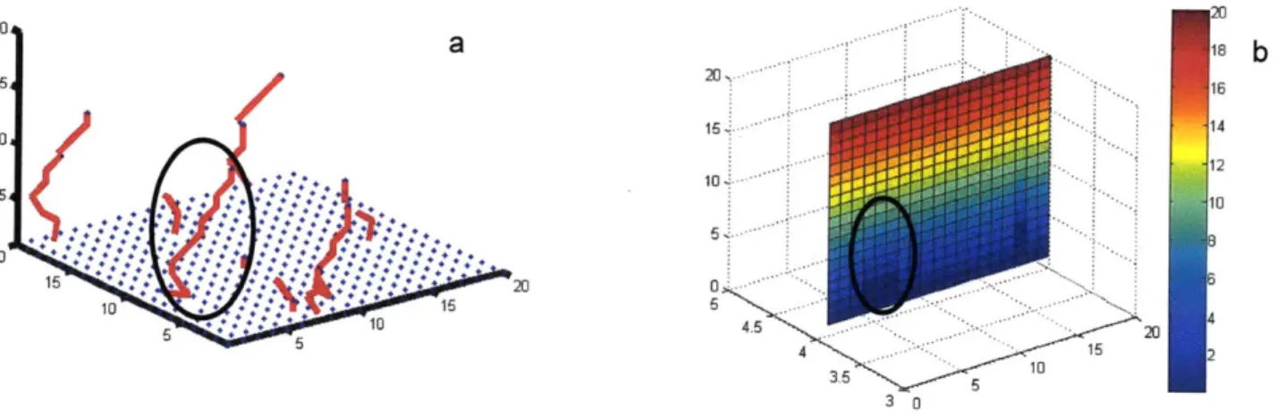
The other tool for cell communication is the release of MMP into the field. The surrounding MMP concentration affects the directionality of migration for neighboring cells. Thus, an individual cell has an impact on its neighbors. It is possible to increase the impact of this tool by involving other molecules released by cells in addition to MMP. Figure 7 demonstrates the effect of migrating cells on the matrix via the MMPs as a change in their concentrations is observed in the region surrounding a developed sprout.
c. Lateral Inhibition:
DL4/ Notch signaling: An important aspect of angiogenesis is lateral inhibition, which is enforced via DL4/ Notch signaling. In order to include this characteristic of the process, cell communication is very important. When a cell at the monolayer is evaluating its state transition, it examines a certain radius of influence. For the current version of the simulation, this has been fixed to a one cell distance. If any of its neighboring cells are in the process of sprout formation, the cell in question has a high probability of staying in the quiescent state.
viii. Rules and Parameters
a) Rules
Certain 'rules' for cell transitions that are incorporated in the mode are outlined below:
1. Initially, a uniform monolayer of cells is assumed to exist on the surface of the matrix. New sprouts are allowed to be initiated for the first four hours. This is implemented to prevent multiple sprout formation and also depicts the biological state when only certain cells in the monolayer sprout and act as 'inhibitors' on nearby cells. This lateral inhibition is enforced via the field.
2. Each cell undergoes a 'decision-making' process, where it can decide to migrate, divide, die or stay quiescent.
3. If a cell has 'decided' to migrate, the direction of migration is stochastic, though it is biased toward the lattice position occupied by matrix that is associated with the highest concentration of chemoattractants and MMP by giving the cell a higher probability to migrate towards that lattice point. It has a lower probability to migrate into any of the other matrix-occupied lattice positions.
4. If a cell has 'decided' to divide, the new cell occupies the matrix-occupied lattice position that is associated with the highest concentration of MMP, as it causes local degradation of the matrix.
5. If a cell dies, its position is occupied by empty space.
6. A cell can migrate only into a lattice position occupied by matrix but can divide into either empty space or matrix.
7. If two cells choose the same lattice point into which to divide or migrate, a tie-breaking rule is applied.
8. A migrating or dividing cell releases MMP into each of the adjacent matrix elements, thus influencing the migration of itself and of neighboring cells. The amount released depends on the state of the cell and can be classified as 'low' or 'high' - the values of which are recorded in Table 1.
9. VEGF is both released and consumed by the cells according to the state of the cell and the surrounding VEGF concentration. As explained earlier and recorded in Table 1, the surrounding local concentration above which VEGF production is 'high' is 12 and that above which VEGF consumption by a cell is 'high' is 10 units.
10. Cells are allowed to divide both at the monolayer and in the stalks.
11. In the current simulations, the number of migration sub-states (m) is three and the number of proliferation sub-states (p) is twenty, where each 'cellular' time step corresponds to approximately one hour.
12. VEGF influences endothelial 'decision-making' via both paracrine and autocrine signaling. Therefore, the deterministic model accounts for the diffusion, consumption and production of VEGF and MMP by the cells.
13. While the sample simulations included in this study account for change in concentration of VEGF and MMP, as well as initial addition of VEGF (40 ngmlfor 20 ngmrl) and/or Ang 1 (500 ngml'1) to the 'field', the module-based algorithm and signaling molecules interacting with the cells in a modular array format ensures that additional molecules can be included easily.
14. In the simulations, the 3D lattice is normalized to the characteristic length of an endothelial cell: ~10 pm. The concentration of the different growth factors and MMP are normalized to the maximum concentration in every simulation.
15. All simulations are recorded 50 hours after the monolayer is established. All
experimental images are documented two days after cell seeding.
b) Parameters
Several parameters have been used in the development of the model. They can be broadly classified into simulation parameters, field parameters and cell parameters.
1. Simulation parameters:
* Grid size: Dependent on the simulation volume. For all model behavior
experiments, the grid size was 20x20x20, and for all experimental matching simulations referred to in chapter 4, the grid size was lOxlOxlO. This is user-specified and can be changed to any size.
* Simulation time: For all simulations this was limited to 48 time steps, implying
48 hours. This is user-specified and can be changed to any length of time.
* Simulation frequency: This is a design specification and was chosen to be one
hour for reasons mentioned in section iii.c (Model Characteristics).
* Location of monolayer: The monolayer was specified at z=1, at one end of the
matrix. This is user-specified.
2. Field Parameters:
The parameters associated with the production and consumption of VEGF and MMP were discussed in section iv (Field Equations) and are recorded in the table 1.
Table 1: The variables used in the four different rate equations described above have two different activities: 'high' and 'low'. These are normalized by the starting concentrations and are therefore dimensionless.
3. Cell Parameters:
e Transition probabilities:
These are parameters that can be varied and be user-specified.
In Model Condition at which In Model
the 'high' values are
High used Low
ACvegf si, ko, C,,g ,C rc + VEGF 0
Change in koff Cveg r concentration > 12
VEGF VEGF due to
consumption
Consumption by a single cell ACvegf sc,2
ACvegfs,P,J 0.05 ± 0.025 VEGF 0.04 0.02
Change in concentration> 10
VEGF VEGF due to
production by a
Production single cell A vegf s,P,2
SCMMP 1 0.6 ± 0.2 Cell is migrating 0.2 0.1
Change in
MMP MMP due to
Production production single cell by a ACMMPP,2
A CMc -Ck,,,CmmpM High release of 0
Change in MMP
Matrix Binding MMP binding sites due to
Q+Q:
This is an input variable that is user-specified. Systematic variations of this parameter have been done and the results are included in section viii (Model Behavior).Q+M: This is an input variable that is user-specified. Systematic variations of this parameter have been done and the results are included in section viii (Model Behavior).
Q-*P: This is an input variable that is user-specified. Systematic variations of this parameter have been done and the results are included in section viii (Model Behavior).
Q+A: This is a fixed variable that could be varied if required. This has been fixed because experiments demonstrated that the growth factors being used did not alter the cell transition to apoptosis. So, this can be fixed at zero and be changed into a cell age dependent factor, or can be changed if a factor that affects cell apoptosis is used.
e Direction transitions:
For migrating: A migrating cell samples all neighboring grid values of MMP and VEGF and identifies the location that has the highest values associated with itself. It then has a 72% probability to move to that location. It has an equal (but comparatively lower; 2%) probability to move to any other lattice point. These values are arbitrary and selected based on the qualitative fact that the cells tend to move towards a higher concentration of chemoattractants and MMP-cleaved matrix.
For dividing: A dividing cell samples all neighboring grid values of MMP and identifies the location that has the higher values associated with itself. It then has a 72% probability to
move to that location. It has an equal (but comparatively lower; 2%) probability to move to any other lattice point. These values are arbitrary and selected based on the qualitative fact that the cells tend to sprout along MMP-cleaved gels and regions with larger pore size.
e Temporal parameters:
Time in migratory state: The default time in migratory state is fixed to be three time steps. This can be changed depending on surrounding Ang 1 concentration, as explained in section vi (Cell Communication).
Time in proliferative state: The default time in proliferative state is fixed to be twenty time steps. This is in congruence with the dividing time of an endothelial cell.
e Others:
Radius of Influence: One cell sphere. This is used to enforce lateral inhibition via DL4/ Notch signaling.
Cell age and apoptosis: There is 5% chance of a cell undergoing apoptosis after 24 hours.
The cell parameters, the transition probabilities will be determined in chapter 4.
ix. Model Behavior
a) Characteristics being measured
Various morphological characteristics can be measured by running the model under different input conditions. In order to exploit the capabilities of the model, we decided to evaluate certain characteristics that could be easily measured in experiments. All simulations were performed in a
20x20x20 grid. The characteristics evaluated were those that most reflect cell population behavior:
1. Average number of sprouts per simulation region 2. Average number of branches per simulation region 3. Average number of anastomoses per simulation region 4. Average length of sprouts
5. Average number of individual migrating cells
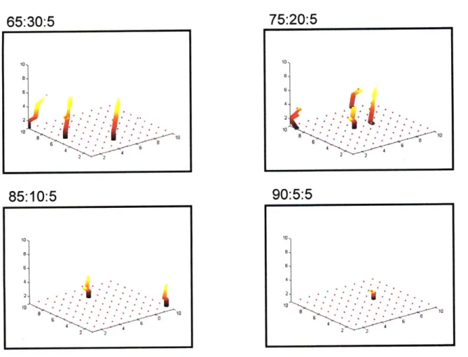
The capillaries in the model can be represented either in the form of individual cells, as shown in figure 1 Od or more commonly as tubular structures, as shown in figure 8. Figure 8 shows the effect of increasing probability of a cell to transition into migration on the number and length of capillaries.
b) Discussion of Results
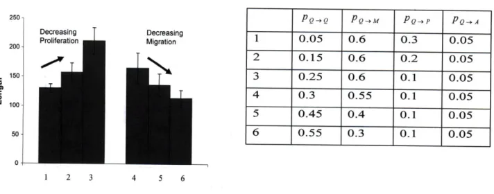
The model can be used to explore how specific features depend on the imposed conditions, as shown in the following examples. Consider first the average protrusion length of cells into the matrix (Figure 9). This is determined by calculating the depth to which cells penetrate at each lattice point in the monolayer in the z direction and assuming unit volume occupied by each cell. Corresponding sets of transitional probabilities are listed in the figure. In the first three transitional sets, the probabilities to migrate and die are held constant, the probability to divide decreases and that to remain quiescent increases. In the next three transitional probabilities sets, the probabilities to divide and die are held constant, the probability to migrate decreases and that to remain quiescent increases. As expected, certain transition probabilities result in higher cell
protrusion into the matrix. As the probability of the cell to remain in the quiescent state increases in the first data set, the protrusion distance increases because of the lower proliferation rate. Thus, fewer sprouts are initiated, and the ones that are formed grow longer. This implies that while proliferation occurs both in the monolayer and in the sprouts, addition of any proliferating agent impacts the proliferation rate in the monolayer more significantly. Hence, the addition of growth factors that stimulate proliferation should result in a larger network of sprouts and/or more cell clusters. In the second data cluster, with higher migration probability, longer sprouts are formed. While the difference in sprout length is not significant with small changes in migration probability, the trends observed are very significant. It provides an insight into the conditions that would give rise to network-like vs. single-sprout-like capillary structures.
1. Continuous Sprouts vs. Cell Clustering
In order to understand the effect of each of the different transition probabilities, the number of different morphologies are recorded when two of the four transitions are kept constant and the other two are systematically varied. Figure 10 shows an average of thirty simulations for each of these conditions.
To determine the effect of increasing specific transitional probabilities, we varied specific ratios (migration (M) to quiescence (Q); proliferation (P) to quiescence (Q); and migration (M) to proliferation (P)) systematically by keeping the other two constant in each case. The results observed for each of the variations mentioned above are depicted in Figures 10 and 11. As the M/Q ratio increases (Figure 10a), the number of individual migrating cells increases and the number of cell clusters at the monolayer decreases. This is because at a certain fixed transition
probability of proliferation, as the tendency of cells to migrate increases, cluster formation decreases. However, discontinuous sprouts or clusters formed away from the monolayer show a bimodal response. At the first peak, these clusters tend to be broader, and at the second peak (when the tendency to migrate is higher than that to proliferate), these clusters tend to be longer. This behavior is clearly seen when capillaries are plotted as an aggregate of individual cells and not tubular structures as shown in all other simulation representations. Figure 10d shows the distinction between the optima for discontinuous sprouts clearly. At lower M/Q ratios, these clusters tend to aggregate more than at higher ratios. When the ratio of migration to quiescence nears one, the number of such 'floating clusters' decreases. This is also the condition that causes an increase in the number of continuous cell sprouts. This shows that these two morphologies lie in two distinct areas in the space map of the different transition probabilities.
A crucial element in capillary morphology prediction is identifying the balance between the transition probabilities of migration and proliferation. Figure 10b shows the effect of varying these two transition probabilities, keeping the transition to quiescence and transition to apoptosis rates fixed at 15% and 5%, respectively. The most relevant prediction is that the number of continuous probabilities peak when this ratio nears one. Though the number of cell clusters in the matrix does not change much, these clusters, like the clusters at the monolayer, tend to become larger as this ratio increases.
The simulations in Figure 10c were generated while keeping the transition probability of migration fixed at 15% and the transition probability of apoptosis fixed at 5%. While the number of continuous sprouts and discontinuous sprouts or cell clusters in the matrix remains unchanged
as the ratio increases, it is also important to note that at this fixed transition rate for migration, very few continuous sprouts are formed. Since this lies in the first half of the curve that determines the effect of migration on sprout formation as shown in Figure 10a, it is verified that sprout formation is optimal at a higher migration transition probability. The number of single migrating cells decreases and the number of clusters at the monolayer increases as the P/Q ratio increases.
The customary capillary morphology found in vivo is continuous sprouts, and its ratio to each of the other morphologies as a function of the ratio of the transition probabilities between migration and quiescence, proliferation and migration, and proliferation and quiescence are shown in Figure 11. As expected, the curves peak when there is a balance between migration and quiescence, which translates into effective capillary induction and stabilization (Figure 11 a). The model predicts that the ratio between proliferation and quiescence should be increased in order to increase the number of continuous sprouts in comparison to individual migrating cells (Figure 11 c). Again, as expected after observing Figure lOb, the number of continuous sprouts is maximized in comparison to any other capillary morphology when the ratio of transition proliferation to that of transition : migration tends towards one (Figure 11 b).
Figures 12, 13 and 14 are contour graphs that plot the change in M/Q ratio on the y axis and the change in P/Q ratio on the x axis. They help identify the 2D space where there is maximum likelihood of obtaining a higher number of continuous sprouts (Figure 12), discontinuous sprouts / cell clusters (Figure 13) and cell clusters at the monolayer (Figure 14). It is observed that the peak of the continuous sprouts contour graph lies in one of the troughs of the discontinuous