Bucket Elimination Algorithm for Dynamic Controllability Checking of Simple Temporal Networks with Uncertainty
Texte intégral
Figure
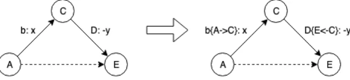
![Figure 6: Triangulation rules carried over from the symmet- symmet-ric reduction rules in [Morris2006]](https://thumb-eu.123doks.com/thumbv2/123doknet/14186553.477242/4.918.119.401.92.366/figure-triangulation-rules-carried-symmet-symmet-reduction-morris.webp)

Documents relatifs
Later Pumplfn ([3], [4]) introduced the category PC of positively convex spaces and the category SC of superconvex spaces.. the categories obtained by.. reqtriction
Given a Hilbert space H characterise those pairs of bounded normal operators A and B on H such the operator AB is normal as well.. If H is finite dimensional this problem was solved
We also perform a cluster analysis, which reveals that, in all three networks, one can distinguish two types of nodes exhibiting different behaviors: a very small group of active
Given that order and direction cannot be equally fundamental, we have to choose: I say that order is the more fundamental characteristic, and that the appearance of direction is
On the other hand, it was showed in [MY] that generic pairs of regular Cantor sets in the C 2 (or C 1+α ) topology whose sum of Hausdorff dimensions is larger than 1 have
In this paper, we construct a graph G having no two cycles with the same length which leads to the following
C7 – REMOTE SENSING & PHOTOGRAMMETRY March 2019 Although programmable calculators may be used, candidates must show all formulae used, the substitution of values
Mean reaction times (RT) in milliseconds (ms) of different versions of the sentences (a = mixed Romani-Turkish, b = all Turkish, c = Romani with Turkish codeswitching, d = Romani
