Publisher’s version / Version de l'éditeur:
Building and Environment, 36, May 4, pp. 407-419, 2001-05-01
READ THESE TERMS AND CONDITIONS CAREFULLY BEFORE USING THIS WEBSITE.
https://nrc-publications.canada.ca/eng/copyright
Vous avez des questions? Nous pouvons vous aider. Pour communiquer directement avec un auteur, consultez la
première page de la revue dans laquelle son article a été publié afin de trouver ses coordonnées. Si vous n’arrivez pas à les repérer, communiquez avec nous à [email protected].
Questions? Contact the NRC Publications Archive team at
[email protected]. If you wish to email the authors directly, please see the first page of the publication for their contact information.
NRC Publications Archive
Archives des publications du CNRC
This publication could be one of several versions: author’s original, accepted manuscript or the publisher’s version. / La version de cette publication peut être l’une des suivantes : la version prépublication de l’auteur, la version acceptée du manuscrit ou la version de l’éditeur.
For the publisher’s version, please access the DOI link below./ Pour consulter la version de l’éditeur, utilisez le lien DOI ci-dessous.
https://doi.org/10.1016/S0360-1323(00)00022-6
Access and use of this website and the material on it are subject to the Terms and Conditions set forth at
Three-dimensional analysis of thermal resistance of exterior basement insulation systems (EIBS)
Maref, W.; Swinton, M. C.; Kumaran, M. K.; Bomberg, M. T.
https://publications-cnrc.canada.ca/fra/droits
L’accès à ce site Web et l’utilisation de son contenu sont assujettis aux conditions présentées dans le site LISEZ CES CONDITIONS ATTENTIVEMENT AVANT D’UTILISER CE SITE WEB.
NRC Publications Record / Notice d'Archives des publications de CNRC: https://nrc-publications.canada.ca/eng/view/object/?id=d113f5ec-1fc4-420b-8580-132bb6b9684c https://publications-cnrc.canada.ca/fra/voir/objet/?id=d113f5ec-1fc4-420b-8580-132bb6b9684c
Three-dimensional analysis of thermal
resistance of exterior basement insulation
systems (EIBS)
Maref, W.; Swinton, M.C.; Kumaran, M.K.;
Bomberg, M.T.
A version of this paper is published in / Une version de ce document se trouve dans : Building and Environment, v. 36, no. 4, May 2001, pp. 407-419
.
www.nrc.ca/irc/ircpubs
NRCC-43090
3-D ANALYSIS OF THERMAL RESISTANCE OF EXTERIOR BASEMENT INSULATION SYSTEMS (EIBS)
W. Maref 1, M.C. Swinton 1, M.K. Kumaran 1 and M.T. Bomberg 1
(1) National Research Council of Canada
Institute of Research in Construction, M-24 Montreal Road, Ottawa K1A 0R6
Wahid Maref Research Associate Tel. 1 (613) 993 5709 Fax. 1 (613) 954 3733 E-mail: [email protected] Mike Swinton
Senior Research Officer Tel. 1 (613) 993 9708 Fax. 1 (613) 954 3733 E-mail: [email protected]
Kumar Kumaran
Senior Research Officer Tel. 1 (613) 993 9611 Fax. 1 (613) 954 3733 E-mail: [email protected]
Mark Bomberg
Senior Research Officer Tel. 1 (613) 993 3662 Fax. 1 (613) 954 3733 E-mail: [email protected]
Keywords Exterior insulation, thermal resistance, thermal performance, heat transfer,
basement walls, 3-D model, calculation, analysis, temperature, heat flow, heat loss.
Abstract
A consortium1 research project was initiated to determine the field performance of various thermal insulation products as applied in the exterior insulation basement system (EIBS). Initially a two-dimensional analytical tool was used to derive the thermal
transmission characteristics from an array of temperature measurements performed over a period of two years. Results immediately showed the influence of lateral heat flux
between various products that differed in thermal transmission properties. Therefore, development of a three dimensional model became imperative.
This paper gives the theoretical and numerical approaches adopted to develop a three-dimensional computer model of heat transfer. The implicit Spline Method was selected for the problem solver. The applicability of the model was verified using measured data on temperature distributions at several material interfaces. Then the model was used to estimate the effect of lateral heat flows.
The paper also briefly reports the experimental details and presents results on model verification.
1
The consortium included Expanded Polystyrene Association of Canada, Canadian Urethane Foam Contractors Association, Owens Corning Inc. and Roxul Inc.
Nomenclature
C Specific heat [ J/kg.K]
i
K Thermal conductivity in x direction [ W/m.K]
j
K Thermal conductivity in y direction [ W/m.K]
k
K Thermal conductivity in z direction [ W/m.K]
Q Heat generation [W/m3] t Time [s]
Subscripts
i Nodal point value j Nodal point value
ρ Density [kg/m³] T0 Initial temperature[oC]
S1, S2 and S3 Boundary surfaces
t ∆ Time step [s] z and y x ∆ ∆
∆ , , Step of spatial discretisation
in x, y and z direction [m]
k Nodal point value s On boundary surface
BACKGROUND
Over the recent decades, a large part of basements in newly built Canadian houses became used as a habitable space. This, combined with increased requirements for energy conservation, resulted in the development of many insulated basement systems. While thermal insulation may be placed either on the inside or on the outside of the basement wall, the material choice and the insulation placement may affect overall performance of the basement wall. Some external insulation systems, in addition to controlling heat losses, may also increase durability of the basement wall.
In this context, the Canadian thermal insulation industry, working together with the National Research Council, decided to revisit2 the design and performance of external insulation basement systems (EIBS). Over the two-year period from June 1996 to June 1998, ten expanded polystyrene (EPS), two spray polyurethane foam (SPF), two mineral fibre insulation (MFI) and two glass fibre insulation (GFI) specimens were placed on the exterior of the basement wall in an experimental building located on NRC Campus in Ottawa.
This research project involved a number of material and system issues. Material considerations involved selection of existing and new thermal insulation products (being under development). These products were placed side-by-side on the basement wall to create virtual test compartments. The system considerations involved two different technical solutions to protect the above-grade part of the EIBS. Furthermore, different
2
conditions for surface water drainage were implemented on East and West walls of the NRC experimental basement facility.3
Because of the wide scope of the basement research, this project is reported in four parts: 1. Development of analytical tools to increase confidence in the experimental
results and facilitate the analysis of the field data
2. Reporting and analyzing results obtained from the experimental basement 3. Placing the thermal and moisture performance of expanded polystyrene in
below-grade application in context of other research (state-of-the-art review to identity future research needs on the material side)
4. Reporting and analyzing the system effects in context of other research (state-of-the-art review to identity future research needs for development of basement systems)
The first part of the EIBS project is addressed in this paper, which presents theoretical and numerical aspects of 3-D computer model developed as a part of integrated approach (modelling and testing). The capabilities of this model to enhance the analysis of experimental results will be demonstrated in the next paper (Swinton et al) [3].
1. EXPERIMENTAL APPROACH
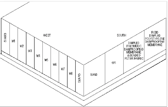
To evaluate performance of exterior basement insulation, different materials were installed on the exterior surface of concrete basement walls. As shown in Figure 1, eight test specimens were placed side-by-side, on each of two basement walls (east and west) insulating a whole wall with approximately 76-mm thick and 2.4 m high specimens. On the interior of the wall, a 25-mm layer of expanded polystyrene (EPS) board was installed
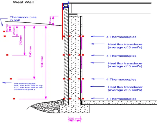
over the entire surface. At 3 vertical locations on each test wall, cut-outs were made and calibrated EPS specimens, with identical thickness, were tightly inserted. These specimens were used for determination of transient heat flux entering the wall (Bomberg et al) [4].
Thermocouples were placed at the boundary surfaces as well as the interfaces of each layer in the wall, in an array consisting of 16 points per tested compartment. All sensors placed on the west wall are shown in Figure 2.
The parameters monitored in the EIBS are:
1. Surface temperatures, on both sides of the calibrated specimen, the concrete and the test specimens
2. Heat flux across the calibrated insulation specimens
3. Soil temperatures from 1 to 2 m away from the specimens, and at 5 depths 4. Interior basement air temperature (average of 4 readings)
5. Exterior air temperature (at north face, shielded from sun)
6. Relative humidity (RH) and other parameters of indoor and outdoor environments.
The instrumentation package consisted of approximately 145 thermocouples, 2 humidity sensors, 21 calibrated insulation specimens (heat flux transducers), 4 junction boxes, and a data acquisition unit operated by a computer.
1.1 Data acquisition
The collection of data was done with an automated data acquisition and scanning system, and a high precision multi-meter to measure separate thermocouples, serial thermopiles
and relative humidity sensors. All thermocouples and power signals were routed through a HP command module (HP E1406) connected to a PC 486/50. Measurements were taken every 2 minutes and averaged by the software package (HP_VEE) for 10-minute intervals for the wall thermocouples (5 readings), and 30-minute intervals for the soil thermocouples (15 readings).
1.2 Duration of the experimental program
The data acquisition system was commissioned in the spring of 1996 and monitoring started after adjusting the air conditioning system on June 5, 1996. The monitoring ended on June 5, 1998, exactly 2 fully years of monitoring.
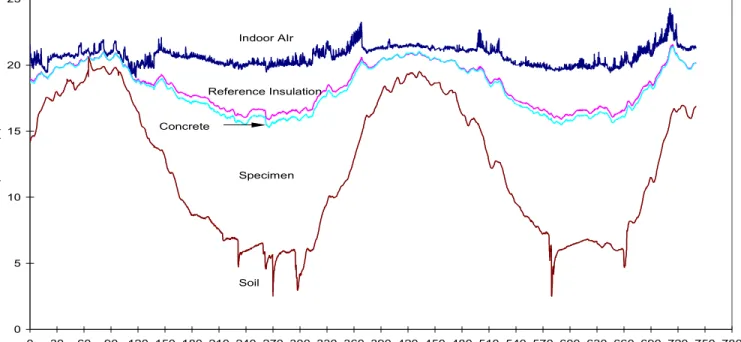
Figure 3 shows measured temperatures of indoor air, calibrated insulation specimens, concrete, and soil surface in the “mid-position” of the wall over a period of two years. The spikes in the interface between soil and the EIBS correspond to thaw periods with a heavy rainfall. Observe that these effects do not appear to affect the temperature on the concrete surface, i.e., behind the external insulation.
1.3. Preliminary results
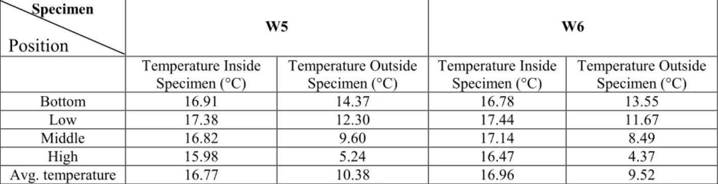
Examination of preliminary results highlighted difficulties in establishing the precision of thermal testing without addressing 3-D effects. This is best illustrated by comparing W5 and W6 tested wall sections.
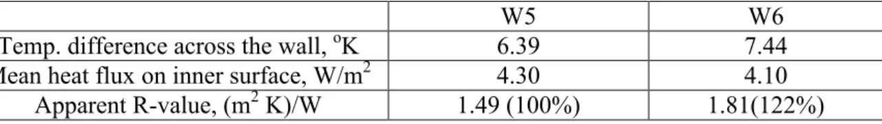
Table 1 shows average temperature difference across the insulation layer and heat fluxes entering each of these two tested wall sections. These results are averaged over a period of one week to approximate the steady state and use the ratio between the temperature
difference and the heat flux as an indicator of thermal resistance. When thermal resistance of W5 is taken as a benchmark (100%), the ratio between W6 and W5 specimens is 122%. This result is, however, much lower than the ratio of 164 percent obtained from the initial, laboratory measurements of thermal resistance performed on specimens W5 and W6. Even if the R-value of W6 specimen was corrected for the effect of foam ageing, the difference between one-dimensional estimate and the measured results is significant. This difference highlights the need for 3-D model application.
1.5. Discussion
As the test set-up involved diverse thermal insulating materials placed next to each other, the presence of lateral heat flow was inevitable. In the case of specimen W6 (closed-cell, gas-filled thermal insulating foam), some heat would be conducted laterally through the concrete wall and pass through the adjacent specimen, which has a lower thermal resistance. The lateral heat flow may explain that the ratio of estimated thermal resistance of two adjacent specimens W5 and W6, shown in Table 1, is smaller than the ratio indicated by the laboratory comparison.
To evaluate effects of lateral heat flow on the precision of the field measurements, a new task was added to the EIBS project, namely development of a 3-D model. The first question was then, how to discretise the continuous equations to arrive at the system, which is easy to solve with numerical techniques.
2 SOLUTION OF THE DIFFERENTIAL EQUATION OF HEAT CONDUCTION 2.1 State of the art of analytical techniques
Several different techniques of numerical analysis for solving transient heat conduction problems, such as the finite-difference, finite-element, and boundary integral equation methods have been presented in the technical literature.
Bhattacharya [5] and Lick [6] applied the improved finite-difference method (FDM) to time-dependent heat conduction problems with step-by step computation in the time domain. The finite-element method (FEM) based on variational principle, was used by Gurtin [7] to analyze the unsteady problem of heat transfer. Emery and Carson [8] as well as Visser [9] applied variational formulations in their finite-element solutions of nonstationary temperature distribution problems. Bruch and Zyvoloski [10] solved the transient linear and non-linear two-dimensional heat conduction problems using the finite-element weighted residual process. Rources and Alarcon [11] presented a formulation for a two-dimensional isotropic continuous solid using the boundary integral equation method (BIEM) with a finite-difference approach in the time domain. Combined application of BIEM and the Laplace transform to transient heat conduction problems started in 1970 with a paper by Rizzo and Shippy [12]. Later, Liggett and Liu [13] and Cheng and Liggett [14] applied this scheme to the linear time-dependent problems. Chen et al [15] successfully applied a hybrid method based on the Laplace transform and the FDM to transient heat conduction problems.
The disadvantages of these methods are the complicated procedure, need for large storage and long computation time. Wang et al [16] used the implicit spline method of splitting to solve the two and three-dimensional transient heat conduction problems. The method is applied to homogeneous and isotropic solid.
A cubic spline method has been developped in the numerical integration of partial differential equations since the pioneering work of Rubin and Graves [17], and Rubin and Khosla [18]. This method provides a simple procedure, small storage, short computation time, and a high order of accuracy. Furthermore, the spline method has a direct representation of gradient boundary condition.
In this paper, an implicit spline method is used for solution of three-dimensional transient heat conduction problems for a non-homogeneous medium. This method, for each computation step, treats the problem as a one-dimensional case in the implicit form and only one tridiagonal system is evaluated. In section 2, a spline scheme of splitting is presented. In section 3, the stability of the method is assessed.
2.2 Mathematical formulation
The governing differential equation for transient heat conduction in a homogeneous and isotropic solid is given by:
Q z T K z y T K y x T K x t T C i j k ÷÷+ ø ö ç ç è æ ÷÷ ø ö çç è æ ∂ ∂ ∂ ∂ + ÷÷ ø ö çç è æ ∂ ∂ ∂ ∂ + ÷÷ ø ö çç è æ ∂ ∂ ∂ ∂ = ∂ ∂ ρ (2.1)
This equation, with suitable boundary and initial conditions, represents the problem of temperature distribution at any time and at any point of the volume, under consideration.
Different density ρ but constants for each type were used. They were determined as the average of several specimens. Discussion on EPS variability in physical properties and the method that has been used for their homogenisation is currently published [19]. The specific heat C which is appears in the eqs.(2.1) and consistently further was from the Handbook of Heat Transfer.
The above quoted paper [19] deals with thermal conductivity coefficient as it varies with material thickness, temperature, density of specimen and specific mass extinction coefficient. As far as Q is concerned, it is a result of gradient T and K.
Thermal conductivity Ki in eqs.(2.1) does not include any effect of latent heat transfer
that may be induced by the humidity changes. 2.2.1 Special treatment at the interface
Assuming the perfect contact, i.e., when heat fluxes φicand φci are equal, the following
equation is obtained:
(
)
c i i i c i i c c i i i i X K X K X X K K K , 1 1 , 1 , , 1 2 / 1 + + + + + + + =and the interface temperature is given by:
c i i i c i i c i i i i c i c X K X K T X K T X K T , 1 1 , 1 , 1 1 , + + + + + + + =
2.2.2 Boundary and initial conditions
The temperatures are imposed at the surfaces.
1 1 on surface S T T = S 2 2 on surface S T T = S
3
3 on surface S
T
T = S
and the initial condition is ) , , ( ) 0 , , , (x y z T0 x y z T =
where the union of the surfaces S , 1 S and 2 S forms the complete boundary of the solid 3 of volume V; S , 1 S and 2 S are part of boundary on which the temperatures T are 3 prescribed.
2.2.3 Implicit Spline Schemes
The implicit spline schemes of splitting for the numerical solution of equation (2.1) are (Wang) [20] ÷ ø ö ç è æ + ∆ + = + + P Q C t T T n k j i n k j i n k j i 3 1 1 . 1/3 3 / 1 ρ (2.2a) ÷ ø ö ç è æ + ∆ + = + + + Q R C t T Tinjk injk injk 3 1 1 . 2/3 3 / 1 3 / 2 ρ (2.2b) ÷ ø ö ç è æ + ∆ + = + + + Q S C t T Tinjk injk injk 3 1 1 . 1 3 / 2 1 ρ (2.2c) where k j i
T , Pijk, Rijk, Sijk are the spline approximation of
( )
T ijk,k j i i x T K x ÷ ÷ ø ö ç ç è æ ÷÷ ø ö çç è æ ∂ ∂ ∂ ∂ , k j i j y T K y ÷ ÷ ø ö ç ç è æ ÷÷ ø ö çç è æ ∂ ∂ ∂ ∂ , k j i k z T K z ÷ ÷ ø ö ç ç è æ ÷÷ ø ö çç è æ ∂ ∂ ∂ ∂
(
)
(
)
(
)
) 3 . 2 ( . 6 3 . 6 , , 1 2 / 1 , 1 , 1 2 / 1 , 1 , 1 , , 1 , 1 a x T T K x T T K P x P x x P x k j i k j i k j i i k j i k j i k j i i k j i k j i k j i k j i k j i k j i k j i ∆ − − ∆ − = ∆ + ∆ + ∆ + ∆ − − + + + + + + −(
)
(
)
(
)
) 3 . 2 ( . 6 3 . 6 , , 1 , 2 / 1 , 1 , , 1 , 2 / 1 , 1 , , 1 , 1 , , 1 , , 1 , b y T T K y T T K R y R y y R y k j i k j i k j i j k j i k j i k j i j k j i k j k j i k j i k j i k j i k j i ∆ − − ∆ − = ∆ + ∆ + ∆ + ∆ − − + + + + + + −(
)
(
)
(
)
) 3 . 2 ( . 6 3 . 6 , 1 , 2 / 1 1 , 1 , 2 / 1 1 , 1 , , 1 , 1 , , c z T T K z T T K S z S z z S z k j i k j i k j i k k j i k j i k j i k k j i k j i k j i k j i k j i k j i k j i ∆ − − ∆ − = ∆ + ∆ + ∆ + ∆ − − + + + + + + − where 0 , 1 > − = ∆xijk xijk xi− jk , 0 , 1 , > − = ∆yijk yijk yi j− k , 0 1 , > − = ∆zijk zijk zij k−If boundary conditions are given, we obtain spline solutions of equation (2.1) from equations (2.2) and (2.3).
The equation (2.2a) can be written in the following form
3 / 1 3 / 1 + + = + n k j i k j i k j i n k j i E F P T (2.4)
From Equation(2.2a) and (2.4), we find
1 , 2 , 3 / 1 , 1 3 / 1 3 / 1 , 1 + + = = − + + + + − BT CT D i N T A n i k j i i n k j i i n k j i i (2.5) where k j i i k j i k j i i x K F x A ∆ − ∆ = − − 2 / 1 , 1 6 k j i i k j i i k j i k j i k j i i x K x K F x x B , 1 2 / 1 2 / 1 , 1 3 + + − + ∆ + ∆ + ∆ + ∆ =
k j i i k j i k j i i x K F x C , 1 2 / 1 , 1 , 1 6 + + + + ∆ − ∆ =
(
)
k j i k j i k j i k j i k j i k j i k j i k j i k j i k j i i F E x F E x x F E x D , 1 , 1 , 1 , 1 , 1 , 1 6 3 6 + + + + − − ∆ + ∆ + ∆ + ∆ =Under proper conditions this system can be solved with Thomas Algorithm (A.D.I Method) [21].
The same techniques are used for solving equations (2.2b) and (2.2c) for determining
3 / 2 + n k j i T and Tinj+k1.
2.2.4 Truncation error and stability
The spatial accuracy of the spline approximation for interior points has been considered in the work of Rubin and Khosla [18].
For diffusion terms, cubic spline approximation has second-order accuracy, which can be maintained even with rather large nonuniformities in mesh width.
For the linear heat conduction equation (2.1) with Q=0, the interior point stability of scheme (2.2) can be assessed with the Von Neumann Fourier decomposition for
t cons h z y xijk =∆ ijk =∆ ijk = = tan ∆ . Let (kih k jh kkh) I k k k e T Tinjk n 1/3 1 2 3 3 2 1 3 / 1 . + + + + = , (kih k jh kkh) I k k k e T Tinjk n 2/3 1 2 3 3 2 1 3 / 2 . + + + + = (kih k jh k kh) I k k k e T Tinjk n 1 1 2 3 3 2 1 1 . + + + + =
( )
÷ ø ö ç è æ + + ± + + ± =Tkk k eI k i h k jh kkh Tn n k j i 3 2 1 3 / 1 3 2 1 3 / 1 , 1 1 .(
)
÷ ø ö ç è æ + + ± + ± + =Tkkk eI kih k j h k kh Tn n k j i 3 2 1 3 / 2 3 2 1 3 / 2 , 1 , 1 .(
)
÷ ø ö ç è æ + + ± ± + + =Tkkk eI kih k jh k k h Tinjk n 1 1 2 3 1 3 2 1 1 1 , . Let Direction x in Factor ion Amplificat T T n n k k k k k k 3 2 1 3 / 1 3 2 1 1 + = ξ Direction y in Factor ion Amplificat T T n n k k k k k k 3 / 1 3 2 1 3 / 2 3 2 1 2 + + = ξ Direction z in Factor ion Amplificat T T n n k k k k k k 3 / 2 3 2 1 1 3 2 1 3 + + = ξ 1 , 2 3 2 1 1 3 2 1 =− = + I Factor ion Amplificat Global T T n n k k k k k k ξFrom equation (2.2a) and (2.3a), we find
( ) ( )
(
)
(
)
h k e eI k h i I k h i 1 2 / 1 2 / 1 1 cos 2 1 3 1 1 1 1 + + − + = − − + α α α ξ where(
)
0 . . 2 2 / 1 2 / 1 + > ∆ = + − h C K K t i i ρ α 2 / 1 2 / 1 2 / 1 2 / 1 − + + + + = i i i i K K K α2 / 1 2 / 1 2 / 1 2 / 1 − + − − + = i i i i K K K α
In some manner ξ and 2 ξ are calculated. 3
( ) ( )
(
)
(
)
h k e eI k h j I k h j 2 2 / 1 2 / 1 2 cos 2 1 3 1 1 2 2 + + − + = − − + β β α ξ ( ) ( )(
)
(
)
h k e eI k h k I k h k 3 2 / 1 2 / 1 3 cos 2 1 3 1 1 3 3 + + − + = − − + γ γ α ξ Where(
)
0 . . 2 2 / 1 2 / 1 > + ∆ = + − h C K K t j j ρ β and(
)
0 . . 2 2 / 1 2 / 1 + > ∆ = + − h C K K t k k ρ γ From ξ =ξ1.ξ2.ξ3 we have ξ ≤ξ1.ξ2.ξ3ψ has to be bounded when t tends to 0, then ξ have to be lower or equal to 1.
The Von Neuman’s condition for this scheme necessary for the suppression of all error growth requires that the spectral radius ξ ≤1.
With each of the coefficients, ξ1 ξ2 ξ3 less than 1 , their product is less than 1 and the scheme (2.2) is unconditionally stable with arbitrary values of ∆t,h,Ki,Kj andKk.
2.3 Computational algorithm
The heat transfer through the basement wall does not involve heat generation. By using the equation (2.5), one can create the following system of linear equations:
Where A is an (N x N) matrix and T and B are (N) vectors. The subscript of A, T and B range from 1 to N as follows:
ú ú ú ú ú ú ú ú ú ú ú ú ú û ù ê ê ê ê ê ê ê ê ê ê ê ê ê ë é = − − − − − − n n n n n n n n n n a a a a a a a a a a A , 1 , , 1 1 , 1 2 , 1 3 , 2 2 , 2 1 , 2 2 , 1 1 , 1 . . . . . . ÷ ÷ ÷ ÷ ÷ ÷ ÷ ÷ ÷ ø ö ç ç ç ç ç ç ç ç ç è æ = n T T T . . . . . 1 , ÷÷ ÷ ÷ ÷ ÷ ÷ ÷ ÷ ÷ ø ö çç ç ç ç ç ç ç ç ç è æ − − = + − 1 1 2 0 1 1 . . . n n n n T C D D D T A D B Where: ï ï î ï ï í ì = + = = = = = = + else a i j for C a i j for B a i j for A a j i i j i i j i i j i 0 1 , , , , 1
The above system consists of a tridiagonal system of linear equations. To solve this system of equations, the Thomas algorithm is used [22].
3 RESULTS AND DISCUSSIONS
While the complete review of results from the Basement Consortium Research project is presented elsewhere (Swinton et al.) [3], the current paper elucidates and quantifies the effect of lateral heat flow with the help of the 3-D model.
3.1 Benchmarking of the model
This 3-D model is benchmarked with spatial and temporal temperature distributions. In the initial calculations, one forces the model to agree with the measured conditions by varying thermal conductivity of the material until finding the best fit. However, there are hundreds of subsequent calculations in which no further adjustment of material properties is allowed and where the model is used in a standard, predictive manner.
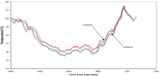
Figure 5 shows temperatures on both sides of the exterior insulation (soil and concrete). The results of 3-D calculations on the test wall W6 during the second year are compared with the measured values. The acceptable agreement between measured and calculated temperature fields permits application of the model to quantify the effect of lateral heat flow.
3.2 Application of the model
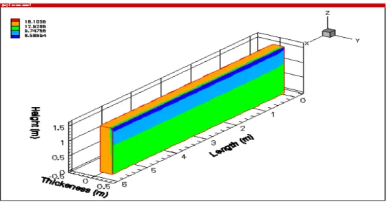
As shown in Figure 6, a reference calculation eliminating the lateral heat flow was called a 2-D solution. In this case, the model calculations were performed assuming that all
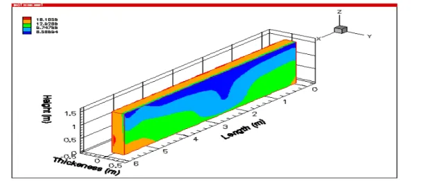
materials properties are identical to that of EPS placed in W5 position (i.e., material on the side of the tested specimen). As shown in Figure 6, except for area adjacent to the corners, temperature is uniformly distributed along the depth of the basement wall. In contrast to that uniformity, Figure 7 shows the distribution of temperature on the surface of the insulation, calculated for the actual temperature field which was measured by termocouples on the boundary of the control volume.
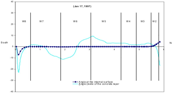
The model calculations, as previously discussed, were performed at three different positions where heat flux incoming into the concrete wall was continually measured. Within these three locations the top position of the wall was the most sensitive to lateral heat flow. Figure 8 shows the angle of heat flux vector relative to normal direction at the top position. It is evident that thermal insulating system tested at the W6 position has higher resistance to the heat flow than the adjacent materials W5 and W7. Moving from the centre towards the adjacent test specimen, one may observe that lines of heat flow start to deviate from the normal direction, reaching a maximum angle of about 10 degrees. Lack of the symmetry in Figure 8 implies that the thermal resistance of EIBS in W5 differs from that in W7 location. Also the performance of corner guards W8 and W2 is different, though Figure 8 shows that the width of these guards appear adequate to eliminate major disturbances from the adjacent test areas (W7 and W3).
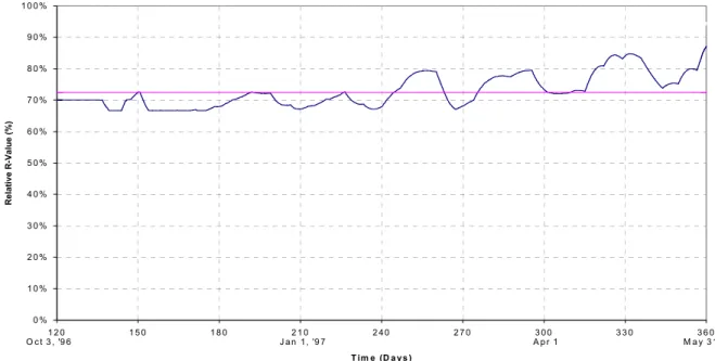
Finally, Figures 9a, 9b, 10a and 10b show the average relative thermal resistance of the specimen W6 when applying different models to the measured data (temperatures and heat fluxes) in the control volume during the first and second year of testing.
The benchmark (100 percent) is the laboratory determined, initial value of thermal resistance of the specimen. The arbitrary nature of this benchmark will be discussed when discussing part 3 of this research project, nevertheless it is sufficient for comparative purposes. Figures 9a, 9b, 10a and 10b show such a comparison. Figure 9a and 9b show results obtained with the 3-D analysis during the first year and the second year of testing, while Figure 10a and 10b show the same calculations when the lateral heat flow component is eliminated (2-D model). These calculations are performed for the period during the second year of testing in which one-directional heat flow is prevailing (days 510 to 660).
Figures 9a, 9b, 10a and 10b show that, in the worst case of the tested insulation systems, the yearly difference between results obtained from 2-D and 3-D models is about 2 percentage points for the first year and seven percentage points for the second year.
4 CONCLUDING REMARKS
The basement consortium research project involved several different Exterior Basement Insulation Systems placed next to each other. To evaluate the effect of lateral heat flow in concrete wall that acted as heat sink or source for adjacent specimens with different thermal resistance one needed a 3-D model.
This model compared measured temperatures and heat fluxes in the test compartment with all tested compartments in the control element. The problem solver was based on the implicit Spline Method, which, for each computation step, stepwise reduces the 3-D conduction problem to one tri-diagonal matrix of implicit form solution.
Use of the 3-D model permitted a better assessment of the long-term thermal resistance of the thermal insulating systems used in the study. As shown in the above examples, the agreements between measured and calculated spatial and temporal temperature distributions are acceptable. Achieved in this manner benchmarking of the model gives a degree of confidence in evaluating the effect of lateral heat flow. In the discussed example, the yearly difference between results obtained from 2-D and 3-D models on west wall was seven percentage points.
This analysis increased the confidence in estimating the effect of lateral heat flow significantly.
ACKNOWLEDGEMENTS
Deep gratitude and thanks are forwarded to Nicole Normandin, who performed most of the experimental work, including data collection, and measured physical properties of tested specimens and to Roger Marchand who installed the data acquisition system and John Lackey who assisted Nicole Normandin in the experimental work.
REFERENCES
1. Tao, S.S.; Bomberg, M.T.; Hamilton, J.J., 1980, Glass fiber as insulation and drainage layer on exterior of basement walls, Symposium on Thermal Insulation Performance, Tampa, FL, USA, 1978, pp. 57-76, ASTM Special Technical Publication, vol. 718 (NRCC-19317)
2. Bomberg, M.T.,1980, Some performance aspects of glass fiber insulation on the outside of basement walls, Symposium on Thermal Insulation Performance,Tampa, FL, USA, 1978, pp. 77-91, ASTM Special Technical Publications, vol. 718, (NRCC-19272) 3. Swinton M.C, M.K. Kumaran, W. Maref and M.T. Bomberg, 1999, Performance of
expanded polystyrene in the Exterior Insulation Basement Systems (EIBS), Thermal Envelope and Building Science Journal, Vol. 23, October 1999.
4. Bomberg M.T., Y.S. Muzychka, D.G. Stevens and M.K. Kumaran, 1994, A comparative test method to determine thermal resistance under field conditions, J. Thermal Insul. and Bldg. Envs., Vol 18, Oct 1994, pp.
5. Bhattacharya, M.C., 1985, An explicit Conditionally Stable Finite Difference Equation for Heat Conduction Problems. Int. J. Numer. Methods Eng., vol. 21, pp. 239-265
6. Lick, W., 1985, Improved Difference Approximation to the Heat Equation, Int. J. Numer. Methods Eng., vol. 21, pp. 1957-1969,
7. Gurtin, M. E., 1964, Variational Principles for linear Initial-Value Problems, Q. Appl. Math., vol. 22, pp. 252-256,
8. Emery, A. F. and Carson, W.W., 1971, An Evaluation of the Use of the Finite Element Method in the Computation of Temperature, ASME J. Heat Transfer, vol. 39, pp. 136-145
9. Visser, W., 1965, A finite Element Method for the Determination of Non-Stationary Temperature Distribution and Thermal Deformations, Proc. Conference on Matrix Methods in Structural Mechanics, pp. 925-943, Air Force Institute of Technology, Wright Patterson Air Force Base, Dayton, Ohio
10. Bruch, J.C. and Zyvolovski, G., 1974, Transient two-dimensional Heat Conduction Problems Solved by the Finite Element Method, Int. J. Numer. Methods Eng., vol. 8, pp. 481-494
11. Rources, V. and Alarcon, E., 1983, Transient Heat Conduction Problems Using BIEM, Comput. Struc., vol. 16, pp, pp. 717-730
12. Rizzo, F.J. and Shippy, D.J., 1970, A Method of Solution for Certain Problems of Transient Heat Conduction, AIAA J., vol. 11, pp. 2004-2009
13. Liggett, J.A. and Liu, P.L.-F., 1979, Unsteady Flow in Confined Aquifers: A comparison of Two Boundary Integral Methods, Water Resour. Res., vol. 15, pp. 861-866
14. Cheng, A.H.-D. and Liggett, J.A., 1984, Boundary Integral Equation Method for Linear Porous-Elasticity with Applications to soil Consolidation, Int. J. Numer. Methods Eng., vol. 20, pp. 255-278
15. Chen H-K and Chen C-K, 1988, Application of Hybrid Laplace Transform/Finite Difference Method to Transient Heat Conduction Problems, Numerical Heat Transfer, vol. 14, pp. 343-356
16. Wang, S.P., Miao, Y. and Miao, Y.M., 1990, An Implicit Spline Method of Splitting for the Solution of Multi-Dimensional Transient Heat Conduction Problems, Proc., Advanced Computational Methods in Heat Transfer, vol. 1, pp. 127-137
17. Rubin, S.G. and Graves, R.A., 1975, Cubic Spline Approximation for Problems in Fluid Mechanics, NASA TR R-436
18. Rubin, S.G. and Khosla, P.K., 1976, Higher Order Numerical Solutions Using Cubic Splines, AIAA J., vol. 14, pp. 851-858.
19. Bomberg, M., Kumaran, K. and Swinton, M., On Variability in Physical Properties of Molded, Epanded Polystyrene, Journal of Thermal Envelope & Building Science, Vol. 23-January 2000.
20. Wang, S.P. et al., Spline Method for the Solution of Unsteady Convection-Diffusion Equations Problems, Proc. Of 4th Chinese National Fluid Mechanics Conference, Beijing University Press, 1989.
21. Maref, W., Modelisation en Régime Dynamique du Comportement Thermique d’un Local Couplé à un plafond Rayonnant (Procédé Thermalu), Report of D.E.A (September 1992), Pierre & Marie Curie University (Paris VI).
22. Cranahan, B. Luther, H.A. and Wilkes, J.O., 1969, Applied Numericals Methods, pp.454-461, Wiley, New York,.
FIGURE 1. SCHEMATIC OF PLACEMENT OF SPECIMENS ON THE WEST WALL... 28 FIGURE 2.THERMOCOUPLES AND CALIBRATED INSULATION SPECIMENS MOUNTED ON THE
WEST WALL... 29
FIGURE 3. TEMPERATURES ACROSS THE W6 SPECIMEN MEASURED IN THE MID-HEIGHT POSITION... 30 FIGURE 4. SPECIAL TREATMENT AT THE INTERFACE... 31
FIGURE 5. MEASURED AND SIMULATED TEMPERATURES ON BOTH SIDES OF THE WEST WALL, MID-HEIGHT POSITION... 32 FIGURE 6. CALCULATED TEMPERATURES ON THE SOIL-INSULATION INTERFACE OF THE
WEST WALL THAT WOULD BE THERE IF ALL TEST SPECIMENS HAD PROPERTIES EQUAL
TO THE W5 SPECIMEN (SIMULATION). THERE IS NO LATERAL HEAT FLOW AND
THEREFORE WE CALL IT A 2-D SOLUTION. ... 33
FIGURE 7. THE MEASURED TEMPERATURES ON THE SOIL-INSULATION INTERFACE OF THE WEST WALL... 34 FIGURE 8. ANGLE OF THE HEAT FLUX VECTOR CALCULATED AT THE TOP POSITION OF THE
WEST. POSITIVE SIGN INDICATES THE LATERAL FLOW IN THE SOUTHWARD DIRECTION.
……….35
FIGURE 9a. AVERAGE RELATIVE THERMAL RESISTANCE OF THE SPECIMEN W-6 WHEN
APPLYING 3-D MODEL TO THE MEASURED DATA (TEMPERATURES AND HEAT FLUXES) IN
THE CONTROL VOLUME DURING THE FIRST YEAR OF TESTING... 36
FIGURE 9b. AVERAGE RELATIVE THERMAL RESISTANCE OF THE SPECIMEN W-6 WHEN
APPLYING 3-D MODEL TO THE MEASURED DATA (TEMPERATURES AND HEAT FLUXES) IN
THE CONTROL VOLUME DURING THE SECOND YEAR OF TESTING... 37
FIGURE 10a. AVERAGE RELATIVE THERMAL RESISTANCE OF THE SPECIMEN W-6 WHEN
APPLYING 2-D MODEL TO THE MEASURED DATA (TEMPERATURES AND HEAT FLUXES) IN
THE CONTROL VOLUME DURING THE FIRST YEAR OF TESTING. ... 38
FIGURE 10b. AVERAGE RELATIVE THERMAL RESISTANCE OF THE SPECIMEN W-6 WHEN
APPLYING 2-D MODEL TO THE MEASURED DATA (TEMPERATURES AND HEAT FLUXES) IN
Specimen Position W5 W6 Temperature Inside Specimen (°C) Temperature Outside Specimen (°C) Temperature Inside Specimen (°C) Temperature Outside Specimen (°C) Bottom 16.91 14.37 16.78 13.55 Low 17.38 12.30 17.44 11.67 Middle 16.82 9.60 17.14 8.49 High 15.98 5.24 16.47 4.37 Avg. temperature 16.77 10.38 16.96 9.52
Table 1a. Measured temperature, heat flux and temperature difference across the insulation
W5 W6
Temp. difference across the wall, oK 6.39 7.44
Mean heat flux on inner surface, W/m2 4.30 4.10
Apparent R-value, (m2 K)/W 1.49 (100%) 1.81(122%)
Table 1b. Apparent steady-state thermal resistance of specimens W5 and W6 calculated
Figure 2. Thermocouples and calibrated insulation specimens mounted on the West wall. 200 mm 1840 m m 1340 m m Soil thermocouples 1980 mm from wall at top 1370 mm from wall at bot. (locations approx.) Thermocouples in soil 15 0 m m 740 m m 270 m m West Wall 24 0 m m
Heat flux transducer (average of 5 emf's)
Heat flux transducer (average of 5 emf's) 4 Thermocouples
4 Thermocouples Heat flux transducer (average of 5 emf's) 4 Thermocouples
Figure 3. Temperatures across the W6 specimen measured in the mid-height position. 0 5 10 15 20 25 0 30 60 90 120 150 180 210 240 270 300 330 360 390 420 450 480 510 540 570 600 630 660 690 720 750 780
Days from Start
Tempe
rature
(C)
Oct 3/96
June 5/96 Jan 1/97 Apr 1 May 31 Reference Insulation
Concrete
Specimen Indoor AIr
Soil
Contact surface
Ti, Ki Tc Ti+1, Ki+1
Xi,c Xc,i+1
Material 1 Material 2
Figure 5. Measured and simulated temperatures on both sides of the west wall, mid-height position. 14 15 16 17 18 19 20 21 22 480 540 600 660 720 780
Time from start (day)
Tem per at ur e( °C ) Interior Exterior
Figure 6. Calculated temperatures on the soil-insulation interface of the west wall that would be there if all test specimens had properties equal to the W5 specimen
Figure 8. Angle of the heat flux vector calculated at the top position of the west. Positive sign indicates the lateral flow in the southward direction.
-40 -30 -20 -10 0 10 20 30 40 0 1 2 3 4 5 6 Di stan ce Z (m) A ng l e a t the i nte rn a l s ur fa ce A ng l e i ns id e o f th e co n cr ete la ye r S i 1 W 2 W3 W 4 W 5 W 6 W 7 W8 ( Ja n 1 7 , 1 9 9 7 ) N o rth S o uth
Figure 9a. Average relative thermal resistance of the specimen W-6 when applying 3-D model to the measured data (temperatures and heat fluxes) in the control volume during the first year of testing.
0 % 1 0 % 2 0 % 3 0 % 4 0 % 5 0 % 6 0 % 7 0 % 8 0 % 9 0 % 1 0 0 % 1 2 0 1 5 0 1 8 0 2 1 0 2 4 0 2 7 0 3 0 0 3 3 0 3 6 0 T im e (D a y s ) R e la ti ve R -Val u e (%) O c t 3 , '9 6 J a n 1 , '9 7 A p r 1 M a y 3 1
Figure 9b. Average relative thermal resistance of the specimen W-6 when applying 3-D model to the measured data (temperatures and heat fluxes) in the control volume during the second year of testing.
0 % 10 % 20 % 30 % 40 % 50 % 60 % 70 % 80 % 90 % 1 00 % 51 0 5 4 0 5 7 0 60 0 6 3 0 6 60 T im e (D a y s ) R e la ti ve R -V al u e ( % ) 79 % Oc t 2 8 N o v 2 7 D e c 2 7 Ja n 2 6, ' 98 F eb 2 5 M a r 2 7
Figure 10a. Average relative thermal resistance of the specimen W-6 when applying 2-D model to the measured data (temperatures and heat fluxes) in the control volume during the first year of testing.
0 % 1 0 % 2 0 % 3 0 % 4 0 % 5 0 % 6 0 % 7 0 % 8 0 % 9 0 % 1 0 0 % 1 2 0 1 5 0 1 8 0 2 1 0 2 4 0 2 7 0 3 0 0 3 3 0 3 6 0 T im e (D a y s ) Relat ive R-Valu e ( % ) O c t 3 , '9 6 J a n 1 , '9 7 A p r 1 M a y 3 1
Figure 10b. Average relative thermal resistance of the specimen W-6 when applying 2-D model to the measured data (temperatures and heat fluxes) in the control volume during the second year of testing.
0 % 10 % 20 % 30 % 40 % 50 % 60 % 70 % 80 % 90 % 1 00 % 51 0 5 4 0 5 7 0 60 0 6 3 0 6 60 Tim e (D a y s ) R e lat ive R -V a lu e ( % ) Oct 2 8 N o v 2 7 J an 2 6 , ' 9 8 F eb 2 5 M a r 2 7 72 % D e c 2 7