A Calorimetric Measurement of the Strong
Coupling Constant in Electron-Positron
Annihilation at a Center-of-Mass Energy of
91.6 GeV
by
Sa'l Gonzalez Martirena
B.S., Georgia Institute of Technology, 1986)
Submitted to the Department of Physics
in partial fulfillment of the requirements for the degree of
Doctor of Philosophy
at the
MASSACHUSETTS INSTITUTE OF TECHNOLOGY
May 1994
Massachusetts Institute of Technology 1994. All rights reserved.
,I /I I I
Author
...
. . . .De
ment of Physics
March 14, 1994Certified by .. ...
: ...
Jerome I. Friedman
Institute Professor
Thesis Supervisor
A ccepted by ...
...
...
George F. Koster
CkWrT,,,an DeD tmental Committee on Theses
INSTIIAl
-"""NOLOGY
VAY 2 1994
A Calorimetric Measurement of the Strong
Coupling Constant in Electron-Positron
Annihilation at a Center-of-Mass
Energy of 91.6 GeV
by
Sa'l GonzAlez
Martirena
Submitted to the Department of Physics
on March 14, 1994, in partial fulfillment of the requirements for the degree of
Doctor of Philosophy
Abstract
In this work, a measurement of the strong coupling constant a, in ee- annihilation at a center-of-mass energy of 91.6 GeV is presented. The measurement was performed with the SLD at the Stanford Linear Collider facility located at the Stanford Linear Accelerator Center in California.
The procedure used consisted of measuring the rate of hard gluon radiation from the primary quarks in a sample of 9878 hadronic events. After defining the asymp-totic manifestation of partons as 'jets', various phenomenological models were used to correct for the hadronization process. A value for the CD scale parameter Ajq-s, defined in the MS renormalization convention with active quark flavors, was then obtained by a direct fit to O(a') calculations. The value of a, obtained was a,(Mzo = 0122 ± 0004 + 0:008 where the uncertainties are experimental (combined
statistical and sytematic) and theoretical (systematic) respectively. Equivalently, Ajqs = 028 + 016 GeV where the experimental and theoretical uncertainties have
been combined.
Thesis Supervisor: Jerome I. Friedman Title: Institute Professor
I have had the privilege of learning from the best. My advisor, Jerry Friedman, has been an indescribable source of encouragement and support throughout my years in graduate school. I am very grateful for his guidance and for his heroic efforts on behalf of Science. His friendship will always be a source of strength and direction for me.
I have been very fortunate to be a member of the Counter Spark Chamber group, a great bunch of physicists and friends. I will miss and always remember the lunch hours in room 24-515 and the many eclectic conversation topics.
Wit Busza has been a good teacher. His advice and leadership, especially during the SLD years, were essential to my education. Larry Rosenson has always been willing to help with any problem; his help and advice have been essential for the completion of this thesis. I wish to thank Henry Kendall for his advice and for awakening in me an awareness of the humanistic side of physics. His support and encouragement have meant a great deal to me. I also wish to thank Henry for the opportunity to help him in the freshman lab. Through the years I have benefitted from many conversations, not just about physics, with Louis Osborne. Frank Taylor
has always been very supportive and eager to listen and help with any problem. I have learned from Frank that good physics leadership means staying intimately in touch with the physics. Robin Verdier has been a great source of everything. He has taught me a lot about physics, statistics, computers, and jazz. His help was essential in my transition from SLAC back to MIT.
During my last year at MIT, I had the opportunity to cross paths with many new faces. I wish to thank Leslie Rosenberg and Bolek Wyslouch for their friendship and their support. Leslie helped me keep my sense of humor alive and Bolek helped me keep my Spanish alive. Another nice thing about coming back to MIT was getting to know John Ryan and Mark Baker. John and Mark were always willing to help me with anything. With their help, I have saved many months of work and gained a fine appreciation. for Guiness Stout. Ed Daw has been a great friend that frequently rescued me from. the office to "go to the Pub". I have enjoyed and benefitted from the many conversations with Tushar Shah and Ken Halpern.
I made many friends during my years at SLAC. John Yamartino has been an officemate a roommate, and a physicsmate. Andrea Higashi stole my roommate and my apartment bt she paid me back with her friendship. Dave Williams was always willing to listen to my computer problems and immediately solve them. Suzanne Williams provided countless cookies that kept all of us going. Amit Lath has been a great friend who was always willing to help and to listen. I have shared many beers with Philip Burrows while at SLAC I will always remember our many trips to Point Reyes and my unexpected dip into the mighty Pacific. I also wish to thank Richard Dubois, Kevin Pitts, Hwanbae Park, Ram Ben-David, and Sarah Hedges. I learned a great deal of hardware during my early years at SLAC from the Italian contingent, especially from Livio Piemontese and Alberto Benvenuti. In addition, I wish to thank all of the people in SLD that gave me the opportunity to work with them. I wish
I want to thank Phillip Burrows, Henry Kendall, and Ken Halpern for reading sections of the manuscript and offering valuable suggestions. I wish to thank Peggy Berkovitz for her help with my academic and administrative matters. I also wish to thank Sandy Fowler for her invaluable help while at SLAC and after my return to MIT. I am also very grateful to Margaret Helton at SLAC.
I wish to thank the MIT Graduate School for providing me with a Fellowship during my early years at MIT and the U. S. Department of Energy for subsequent
support.
Finally, I wish to thank my family in Puerto Rico and in Atlanta. Their love and total support have been more than essential for me. My sister, my nephews, and my brother-in-law have been a great source of joy and support. I have no words to express how grateful I am to my parents. It is to them that I dedicate this effort. I thank them for having had the courage and the vision many years ago to leave behind what was dear and familiar to them in order to seek a better future for my sister and myself. Mom and Dad: it paid off. This PhD is all yours.
1
IntrQduction
1. 1 Motivation . . . . 1.2 Thesis Outline . . . . 1.3 Electroweak Interactions . . . .2 Quantum Chromodynarnics
2.1 Development of QCD . . . . 2.2 The Theory . . . . 2.2.1 Renormalization . . . . 2.3 Perturbative QCD in ee- Annihilation . . . . 2.3.1 Experimental Developments . . . . 2.3.2 QCD Perturbative Predictions . . . . 2.4 Non-Perturbative QCD . . . . 2.4.1 Pre-fragmentation . . . . 2.4.2 Hadronization . . . .3 Experimental Apparatus
3.1 Introduction . . . . 3.2 The Stanford Linear Collider . . . .3.2.1 The Polarized SLC . . . .
3.2.2 Beam Energy Measurement . . . . 3.3 The Stanford Large Detector . . . . 3.3.1 The Vertex Detector . . . . 3.3.2 The Luminosity Monitor . . . . 3.3.3 The Drift Chamber System . . . . 3.3.4 The Cherenkov Ring Imaging Device . . . . 3.3.5 The Calorimeter System . . . . 3.4 The SLD Monte Carlo . . . . 3.5 The SLD Event Reconstruction . . . .
4 Calibration of the SLD Calorimeter
4.1 Introduction . . . . 4.2 Scales . .. . . . . 4.3 y-Response . . . . 4.3.1 Cosmic Rays . . . . 15 15 17 17 21 21 22 24 30 30 31 37 37 39
43
43 43 43 46 46 47 49 50 51 51 58 59 63 63 64 65 65Contents
4.3.2 pResponse from single clusters 67 4.4 Electromagnetic Response 4.4.1 e+e- e+e . . . . 4.4.2 e+e- e+e-'Y . . . . 4.4.3 ro __+ . . . . 4.5 Hadronic Response . . . . 4.5.1 Energy Flow . . . . 4.5.2 Single Clusters . . . .
4.6 Tuning of the SLD Monte Carlo
4.7 A Brief Comment on .ir . . . . 4.8 Summary . . . .
5 Triggering and Event Selection
5.1 Properties of the 1992 Run . . . .
5. 1.1 Luminosity in the SLD . .
5.1.2 Beam-Related Backgrounds
5.2 Physics Backgrounds . . . .
5.3 The Hadronic Event Trigger . . .
5.4 Event Filtering . . . .
5.5 Hadronic Event Selection
5.6 Results . .. . . . . . . . 70 . . . 70 . . . 7 1 . . . 72 . . . 73 . . . 75 . . . 79 . . . 82 . . . 84 . . . 85 87 88 88 88 92 94 96 97 102
...
...
...
...
...
...
...
...
6 The Measurement
A 1 Tn+.rnr11irf.;n1n-.
--.- I
6.2 Jets in 105 . . . . 105 Algorithms . . . 109 and Bias . . . 113 . . . 117 . . . 118 . . . 118 . . . 121 . . . 12 1 . . . 122 . . . 123 . . . 129 . . . 130 . . . 132 . . . 136 . . . 137and Final Thoughts . . . 141140 -- _- . . . .
the SLD Calorimeter
6.2.1 Definition of Jets and Jet 6.2.2 A Question of Resolution
6.3 Corrections to the Jet-Fractions 6.3.1 Initial State Radiation
6.3.2 Hadronization Effects
6.3.3 Particle Decays . . . . 6.3.4 Detector Effects . . . .
6.3.5 Putting It All Together .
6.4 Fit for Ajq-s . . . .
6.5 Systematic Effects . . . . 6.5.1 Experimental Systematics 6.5.2 Theoretical Systematics 6.6 Results . . . . 6.7 Discussion . . . . 6.7.1 Running of a . . . . 6.7.2 Other Measurements of a, A Observables A.1 Introduction . . . . A.2 Thrust and Sphericity . . . .
145
. 145 . 145
A.3 Kinematics of three jets . . . 146
A.4 Differential Jet Rates . . . 147
B Detector Correction Procedure 149 B. Introduction . . . 149
B.2 The Inversion Method . . . 149
B.3 The Factor Method . . . 152
18 19 2-1 2-2 2-3 2-4 2-5 2-6 3-1 3-2 3-3 3-4 3-5 3-6 3-7 3-8 3-9 3-10 3-11 3-12
Some QCD Vertex Factors . . . . Leading Order Corrections . . . . 0(a,) diagrams for parton production . . . .
Phase Space Region for 3-Parton Final States (Nparton) Vs Q0 . . . .
Schematic of Shower and Matrix Element Models
The Polarized SLC . . . . The Energy Spectrometer . . . . A quadrant view of SLD . . . . View of the SLD Vertex Detector . . . .
Side view of LMSAT/MASiC Assembly . . . .
Exploded View of the LAC Barrel . . . . A LAC Barrel Module . . . .
Exploded View of the LAC EndCap . . . .
A LAC EndCap Module . . . .
Detail of the LAC Cell Arrangement . . . .
X0 and Aint as a Function of . . . . Plot of G, for the Barrel Region . . . .
24 29 33 33 33 39
...
...
...
...
...
...
. . . 44 . . . 47 . . . 48 . . . 49 . . . 50 . . . 52 . . . 53 . . . 53 . . . 54 . . . 54 . . . 57 . . . 6 1 Dd S . . . 6 1 3-13 Global observables for two cluster selection meth, 4-1 4-2 4-3 4-4 4-5 4-6 4-7 4-8 4-9 4-10 4-11 4-12 Muon Penetration as a Function Of Pin . . . . Cosmic ray layer-by-layer rip signals . . . . mip Clusters in Hadronic Events . . . . Endcap rip from Single Clusters . . . . Muon Energy as a Function of cos 0 . . . . Muon Energy as a Function of . . . . Visible Energy in Bhabha Events . . . . Expected Energy for Radiative Bhabhas . . . . Angle Definition for Radiative Bhabhas . . . . Plot of the Two-Photon Invariant Mass . . . . Schematic of te Energy Flow Calibration Regions Energy Flow Calibration for the LAC . . . . . . . 66 . . . 67 . . . 68 . . . 69 . . . 70 . . . 70 . . . 7 1 . . . 72 . . . 72 . . . 74 . . . 76 . . . 77List of Figures
1-1 Tree Level Feynman diagrams for qj Production
4-13 4-14 4-15 4-16 4-17 4-18 5-1 5-2 5-3 5-4 5-5 5-6 5-7 5-8 5-9 5-10 5-11 5-12 5-13 5-14
Energy Flow Calibration for the LAC and WIC . . . .
Plot of the Hadronic, Response as a Function of p . . . . . Ratio of Energy Response to Incident Momentum . . . . .
The Single Cluster Energy Resolution . . . . Energy Distribution of Single Clusters . . . .
Comparison of Observables in Monte Carlo and Data . . .
A Beam Background Event . . . . SLC-induced Muons During the 1992 Run . . . . Backgrounds to the Event Selection . . . . Hit Spectra of Muon Backgrounds . . . . EHI versus &0 for Filtered Events . . . . Plot of NjT for Filtered Events . . . .
EHI for Filtered Data and Monte Carlo with Backgrounds &0 for Filtered Data and Monte Carlo with Backgrounds
Energy Imbalance for Filtered Events . . . . Number of Clusters for Filtered Events . . . . Visible Energy for Filtered Events . . . . EndCap/Barrel Ej, for Pre-selected Events . . . .
Evis
VS
COS
Othrust
for Filtered Events . . . .A 3-Jet Event . . . . 77 80 81 81 82 83 90 91 93 94 98 98 98 99 100 100 101 101 103 104 . . . . . . . . . . . . . . . . . . . . . . . . . . . . . . . . . . . . . . . . . . . . . . . . . . . . . . . . . . . . . . . . . . . . . .
6-1 Total Energy Distribution for Tracking and Caloi 6-2 Some QCD Observables in the SLD Calorimeter
-imet . . ry . . . 106 . . . 107 . . . 108 . . . 108 . . . 114 . . . 114 . . . 115 . . . 116 . . . 119 . . . 120 . . . 122 . . . 128 . . . 131 . . . 131 . . . 133 . . . 133 . . . 138 . . . 141 6-3 6-4 6-5. 6-6 6-7 6-8 6-9 6-10 6-11 6-12 6-13 6-14 6-15 6-16 6-17 6-18 6-19
Thrust Distribution for Observed Data . . . .
Y3
Distribution . . . . Raw Jet-Fractions . . . .Y3
detector-hadron correlation . . . .Detector-hadron resolution for the JADE algorithm.
Algorithm resolution: hadron-parton . . . .
Jet resolution with Different calorimeter layers . . . .
The Hadronization Smearing Matrix S(y) . . . . Parton/Hadron Jet-Fractions . . . .
The Detector Correction Factors and Matrix .. . . . .
Results of Fits to AjWS . . . .
Average Differential Jet Rates as a Function of Time Differential Jet Rates for EndCap/Barrel Clusters
Monte Carlo Test of Algorithm Bias . . . . X' Sensitivity to Missing Terms . . . . The fixed and optimized scale fits . . . . Running of R3with E .... . . . .
B-1 The Detector Correction Factors and Matrix .. . . . .
B-2 AjU- (thrown) VS AjWs- (measured) for Test Experiment . . . .
151 154
18
41
56
4.1 Summary of Minimum Ionizing Fits ....
4.2 Results of Energy-Flow Fits . . . . 4.3 Longitudinal Energy Fractions . . . . 4.4 Summary of Energy Scales . . . .
5.1 Summary of Trigger Quantities . . . . 5.2 Event Selection Yields . . . . 5.3 Summary of Backgrounds . . . .
6.1 Multi-jet Cross Section: JADE Algorithm 6.2 Multi-jet Cross Section: P-scheme .
6.3 Multi-jet Cross Section: E-scheme 6.4 Multi-jet Cross Section: Durham
6.5 Measured
D2
Distribution . . . .6.6 Summary of Fit Results: AS I I I I I 1
6.7 Summary of Results . . . .
6.8 Fit Results
for
y2 = Y3E
2
cm. . . .
6.9 Other Experiments . . . . 68 78 78 85 95 103 104 124 124 125 125 126 127 136 139 142
...
...
...
...
...
...
...
...
...
...
...
...
...
...
...
...
List of Tables
1.1 Electroweak Quantum Numbers . . .
2.1 LUND fragmentation Parameters 3.1 LAC Longitudinal Segmentation
Chapter
Introduction
1.1 Motivation
The testing of Quantum Chromodynamics, the theory of strong interactions, at the perturbative scale is by no means a closed book. The nature of the strong force is such that perturbative calculations are only reliable in the high energy limit. This limit, however, does not include hadronization, the QCD mechanism for particle production. One then resorts to phenomenological models in order to complete the picture. This fact, and the fact that the large coupling makes any calculation very sensitive to a truncation in the perturbative series, introduces sizeable uncertainties in any measurement. The understanding of these uncertainties then becomes the central issue in any perturbative QCD (PQCD) measurement.
With these issues in mind, we proceeded to determine the QCD strong coupling constant in e- annihilation. In this chapter we present the motivation for this measurement, a short description of the Standard Model of Electroweak Interactions, and a brief outline of the rest of the thesis.
Theoretical Motivation
There is no doubt that the most important QCD measurement in the perturbative
regime
(Q2> A
2 (Q2).QCD) is the measurement of the strong coupling a,
Paradox-ically this measurement, on its own, does not tell us much about QCD or anything else. The importance of this measurement, as far as QCD is concerned, lies solely
in a demonstration of the expected running of a, (Q2) with the interaction scale Q2. Even the Q2 -dependence is not that surprising; after all it is in general expected for any quantum field theory (e.g., QED) where virtual quanta renormalize the strength of the probe. What, is interesting about QCD is the role that gluon self-interactions play in the behavior of the running coupling. With the boundary conditions of bound
Q2 2
states on one side (hadrons, -_ AQCD) and of observable constituents on the other side (quarks, Q 2 ___+ oo), the stage is set for an asymptotically free non-Abelian gauge
CHAPTER 1. INTRODUCTION
field theory.
The fact that the value of the strong coupling constant depends on the size of the probe used to measure it has many interesting implications and complications. Among these is the applicability of the perturbative calculations used to measure a.. Care must be exercised in insuring that the calculations used are valid in the regime of interest. Another complication is the fact that, due to the QCD ansatz of color-singlet states, the inherently strong hadronization process takes place. This process is a long-distance process, and thus, non-calculable in perturbative QCD A qualitative understanding exists nevertheless, and allows us to model these low-Q' regimes. An optimist would say that this 'fuzzy' picture that CD presents to the experimenter is just a symptom of the richness of the theory. This is to be contrasted with measurements in the Electroweak theory, where the precise determination of the coupling constants yields experimentally achievable sensitivities to new physics
In this investigation, we measured the value of a, by determining the amount of high energy gluon radiation emitted by the primary quarks (anti-quarks) created in the decay of the Z. These primary quarks and gluons, in their race to 'dress-up' their color degrees of freedom, form cones or 'jets' of particles which eventually decay
and interact with a detector. We studied these interactions to reconstruct the initial parton configurations, and together with perturbativecalculations of jet-fractions, measured the value of ,. In this context, then, the study of jets provided an ideal
place to investigate the quasi-free regime of parton de-confinement (high-Q' limit).
Experimental Motivation
Although the strong coupling constant has been measured extensively in e- anni-hilation in the energy range V = 14 - 92 GeV, most of these measurements have been performed by using charged particles only. We performed a complementary measurement by using a calorimeter only; thus, both charged and neutral particles were used.
Why, then, another measurement of a,
We will see that, even though the SLD calorimeter was not fully understood during the 1992 run, calorimeters provide very robust measurements of global event observ-ables. In our case we used jet-fractions. In addition, the way in which calorimeters work mimic the requirements for an observable to be perturbatively calculable. One
2
can think of calorimeters as being both infrared and collinear safe
'This is more a comment on the calculahonal techniques than on the theory itself.
21n the next chapter we will discuss these issues for QCD. In a calorimeter, the infrared cutoff is naturally provided by the finite.number of cells while the collinear 'safety' is a direct result of linearity.
1.2. Thesis Outline
1.2 Thesis Outline
This thesis presents a measurement of the strong coupling constant a, in e- anni-hilation at E,,,, = 91.55 GeV. The thesis is divided into the following sections:
e Chapter I In the rest of this chapter, we will summarize the Standard Model. e Chapter 2 We will briefly review CD, especially in ee- annihilation. We
will also discuss the theory and the phenomenology behind the measurement. * Chapter 3 The experimental apparatus used in this measurement will be
de-scribed with special emphasis on the calorimeter system.
e Chapter 4 A review of the performance and the calibration of the calorimeter system will be presented.
e Chapter The triggering and the selection of hadronic events will be discussed. A discussion of backgrounds and efficiencies will also be presented.
e Chapter 6 Having gathered the necessary tools from chapters 2 to 6 we present the actual measurement in this chapter. A discussion of the results and the systematic errors is also included.
1.3 Electroweak Interactions
In ee- colliders with energies 100 GeV, the main qq production mechanism is through electroweak interactions We therefore present a brief summary of the features of the Electroweak theory which are relevant to our measurement.
The theory of Electroweak Interactions [1 2 3 is a field theoretic description of the unification of Quantum Electrodynarnics (QED) and an extension of Fermi's theory of weak decays. The prediction and discovery by direct production 4 of the charged and neutral carriers of the weak force in 1983 has so far been one of its greatest achievements.
In the Electroweak theory the charged carriers, the W1 bosons, are maximally parity violating with a vertex factor proportional to -y,,(l -y,5). The Z boson is the neutral carrier of the weak force. It has the same quantum numbers of the photon (and hence interferes with it) but has a hybrid chirality and a vertex term proportional to Y,,(Cf - 15Cf), where the Cf and Cf are predicted by the Standard Model for
V A V A
each fermion type f The theory is based on the SU(2)L X U(I)Y symmetry of an
isotriplet of vector fields that couple to a weak isospin current (left-handed) and an additional vector field that couples to a weak hypercharge current. In the symmetry
CHAPTER 1. INTRODUCTION
Table 1.1: Electroweak quantum numbers and couplings to the Z.
breaking mechanism for mass generation these bosons mix into physical states with the parameter sin 0,,. The couplings to the Z are given by:
3 2 OWQf
Cf - T - 2sin
Cf -T A- f3
where the T3 is the third component of weak isospin and Qf is the fermion charge in
f
units of e. Table 1.1 summarizes these quantities.
e
Z'
4
Figure 1-1: Tree level Feynman diagrams for quark (q) and antiquark (q) production.
In e+e- annihilation, and in the vicinity of
VS
-
MZ0, the production cross section for fermion pairs fl) is enhanced due to Z' resonance production. As Figure 12 shows, the total cross section is just the overlap of a continuum term (QED) and a Breit-Wigner shaped resonance (Z' production). The Feynman diagrams for this process are shown in Figure 11. Interference effects are also included. The production mechanism for q-q in e+e- annihilation is then the same mechanism as that for leptons but with a modified couplings to the Z.1.3. Electroweak Interactions
The cross section for hadronic production at the Z is given (to (a3) ) by [5 6:
2
or h =r I+ 1.05 ce (MZ) - (0. 9 0. 1)
tot q T 7r
where aq is the tree level hadronic cross section,
(1.1)
4ra'
aq - em 3-s 11 REW, 3 (1.2)and where REW is the ratio of hadronic
a center-of-mass energy of Vs = Mz.
to leptonic widths calculated with a, = at
.0
r.
.'.-A0I
10 1 10 20 40 60 80 100 120 140 EcM in GeVCross section for e+e---+ p+p-, showing both the continuum contribution
Figure 12:
(bottom line) and the resonance contribution.
3
- 13
Chapter 2
Quantum Chromodynamics
2.1 Development of CD
The basic building blocks of the modern interpretation of strong interaction phe-nomena were established in 1964 when Gell-Mann and Zweig 7 ] independently developed the quark model of hadrons. This model, based on a SU(3) flavor sym-metry of spin-1 and fractionally charged particles, postulated that hadrons had a2 sub-structure. The quark model was an attempt to order the "table of hadrons of
the time. At their inception, the quarks were just a mathematical tool to keep track
of the various hadron species - a sort of "bookkeeper of symmetries". This model, however, was not without problems.
The totally symmetric same-quark states (++, -, baryons) were forbidden
by the Pauli exclusion principle in the context of the quark model alone. This problem was solved 9] by postulating yet another degree of freedom for the quarks (in addition to spin and flavor) which was called color. As it turned out, the idea of color was later to become, from a field theoretic point of view, the central idea of "full-blown" QCD.
The discovery of the scaling of structure functions in 1968 in the SLAC-MIT experiments [10] of deep inelastic electron-nucleon scattering provided the first in-dication of point-like structure inside the proton. In these experiments, a high-Q' (i.e., high spatial resolution) electron probe was used to examine the proton. It was found that as the resolution of the probe increased, the structure functions associ-ated with the proton changed from being those of a disc of finite extent to those of a composite structure of point-particles. This property of Bjorken scaling immediately led to the development of Feynman's parton model of hadrons. This model was what today we would consider as zeroth-order QCD even though, initially, the connection to Gell-Mann's quarks had not been made.
Later studies of the spin and charge content of the proton led to identifying these partons as the quarks. The observation that quarks behaved more and more like point-particles as the Q of the probe increased was crucial to the later development
CHAPTER 2 QUANTUM CHROMODYNAMICS
of asymptotic freedom in QCD. The quark-parton model was then extended to consist of 3 quark constituents and a "sea" of quark-antiquark pairs bound together by neutral
"gluons". The observation that one-half of the nucleon momentum was carried by the quarks and the (later) observation of scaling violations (higher-order deviations of the parton model) confirmed this view.
During the 60's and early 70's many models [11, 12] of the nucleon were put forth to explain Bjorken scaling. One by one, with exception of the modified version of Feynman's quark-parton model, they were all discarded by experiment. The one last hurdle to the parton picture was then the fact that quarks had never been observed in a free state. In addition, Feynman's model provided no explanation for the strong interaction phenomena which led to the production of hadrons.
The breakthrough came when Gross, Wilczek, and Politzer 13, 14] re-examined the non-Abelian gauge field theories originally proposed in the 50's by Yang and Mills [15]. Using renormalization group methods to calculate charge renormalization to one loop, they showed that the Yang-Mills formulation had the desired property of asymptotic freedom. In one stroke they solved the puzzle by explaining a strong interaction at large distance with quasi-free behavior at small distances. At that time the renormalizability of non-Abelian gauge field theories had already been proven and their quantization achieved 16]. A coherent picture for the dynamics of the theory was finally achieved when the symmetries of the noncommutative gauge groups was identified with an exact color symmetry.
Quantum Chromodynarnics was thus born. It was a great achievement that the constituent and dynamical aspects of the quark picture had been reconciled. The color degrees of freedom had a dual role: it solved the counting problem in the constituent picture of quarks and, in the context of a gauge theory, its invariance provided the dynamical mechanism for the strong force. In the 60's, many people argued that the strong interaction would never be described by the methods of perturbative field theory. For the most part, that argument still holds. Perturbative QCD (PQCD is inapplicable in the Q2 regimes of large coupling strengths. However, as new, higher
energy accelerators were built to probe deeper into the nucleon, the asymptotically free regime of QCD was unleashed. Once the quasi-free approximation for quarks could be reached, then PQCD became applicable and physical observables calculable. This limit is essential for our measurement.
2.2 The Theory
QCD is rich, both theoretically and experimentally. The complicated structure of its vacuum, the nature and scale of the strong coupling g,,, and the fact that it is a young theory only underscore the importance of testing it experimentally. The program of calculations and experiments to test QCD is vast and vigorous; they include tests of collective phenomena and the vacuum at heavy ion colliders, axion searches strong-CP problem), lattice-gauge calculations, studies of hadron production, and studies of
2.2. The Theory
the asymptotic limit (measurement of perturbatively calculable observables).
In the following we will concentrate on the aspects of QCD applicable to our measurement. These include perturbative QCD in ee- annihilation and the related
IOWQ2
phenomenology.
The Lagrangian
Quantum Chromodynamics 17] is the local non-Abelian gauge field theory of colored quarks and gluons. The quarks are point-like spin- i particles, which in addition to the2 Electroweak quantum numbers of Table 11, carry the color charge. The strong color charge arises from the exact and local SU(3) gauge symmetry and is thus conserved. Just like in QED, where the requirement of local gauge invariance gives rise to the photon field, in QCD the gluon field arises of such invariance to mediate the strong force. Unlike QED however, where the symmetry group is the Abelian group U(1), the non-commutative properties of SU(3j, imply that the gluon force mediators are
themselves carriers of the color charge. Gluon-gluon couplings are thus allowed. Following the notation of 16], the classical QCD Lagrangian is given by:
LQCD 1F,a,3Fa'fl
+ E Vk(iI'D,,-
Mk)qA;(2.1)
4 f lavors
where,
,a = A
a - OA a + g.fabcA b Ac (2.2)F I/ A it
is the field strength tensor from the gluon field Aa and where,A
D, = aA - igTaAa (2.3)
is the generalized covariant derivative. In equations 2.1 22, and 23, 'a' is the color index a = 2..., 8, fab' are the SU(3)c group structure constants, Ta are the SU(3)c generators, and the qk(qk) are the quark (anti-quark) spinor fields of flavor k.
We can see from. Equations 21-2.3 that the only free parameters in QCD are the dimensionless coupling gs and the quark masses Mk. However, to a good approxima-tion [18], QCD displays a chiral symmetry SU(3) x SU(3) in the limit that the quark masses mu = Md = Ms = 0. So, at sufficiently high energies, we see that there is no explicit parameter setting a mass scale (g, is dimensionless). It is the renormalization scale parameter that sets a mass scale for the theory by specifying at which point g, is renormalized.
'In order to quantize QCD (or any gauge theory) the gauge freedom must be fixed. This can be done by explicitly including gauge-fixing terms in Equation 21. In addition, unphysical degrees of freedom are removed by including a Faddeev-Popov "ghost" term.
CHAPTER 2.
qg
999
9999
a C"Ycy bp
0
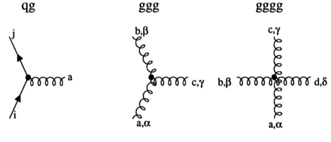
acc adFigure 21: Some CD interactions. The labels and are the quark color indices
(i, j = 1 2 3 while abc, and d are the gluon color labels = 1 2..., 8).
Interactions in CD
We can almost read-off the vertex factors from Equations 21-2.3. One thing to note, when comparing QCD with QED, is that the non-trivial Lie algebra of SU(3),
introduces an, extra term proportional to falc in Equation 22. This term is the one
that gives rise to the gluon-gluon interactions and is a direct result of the non-Abelian nature of QCD. In terms of the fundamental constant g,, we have for the physical (excluding the ghost terms) vertex factors:
ATa
qg -ig.,-y ij
ggg
_g.falV0,
2wabcd
gggg -igs ao-YP
where the V and W are functions of the leg momenta and can be found in refer-ence 19]. These interactions are diagramed in Figure 21. In our study we will encounter the first two of these interactions; the gggg coupling is out of our reach
since it is of higher order than the present (a2) calculations because at tree level,
0(e'e- - 5-jets =
(gg2)2 = 0(al).S SIn the above the jets originate from the gggg coupling with one of the legs attached
to the qV pair. More on that later.
2.2.1
Renormalization
In a Quantum Field Theory (QFT) like QCD, loop integrals are in general divergent. These divergencies are rooted in the 'locality' assumption of QFT: that interactions between two objects occur at the same space-time point (point-like interactions). However, a renornializable theory is one that allows the divergencies to be absorbed
2.2. The Theory
into the physical parameters of the Lagrangian via a finite renormalization program. As mentioned previously, CD has been shown to be renormalizable.
In order to visualize the above, it is useful to consider the case of mass renormal-ization in QED 20]. If we divide the QED equivalent of Equation 21 into a free and
interacting part,
IC = 'co Ci.t, (2.4)
and consider that electrons are stable and observable, then we would expect that S,--., (the matrix element for electron --* electron transition) should be 1. In fact, since electrons undergo self-interactions (emission and absorption of virtual photons), Se, 5 1. But we know from experience that if we "watch" an electron at the characteristic distance d ;-, F/y2 (e.g, Thompson scattering with 2 --+ 0) we can
measure a physical mass m,. So in order to recover S,-+ = for the free Lagrangian, we have to modify the decomposition in Equation 24 by adding a m term to the bare electron mass and subtract it frornCi,,t. Since we have "observed" the electron at a particular distance, this counter-term subtraction has been explicitly performed 2
at the scale Q = p,2.
This re-shuffling of terms, the renormalization procedure, is just a response to the fact that the quantities postulated in the "bare" (unrenormalized) Lagrangian do not correspond to physical observables when interactions are present. This procedure is not unique.
Dimensional Regularization
Before carrying out the renormalization procedure, the infinities of the theory must be identified and regularized. This is usually accomplished by re-writing the Lagrangian
(or any quantity being calculated) with an explicit off; in the limit that this cut-off vanishes the original expression is then recovered. Of the various regularization schemes, the most convenient one for CD is dimensional regularization 21]. This scheme is especially suited for CD as it respects gauge invariance and makes it unnecessary to introduce additional invariance-restoring counter terms. In this pro-cedure, the infinities are regulated by continuing the dimensionful expressions in the Lagrangian (and subsequent integrals) to n = 4 - 2. In order to keep the coupling g, dimensionless, the replacement g, --+ y6g, is made throughout. The arbitrary pa-rameter is not specified with the exception that it has the units of mass; thus an explicit dependence on is introduced into the rescaled g,: g = MP). The infinities are then explicitly re-expressed as poles in (1 /,,) n. Of course, at this stage nothing
has changed: the original divergent expression is still obtained in the limitE -- 0.
'This is one difference between QED and QCD: since electrons are observable, an unambiguous renormalization scale can be chosen whereas QCD offers no such free states.
CHAPTER 2 QUANTUM CHROMODYNAMICS
Renormalization Schemes and Conventions
In this section, we follow the treatment and conventions of Duke and Roberts 22] and Muta 16].
One can always write any CD perturbatively calculated observable as,
R(g = ro + r
g2 + 2 g 2(2.5)
4,x 47r
where g is the strong coupling a. = 2 /4r, and where the ri are calculable i-th order
coefficients. These coefficients (as we will see in the specific example of jet rates later) are in general ultraviolet divergent and are controlled by a specific regularization and renormalization program. We have said that renormalization amounts to a reshuffling of terms in the Lagrangian; this reshuffling can be done in a infinite number of ways. If we attach the label 'a' to both the ri and g in Equation 25 denoting one of the particular renormalization conventions, we write,
a(9a
ra'
+ ra g2+ r
ga 2 -a ( g2R 0 2 + + Vn _) (2.6)
47r 47r 47r
where we have explicitly truncated the series expansion at the n-th order. But we know that in real life observables yield definite results that do not depend on any renormalization convention. We would then expect that for a different renormaliza-tion convenrenormaliza-tion R a (9a) ;z Rb(9b)-at least to the maximum order of the calculation.
We can rephrase this by saying that assuming we have an n-th order calculation of Equation 25 available, this last requirement can be written 3 as 22],
[R(g2 /47r )]a
-
[R(g2/47r
)]b = 0([g2 /4,]n)(2-7)
n n
where n denotes the order at which the series 25 is truncated and a and b denote different renormalization schemes. We see then that as n - oo, the results of the perturbative expansions in two different renormalization conventions given by Equa-tions 25 and 26 agree. We will encounter the effects of the truncation in Equation 26 in our measurement in the form of renormalization scale uncertainties.
Examples of various renormalization conventions are given in reference 22]. In our work we choose to use the modified minimal subtraction scheme, which together with the dimensional regularization procedure, completes the renormalization program. In this scheme the 1/e poles in the perturbative expansion are subtracted via Lagrangian counter terms. he additional terms In4r - -YE' (-YE i Euler's constant), relics of the dimensional regularization, are also subtracted.
We should mention that some authors (e.g., Stevenson 23], Brodsky et al. 24],
3We also use the result 16] that the two couplings can be related through a finite renormalization transformation. This in turn implies that ro and r, are scheme independent and that the higher order ri can be converted from one scheme to another.
2.2. The Theory
among others) advocate specific schemes to reduce the renormalization scheme am-biguity that arises due to the uncalculated terms in Equation 27. The use of these schemes is generally called 'optimized perturbation theory'. The PMS scheme, for ex-ample, advocates evaluating an observable at the scale Q* such that R(g, Q*)IOQ = 0. Such a scale would presumably minimize the effects of missing higher orders by artificially reducing the sensitivity to them. Other people 14], however, have argued strongly against some of these schemes.
The -function and the Running of a,
In this section we will investigate the consequences of renormalizing the strong cou-pling g.. We will denote the bare (unrenormalized) coucou-pling by A and the
renormal-ized coupling by g,. Good references for this section are Gross and Wilczeck 25] and
Field 19].
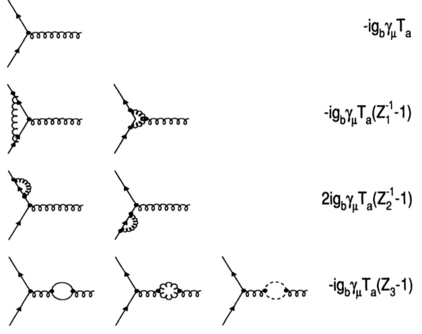
The leading order corrections to the qqg vertex are shown in Figure 22. The rightmost column in the figure shows the amplitude for the sum of amplitudes in each row. The Zi' factors are the renormalization factors 19] absorbing the ultraviolet divergencies of the corresponding amplitudes'. In order to extract the renormalized strong coupling, the corrections in Figure 22 are added to yield 19],
- ga',T.
[1
+ (Zi 1 - 2(Z
- ) + (Z3 - 1)] (igOpU
Z2 VZ3
Z2 rZ.
(-igOJ.),
(2.8)
Z,
where we can now read off the the renormalized coupling in terms of the bare coupling,
9S - Z2 NfZ3 (2.9)
Z,
The Zi are written in terms of the coupling gs, the dimensional regularization mass, A, the explicit divergent parts 1/f-, and some QCD factors. Combining these into Equation 29 to order g 2 gives 26],
g, + 2 0
+ ln(4,x -
Y_'9b,(2.10)
167r 2 c
where the above is given in the MS scheme and where,
11 2
00
N - -nf.3 3
In the above, N, = 3 is the number of colors and nf is the number of quark flavors.
'By convention, i = corresponds to the vertex correction, i = 2 corresponds to fermion self-energy corrections, and i = 3 corresponds to the gluon propagator corrections.
CHAPTER 2 QUANTUM CHROMODYNAMICS
We now impose the requirement that, since is an arbitrary parameter, A must be
independent of p, or,
d9b P 19
+ ag, a
A0-dy 0/1 9P Og"
Applying this last result to Equation 210 and performing the renormalization sub-traction gives,
ag, 00 3 (2.11)
ap
16r2
)and the renormalization group (RGE) result 27] is obtained. In this last equation, the renormalization procedure has been carried out using the MS prescription. A very important result is already evident from Equation 211. Notice that for Po > (equivalently, nf 16), Equation 211 implies that the coupling g, decreases with an increase in the energy scale. This very important property is called asymptotic freedom and allows us to use perturbation theory at high energies in CD. It is important to note that this behavior ('negative -function') is solely due to the non-Abelian nature of QCD (cf., QED has a 'positive -function').
Writing Equation 211 to higher orders 28] and using a. = g,2/47r, we quote,
i9a, floa2 _ pi a 3 (2.12)
19P 2r 8r2 8
where 0 = 102 - 3' nf and where the right side of the above equation is generally called3 the -Junction. The coefficients 00 and 1 are renormalization scheme independent; in general, however, higher order coefficients do depend on the renormalization scheme
used.
Perturbative QCD does not tell us the 'absolute value' of a, it just tells us how it behaves through Equation 212. In fact, what is missing from the differential equation, and is not given by the theory, is a boundary condition to completely specify the behavior of a,. In QED the Thompson limit Q 2 --+ 0) provides a natural
boundary condition defined in terms of an observable object-an electron. In QCD the convention 6] is to introduce a renormalization scheme dependent mass parameter
A,
Q2 (Q) dx
In (2.13)
A 2 OW,
where is the function defined by Equation 2.12. In the following, and for sim-plicity, the one-loop approximation (Equation 211) will be used. One can see from Equation 213 that the chosen boundary condition is a,(A = oo.
We can proceed with Equation 213 to obtain a closed form for ,,
47r
a., (Q = #o ln(Q2/A2)'
(2.14)
2.2. The Theory
-'MJa
-igJja(Zi
-1-1)
2igbyRT.(Z-1 - ) 2-
It-"
-igbyja(Z3-1)
Figure 22: Leading order corrections. Top to bottom: the bare vertex, vertex correction, quark self-energy correction, and gluon propagator corrections. Lines are quarks, wavy lines are gluons, and dashed lines are ghosts. 9b stands for the bare coupling and T"
is the SU(3) generator.
We now see the role of the QCD parameter A: it acts as a vague limit at which a, becomes strong, and it sets the scale at which a, 'runs' (i.e., 'how fast' it runs). it is this parameter which we will determine in this analysis.
It is instructive to paint a physical picture of asymptotic freedom. In QED, the vacuum polarization (virtual ee- pairs) shields the bare charge eb into a renormalized charge e(Q = 0), defined at large distances. As one probes this polarization cloud
(Q 2 --+ 00), this screening effect becomes less pronounced and we see a larger effective
charge. In QCD the reverse is true. We still have color charge screening due to q vacuum polarization, however, now the gluons also carry charge. This means that our test particle (the 'source' of color charge) can now radiate its charge away. As
we get closer to it, this radiation becomes more prominent and we have less of a chance of localizing the original test charge. Thus, the effective color charge in QCD become weaker as Q --+ oc. We may be tempted to extend this picture to the confinement limit ut in that limit our picture of single gluons and charges breaks down (non-perturbative regime).
CHAPTER 2 QUANTUM CHROMODYNAMICS
Some Results We'll Need
Before leaving this section, we will quote some results which will be used later in the analysis. The second order solution (next-to-leading order) to the -function is 28],
12ir 6(153 - 19nf) In[In(Q2 /A 2)]
a,, Q = 1 - (2.15)
(33 - nf )
ln(Q2/A2)(33 - 2nf)2
ln(Q2/A2)where, again, we will use A = AVS-. An alternative solution to Equation 212 with the -function truncated at second order is 28],
go In /I = 1 + pi In a, W (2.16)
27r A a.(,u) 4,x Po a, (P) + 4rOo
91
which enables us to easily present the results in terms of AWS-. Equations 215 and 216 are equivalent to (a2) and may thus be used interchangeably; however, one must be careful in being consistent in their usage. The conversion between AWs- from Equations 215 (labelled W) and 216 (labelled 'B') is,
AA = 1.076AB7 (2.17)
where A = AVS- is for five active flavors.
One may freely convert the A parameters between different renormalization schemes and different number of flavors. Two renormalization schemes are related by a Moop calculation 6 By imposing continuity at the boundary conditions of the flavor thresholds in Equation 215, the AWS- for different nf can also be calculated 29].
It is important to note that in order to have a meaningful determination of A, at least a next-to-leading order calculation must be used 30]. The reason is that to leading order (Equation 214) a scale change in A of 0(l) implies a change in a,
of (a2). Thus to leading order, a determination of A yields an effective Aff not
related to the parameter of the theory As,
2.3 Perturbative
CD in ee- Annihilation
2.3.1 Experimental Developments
The annihilation of e+e- provides a very clean environment for QCD studies. A nice feature of such colliders is that the center of mass system, except for initial state radiation, coincides with the laboratory reference system, making the job of untangling final states much easier.
The most direct, manifestation of quarks or gluons in a quasi-free state is jets. In 1970, while considering various models for hadron distributions in e- annihilation,
2.3. Perturbative CD in e- Annihilation
Bjorken and Brodsky 31] suggested the idea of "jets" as a possible manifestation of the parton structure of a heavy virtual photon. It was five years later, a the
Mark II detector at SPEAR 32], that the first evidence for jets was obtained by observing an excess of low sphericity events at ,z- 7 GeV. In addition, from the 1 Cos 20 distribution of the sphericity axis of the hadronic events, it was inferred
that the produced quarks were spin-1 objects. This was a great triumph for 2 CD; in a completely different environment from the DIS experiments, it had been shown that spin- quarks were observable in the asymptotic limit.2
The observation of gluon emission came later in 1979 33]. Three jet events were observed in the experiments at the PETRA ring in DESY at an energy s - 30 GeV. This time, the separation of three-jet events from phase-space distributed events proved more difficult than with two-jet events. The problem was that it was no longer sufficient to separate the events into hemispheres - there was an ambiguity in defining
the third jet. The fragmentation process was smearing the initial parton direction
and thus made it impossible, on an event by event basis, to differentiate a true gluon jet from a fluctuation in the hadronization. This could only be shown statistically.
We still suffer from these hadronization effects. The smearing introduced by such effects and our lack of knowledge of these JOWQ2 phenomena will introduce a
sys-tematic uncertainty in our measurement of jet-rates. These effects will be discussed in more detail later.
2.3.2
CD Perturbative Predictions
In this section we will briefly motivate and review the O(a 2) .9 matrix element
calcu-rations with the purpose of setting the stage for the actual measurement. Very good
references for perturbative CD are Kramer 26] (PQCD in ee-) and Muta 161
(PQCD in general). We will closely follow Kramer's treatment.
Some ee-
CD Quantities
In ee- annihilation one can vaguely classify, in an experimental sense, 'a,-dependent' quantities as either being inclusive or kinematically distributed quantities. Example of inclusive observables are [5]:
• Re+e-: hadronic fraction of the total cross section
• Fh/171: the hadronic/leptonic fraction
• R,: hadronic fraction for leptons
By being inclusive, the measurement of the above quantities is fairly insensitive to the final state. For example, hadronization effects are especially suppressed. In addition,
CHAPTER 2 QUANTUM CHROMODYNAMICS
the available calculational techniques allow calculations of up to 0(a' ), making the
above attractive candidates for the determination 6 of a. However, the dependence
on a, (in the above variables) enters as a QCD correction, and although known to third order, tends to be dominated by statistical errors.
Some examples of kinematically distributed quantities 34] are: * Event shapes: thrust, oblateness, heavy jet mass
e Particle-inclusive quantities: energy-energy correlations (EEC), asymmetry of the EEC (AEEC), single particle spectra
* Jet quantities: jet rates, differential jet rates
The above observables are defined either in terms of single particles or in terms of clusters of particles. This implies, of course, that fragmentation uncertainties dilute the measurement. In addition, none of these quantities have been fully calculated to higher than O(a') so far and thus the maximum achievable accuracy is less than for the inclusive quantities. Therefore, in general, inclusive quantities have smaller
theo-retical uncertainties than kinematically distributed quantities. There is one important
advantage over the inclusive variables, though; the above quantities can in general be written as direct proportionalities with a,. Thus the experimental sensitivity is much higher.
From now on we will concentrate on the jet related quantities. We will briefly review the calculation of gluon radiation in e- annihilation and use it to predict jet rates. The fact that this prediction is a function of a, will enable us to use it later on to extract a value of AVS- from the data.
The Parton Final States to 0(a,)
It is instructive to outline the issues involved in the calculation of qqg final states in e+e- annihilation to O(a,). These issues are representative of the ones encountered in the higher order calculations but are less encumbered by the algebra.
Up to O(a,), we can have at most three partons in the final state. The complete set of Feynman diagrams that contribute to this order are shown in Figures 1-1 and 2-3a (qq tree level and I-loop) and in Figure 2-3b (qqg tree level). Each diagram in 2-2-3a carries an ultraviolet (k --+ oo) divergence that cancels when the three diagrams are added. An additional divergence, this time infrared (k - 0), appears due to the masslessness of the gluons. However, the diagrams of Figure 2-3b display the same divergence with the opposite sign and thus cancel it in their sum. There is still one more related divergence to discuss but we first turn our attention to the nature of the cross section.
2.3. Perturbative
CD in ee- Annihilation
- --- ----a)
I---b)
Figure 23: Diagrams contributing to 0(a,,) parton production. a) shows the 2-parton
final state virtual corrections and b) shows the 3-parton final state at tree level.
An essential reference for the following is Appendix A, where the kinematic conventions are established. We define xi as the scaled energy of each parton, xi = 2EilE,,,,, with x, > X2 > X3 and X1 + X2 + X = 2 Since we only have
three partons in the final state, the kinematics leaves us with only two independent variables which we take to be x, and
X2-20 1 2
to
o9 a 1 7 < 5 Y23 coffinear Y. 4 ! -k&ired Y13 3 I . I I . , , I . . I . . . . , I collinear 2 10 Q, (in GeV)Figure 24: The phase space region for 3 parton final states, including the infrared and collinear regions.
Figure 25: Average number of partons
as a function of the parton shower virtuality cutoff Q.
CHAPTER 2 QUANTUM CHROMODYNAMICS
known result 35], 2 A &a a, xi 2 = CF (2.18)dxdX2
2r ( - x)(1-
X2)'where a, is the lowest order qq cross section at the Z, given by Equation 12, and CF= 43 is the appropriate color factor for this color configuration. Notice that the above exhibits the explicit gluon mass singularity (for x, andX2 -+ 1) since it does not have the virtual corrections added.
Eventually we will see that what allows us to make inferences about the rate of hard gluon radiation is the good (asymptotic-free justified) approximation that hadron jets correlate to the initial 'color-full' partons. With this in mind, we now shift our focus and treat Equation 218 as the 3-jet cross section formula (again,
just to 0a.)). But we immediately notice that for very soft gluons (say, X3 -- * 0),
we go into the 2-jet limit X = X = 1) and Equation 218 diverges. This is no
surprise; we already noticed this gluon infrared divergence and remarked that it was cancelled with the virtual corrections of Figure 2-3a. However there is still a collinear divergence associated with the assumption of massless quarks'. Also, since we are not just interested in att, we ought to have a consistent procedure to separate and define the 3-jet events.
This last task is accomplished by dimensionally regularizing the virtual and real parts of the cross section and by partitioning the phase space of the q-g events into 'distinguishable 3-jets' and 3-jets 'indistinguishable from 2-jets'. This last category is then absorbed into the 2-jets for a particular cut-off of the 3-jet phase space. Following the convention of Appendix A, we define in terms of the invariant yij the 3-to-2 jet boundaries in Figure 24. We label the boundary 4YC ) or Ycut'- Remembering
that Y23 = - xi, we see that the shaded rectangular regions correspond to the
collinear divergent parts of Equation 218 and that the heavily shaded square region corresponds to the infrared divergent part.
The shaded areas of the qqg phase space in Figure 24 correspond to the areas where two of the partons are unresolvable. In this region the 3-jet events are indis-tinguishable from the 2-jet events. Rewriting Equation 218 in terms of the invariant measure , dimensionally regularizing it, and integrating over the 2-jet bands 26], one obtains:
or2 4irp 2 a, (y2) CF E)
3-3et(Y' < Yc) q
S
2r
r(l - 2c)
2 3 2 72 +
X + 2 In YC + 4yc In y 7 (2.19)
E2 E 3
In the above, oq is given by Equation 12 and is the arbitrary mass scale introduced to keep the coupling constant dimensionless in generalized n = 4 - 2E dimensions.
7This comes about through cos q I in m 2 = Eq E. (I cos Oqg) terms in the quark propagator
2.3. Perturbative
CD in ee- Annihilation
The subscript and superscript on the left-hand side denote that Equation 219 is the cross section for resolving 2-jets from a 3-parton configuration.
Doing the virtual and real integration for the 2-parton final state to 0(a.) using the diagrams of Figure 2-3a and 1-1 yields,
2-jet 47ru 2 f a,
W) r(i C)
2 3 27r2Or2 aq CF __
+
8
(2.20)
S 27r IF(l - 2c) 62 f 3
where the subscript 2 in the left hand side stresses the fact that the cross section derives from the two parton final states. Notice that Equation 220 has no depen-dence since initial two-parton states will always be resolved as 2-jets. Now it is also clear what we meant by saying that the divergencies would cancel when all diagrams
were taken into account: when adding Equations 219 and 220 to obtain the total
2-jet cross section, the infrared and collinear pole terms 1/ E 2and 16 respectively) cancel in the sum. After this summation, we take the e --* limit to recover four dimensions, and we write for the total 2-jet cross section,
a2-Jet 2 YC) + or 2-jet (2.21)
2+3 (Y < YC) = Or3_"t(Y < 2
2 3
= aq 1 + 2r
CF-21n YC
- 31ny, + 4yclny - 3 where now the 2-jet cross section depends on the resolution parameter y, that deter-mines when 3-jet events are distinguishable from 2-jet events. We should mention that the accuracy of these calculations in the low-y region has been extended recently 36] by partially resumming the next to leading logarithm terms (a' In' y terms above)8 in the jet rate calculations. These methods increase the measurement accuracy some-what by reducing the renormalization scale dependence (e.g., See Table 69).The above cancellation of infrared and collinear divergencies when integrating the cross section over regions of phase space where the final states are unresolvable is a specific example of the Kinoshita-Lee-Nauenberg (KLN) theorem 37]. The theorem is a general result for degenerate states': infrared and collinear divergencies cancel in a theory with massless fields when a summation is performed over degenerate states. This theorem holds to all orders in perturbation theory.
As a final comment, it should be pointed out that Equation 218 can be generalized to calculate some of the QCD observables discussed previously. However, in order to satisfy the KLN theorem and obtain sensible cross sections, these observables must respect the degeneracy of the soft and collinear partons. This means that in general good observables are linear in parton momenta (see Appendix A). Observables that satisfy these requirements are said to be infrared and collinear safe 38].
'Two massless collinear partons are degenerate because they can be treated as a single parton. The same applies to infrared degeneracy-when a parton accompanied by a very soft gluon can be combined into one parton.
CHAPTER 2 QUANTUM CHROMODYNAMICS
The (a2) Result: the ERT Calculation
Now that we have presented an outline of the 0(a,) calculation, we turn our attention to the (a2) results. The a (a2) calculation has been performed by various groupsa (e.g., 39, 40]) In our measurement we will use the calculation by Ellis, Ross, and Terrano (ERT) 39]. The ERT calculation has been done for different jet algorithms with different recombination schemes. This last issue is a technical point that we will address in Chapter 6.
In the previous section we saw that we were able to calculate the 3-jet cross section without recurring to any renormalization technique. The reason was that we did not encounter any persistent ultraviolet divergence; all the divergencies conveniently
0 2)
cancelled when the appropriate accounting of diagrams was performed. In the as case however, we encounter diagrams with persistent divergencies (the loop diagrams
to O(a2)) that require a renormalization procedure. In the following, and for the rest of this work, the modified minimal subtraction renormalization scheme (VS-) will be used. The QCD parameter A will be,
AQCD = Anf Ms--5 (2.22)
where the superscript denotes five active flavors.
The ERT result can be conveniently expressed 34, 36] as,
O'2 Y)
R2 (Y, P -
A(y)
- (B(y, f) + C(y))
01tot 27r 27r
0'3 (Y)
R3 (Y, - =
A(y)
+ B(y, f)
01tot 27r 27r
0'4 (Y)
R4 (Y, Y - = C(Y) 1 (2.23)
01tot 2r
where y = y, and where, for example, 0'2(y) has the same meaning as in Equation 221 except that it is one order higher in as. The total cross section in Equation 223, O'tot, is the one given by Equation 1.1 to at least (a2). The leading order terms AS and C depend on y only while the next-to-leading term depends on y and on the
renormalization scale f = 2/Q2,
B (y, y = BY' Q2) + A(y)27rpoln(f).
(2.24)
In the above, 0 = 1 - 2nf /3 and nf is the number of active quark flavors.
Experimentally, the Ri(y,) above are calculated by classifying and counting events as i-jet events at y = y, and then normalizing this number to the total number of events. In practice the functions A(y), B(y, f), and C(y) are tabulated from Monte
Carlo integrations of the cross sections 34] and then parameterized as a sum of simple