Book Physics Laboratory Manual pdf - Web Education
Texte intégral
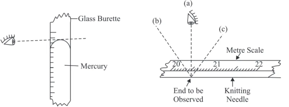
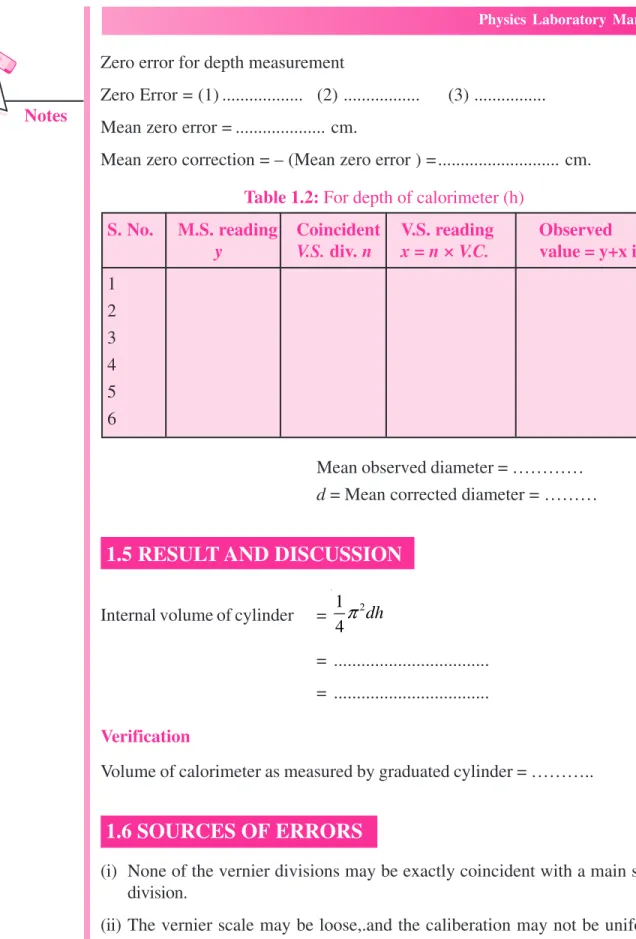
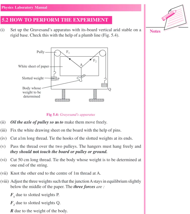
Figure


Documents relatifs
the components of a position vector with respect to a coordinate system, the scalar product of two vectors, the transformation of the components upon a change of the coordinate
We discussed quantum tunnelling in Chapter 2, where we saw that wave- particle duality means that particles such as electrons can penetrate a potential barrier where this would
The adequate framework is given by quantum electrodynamics, a quantum field theory, which combines classical electrodynamics and relativistic quantum mechanics. By subtracting
Consider a spherical electromagnetic wave propagating with a speed c with respect to a stationary frame of reference, as shown in figure 1.9.. The speed
It is because of these properties that Hermitean operators place a central role in quantum mechanics in that the observable properties of a physical system such as posi- tion,
Some textbooks assign a magnetic charge (also called pole strength) +q m to the north pole and –q m to the south pole of a bar magnet of length 2l, and magnetic moment q m (2l)..
For example, the Hydrogen atom in three dimensions has 3 coordinates for the internal problem, (the vector displacement between the proton and the electron). We will need three
In each case, draw the angle and its supplementary and vertically opposite angles in the same figure mentioning their degrees.. Mark also the vertically opposite angle of
