HAL Id: hal-03185772
https://hal.archives-ouvertes.fr/hal-03185772
Submitted on 30 Mar 2021
HAL is a multi-disciplinary open access
archive for the deposit and dissemination of
sci-entific research documents, whether they are
pub-lished or not. The documents may come from
teaching and research institutions in France or
abroad, or from public or private research centers.
L’archive ouverte pluridisciplinaire HAL, est
destinée au dépôt et à la diffusion de documents
scientifiques de niveau recherche, publiés ou non,
émanant des établissements d’enseignement et de
recherche français ou étrangers, des laboratoires
publics ou privés.
V. Wakelam, P. Gratier, M. Ruaud, R. Le Gal, L. Majumdar, J.-C. Loison, K.
M. Hickson
To cite this version:
V. Wakelam, P. Gratier, M. Ruaud, R. Le Gal, L. Majumdar, et al.. Chemical compositions of
five Planck cold clumps. Astronomy and Astrophysics - A&A, EDP Sciences, 2021, 647, pp.A172.
�10.1051/0004-6361/202039367�. �hal-03185772�
Astronomy
&
Astrophysics
https://doi.org/10.1051/0004-6361/202039367
© V. Wakelam et al. 2021
Chemical compositions of five Planck cold clumps
V. Wakelam
1, P. Gratier
1, M. Ruaud
2, R. Le Gal
3, L. Majumdar
4, J.-C. Loison
5, and K. M. Hickson
5 1Laboratoire d’astrophysique de Bordeaux, Univ. Bordeaux, CNRS, B18N, allée Geoffroy Saint-Hilaire, 33615 Pessac, Francee-mail: valentine.wakelam@u-bordeaux.fr 2 NASA Ames Research Center, Moffett Field, CA, USA
3Harvard-Smithsonian Center for Astrophysics, 60 Garden St., Cambridge, MA 02138, USA
4School of Earth and Planetary Sciences, National Institute of Science Education and Research, HBNI, Jatni 752050, Odisha, India
5Institut des Sciences Moléculaires (ISM), CNRS, Univ. Bordeaux, 351 cours de la Libération, 33400 Talence, France Received 8 September 2020 / Accepted 29 January 2021
ABSTRACT
Aims. Interstellar molecules form early in the evolutionary sequence of interstellar material that eventually forms stars and planets. To
understand this evolutionary sequence, it is important to characterize the chemical composition of its first steps.
Methods. In this paper, we present the result of a 2 and 3 mm survey of five cold clumps identified by the Planck mission. We carried
out a radiative transfer analysis on the detected lines in order to put some constraints on the physical conditions within the cores and on the molecular column densities. We also performed chemical models to reproduce the observed abundances in each source using the gas-grain model Nautilus.
Results. Twelve molecules were detected: H2CO, CS, SO, NO, HNO, HCO+, HCN, HNC, CN, CCH, CH3OH, and CO. Here, CCH is the only carbon chain we detected in two sources. Radiative transfer analyses of HCN, SO, CS, and CO were performed to constrain the physical conditions of each cloud with limited success. The sources have a density larger than 104cm−3and a temperature lower than 15 K. The derived species column densities are not very sensitive to the uncertainties in the physical conditions, within a factor of 2. The different sources seem to present significant chemical differences with species abundances spreading over one order of magnitude. The chemical composition of these clumps is poorer than the one of Taurus Molecular Cloud 1 Cyanopolyyne Peak (TMC-1 CP) cold core. Our chemical model reproduces the observational abundances and upper limits for 79–83% of the species in our sources. The ‘best’ times for our sources seem to be smaller than those of TMC-1, indicating that our sources may be less evolved and explaining the smaller abundances and the numerous non-detections. Also, CS and HCN are always overestimated by our models.
Key words. astrochemistry – methods: observational – ISM: abundances – ISM: clouds – ISM: molecules
1. Introduction
Star and planet formation is the final step in a long sequence of interstellar matter evolution that starts from the diffuse medium. The first step, that of condensation, which sees the formation of cold cores, is not a well-constrained phase. The formation time and the evolution of the physical conditions are probably very variable, depending on the processes at work. From an observa-tional point of view, cold cores are small (0.03–0.2 pc), dense (104–105 cm−3), and cold (8–12 K) starless sources (Bergin &
Tafalla 2007). They are located within clumps (typical sizes of 0.3–3 pc), which are themselves located within clouds (2– 15 pc). In these shielded regions, the gas and dust temperatures are expected to be below 20 K and the UV photons produced by surrounding massive stars cannot penetrate. Consequently, chemistry produces molecules that can survive, although they will be mostly trapped in icy grain mantles. One key issue is determining what level of complexity interstellar molecules are able to reach at this stage. A recent observation of
com-plex organic molecules (Bacmann et al. 2012;Cernicharo et al.
2012;Vastel et al. 2014) in the gas-phase in these objects indi-cates that molecular complexification could begin much earlier than previously thought. Reproducing this chemical complex-ity is still challenging for astrochemical models in which many chemical parameters, but also the processes themselves, are not
well-constrained (Wakelam et al. 2010). Sometimes, even the
abundances of the more basic species can be difficult to under-stand, particularly when the observational values published in the literature are in disagreement. Taking the example of CN, there are two abundances for this molecule in TMC-1 (CP) reported in the literature with a ratio of nearly 40 between them (Crutcher et al. 1984; Pratap et al. 1997). Such disagreements can be attributed to the use of different telescopes, spectroscopic data, radiative transfer assumptions (local thermodynamic equi-librium, optical depth) etc.
From a general point of view, few sources exist for which a complete chemical survey, using coherent methods, have been performed. As far as we know, only two starless cold cores have been extensively studied thus far: TMC-1 (CP) and L134N (N). TMC-1 (CP) refers to the ‘Cyanopolyyne Peak’ within the
Taurus molecular cloud (Pratap et al. 1997; Ohishi & Kaifu
1998) while L134N (N) refers to the ‘North Peak’ in the isolated
core L134N (also called L183; Dickens et al. 2000).
Abun-dances observed in these two clouds have been compiled from
the literature byAgúndez & Wakelam (2013). These two cold
cores present significant chemical differences, particularly with respect to carbon chains, which are much more abundant in TMC-1 than in L134N. The nature itself of L134N is, however,
unclear as it might already be in the pre-stellar phase (Pagani
et al. 2004).
In this study, we present a 2 and 3 mm spectral survey of a selection of five cold clumps from the Planck Early Release
A172, page 1 of28
Table 1. Observed sources.
PlanckClump’s name PGCC RA and Dec Observed RA and Dec Labelled name
(J2000) (J2000) G153.34-08.00 03:48:41.80 +44:09:14.0 03:48:43.30 +44:07:45.0 C1 G156.92-09.72 03:57:30.00 +40:33:52.0 03:57:30.82 +40:34:22.0 C2 G157.12-11.56 03:51:58.80 +39:02:20.0 03:51:58.12 +39:00:31.0 C3 G160.53-19.72 03:38:57.70 +30:39:17.0 03:39:02.50 +30:41:30.0 C4 G173.60-17.89 04:32:50.26 +23:21:57.8(a) 04:24:38.79 +23:23:51.0 C5
Notes. (a)This source is not in the PGCC catalogue, so we report the coordinates from the ECC Planck catalogue here.
Cold Core (ECC, Planck Collaboration XXII 2011) catalogue.
Using the detected lines, we tried to constrain the physical con-ditions within the observed sources and determine the molecular
column densities (Sect.2). In Sect.3, we compare the observed
values within the different cores and with the TMC-1 (CP)
val-ues. Section4presents a chemical model for each source. Finally,
we offer a summary and our conclusions. 2. Sources and observations 2.1. Selected sources
To select the regions we intended to observe for the purposes
of this study, we used the Planck Early Core catalogue (Planck
Collaboration XXII 2011) and the follow-up mapping byMeng et al. (2013) of many of these sources in 12CO, 13CO, and
C18O. The sources presented in the Planck catalogue are quite
large, appearing more similar to clumps rather than individual
cores due to the Planck spatial resolution (∼4.40 full width at
half maximum – FWHM). They are, however, very likely to be
cold and quiescent (Wu et al. 2012). The clumps were selected
within the sample from Meng et al. sample using several
differ-ent criteria: large densities (a few 103 cm−3), large masses, low
temperatures, originating from various regions of the sky, and be detected in the three CO isotopologues. The selected clumps are G153.34-08.00, G156.92-09.72, G157.12-11.56, G160.53-19.72,
and G173.60-17.89 (see Table 1 of Meng et al. 2013). Within
these clumps,Meng et al.(2013) found several sub-structures in
CO. Here, we do not use the exact positions of the sub-cores
identified byMeng et al.(2013). Instead, for each of the clumps,
we used the maximum13CO(1–0) integrated intensity maps. The
pointing positions for each of our clumps are summarised in
Table1. For simplicity, we have labelled the observed sources
from C1 to C5. The first three clumps (C1 to C3) are located
in the California Molecular Cloud (CMC; Lada et al. 2009),
C4 is in the Perseus Molecular Cloud (PMC), while C5 is in the Taurus Molecular Cloud. These three clouds are located at
approximately 140 pc for Taurus (Dame et al. 1987), 235 pc for
Perseus (Lombardi et al. 2010), and 450 pc for California (Lada
et al. 2009).
After our observations were complete, the Planck catalogue was revised (using more sophisticated numerical modelling and combining other highest frequency channels of Planck) and the
Planck Catalogue of Galactic Cold Clumps (PGCC) was
pub-lished (Planck Collaboration XXVIII 2016). The central
posi-tions of the clumps were modified and some of the previously identified clumps were removed because they did not satisfy the compactness criterion. In particular, G173.60-17.89 is among the clumps that are not present in this catalogue. These clumps, however, have sizes of a few arc minutes, which is much larger than the difference between our position and the new Planck
catalogue positions. Herschel observations are not available for these positions. So we could not better identify the positions of the cores, if there were any at all.
2.2. Observations
The observations were taken with the Institut de RadioAs-tronomie Millimétrique (IRAM) 30 m telescope, where the data were acquired in a single 55 h observing run in April–May 2016. The Eight MIxer Receiver (EMIR) 3 and 2 mm receivers were tuned at 28 distinct frequencies to enable a nearly continuous coverage of the 3 mm (between 71.8 and 116.2 GHz) and 2 mm bands (between 126.8 and 164 GHz) at a frequency channel spacing of 48 kHz (corresponding to velocity channel spacing
ranging from 0.09 to 0.2 km s−1). The observing conditions were
very good, with typical system temperatures of 120 K at 3 mm and 150 K at 2 mm, which enabled us to reach a typical noise level of 8 mK at 3 mm and 18 mK at 2 mm.
The five sources were observed using position switching with an OFF position selected for each source having minimal
emis-sion in theMeng et al.(2013) CO maps. Contamination from the
‘off’ is only present for the12CO lines in sources C2, C3, and
C4 but at different velocities. Primary pointing and focus were done on Mercury and secondary focus was achieved on quasars 0316+413, 0355+508, 0430+052. The average pointing correc-tions were between 300and 400(4 times smaller than the 1500beam
at 164GHz). The beam size was between 3500 (at 72 GHz) and
1500(at 164 GHz).
2.3. Data reduction
Data reduction, line identification, and line fitting were
car-ried out using the CLASS/GILDAS package (Pety 2005)1. The
spectroscopic catalogue used for line identification is the JPL
database2and the CDMS database3(Müller et al. 2005). Within
the observed frequency ranges, 12 molecules were detected in at least one of the sources, plus one isotopic line of CS and
of HCO+, and three isotopic lines of CO. The list of detected
molecules and lines (with spectroscopic information and the
crit-ical density of the lines at 15 K) is given in Table A.1. The
observed spectra for these lines are given in Figs.B.1–B.5. The
Gaussian line fit parameters for all detected lines in each of the
five sources are given in TablesA.3–A.7. An absence of line
parameters means that the lines were not detected and in that case, we just give the noise level. The 3σ upper limits on the inte-grated intensities were computed assuming a Gaussian shape and
a line width of 1 km s−1similar to the typical line width detected
1 http://www.iram.fr/IRAMFR/GILDAS/ 2 https://spec.jpl.nasa.gov/
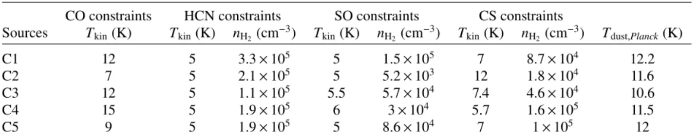
Table 2. Physical properties of the sources.
CO constraints HCN constraints SO constraints CS constraints
Sources Tkin(K) Tkin(K) nH2(cm−3) Tkin(K) nH2(cm−3) Tkin(K) nH2(cm−3) Tdust,Planck(K)
C1 12 5 3.3 × 10⁵ 5 1.5 × 10⁵ 7 8.7 × 10⁴ 12.2
C2 7 5 2.1 × 10⁵ 5 5.2 × 10³ 12 1.8 × 10⁴ 11.6
C3 12 5 1.1 × 10⁵ 5.5 5.7 × 10⁴ 7.4 4.6 × 10⁴ 10.6
C4 15 5 1.9 × 10⁵ 6 3 × 10⁴ 5.7 1.6 × 10⁵ 11.5
C5 9 5 1.9 × 10⁵ 5 8.6 × 10⁴ 7 1 × 10⁵ 12
for the other molecules in these sources with the CASSIS
software4 (developed by IRAP-UPS/CNRS), providing the
pro-duced line does not go above three times the rms. All temper-atures given here are main beam tempertemper-atures. In the observed spectral range, we expected to detect more types of molecules,
such as carbon chains. Table A.2 lists these molecules and
the spectroscopic information of the lower energetic transition present in the observed frequency range.
Looking at the number of detected lines and line intensi-ties, the five clouds present significant differences. In C2, for instance, only half of the molecules were detected, whereas in C3, there is only one molecule that was not detected. CCH is detected only in C1 and C4, while NO and HNO are only detected in C3. CS, SO, HCN, HNC, and CO are detected in all five sources. The lines in C4 have a larger width than in the
other sources and present a double peak in 13CO, CS, H
2CO,
HCN, HCO+, HNC, and SO. The 12CO line in C4 does not
have a double peak but shows a strong redshifted wing. The presence of wings or multiple peaks in the emission lines of
Planck’s cold clumps have been discussed byMeng et al.(2013)
andLiu et al. (2019), where it is often interpreted as a signa-ture of multi-components in the line of sight, which may then be
the case for C4. Furthermore,12CO in C3 and C5 also present
a small double peak profile but since none of the other species (including isotopic CO) have it, we assume that this is due to an
optical depth effect. Molecules such as HC3N and C3H2were not
detected in any of the observed sources. For the lines presenting a double peak, we checked that the integrated intensity obtained with a single Gaussian profile does not change significantly as compared to a fit with two Gaussians.
2.4. Method of analysis and observational constraints 2.4.1. Physical conditions in the clumps
Our analysis of the molecular content of these clumps is lim-ited by the small number of lines detected for each species. As an attempt to constrain the physical conditions in each of
the clumps, we first use the 12CO observed line intensity to
determine the gas kinetic temperature assuming that the line is optically thick and the source is filled in the beam (see e.g.
Eq. (1) ofMeng et al. 2013). The assumption that the sources
fill the beam may not be correct as we will discuss later in
the paper. Table2 contains our computed kinetic temperatures
derived from12CO. When compared to the study ofMeng et al.
(2013), we found that the observed peak intensities of CO are
larger in our sample in many cases and sometimes by a factor of 3. This could be an effect due to beam dilution if the sources do not fill the beam as our beam is smaller than theirs. This could also be the consequence of a different selected position of the sources. For C2 however, we have the same position as their
4 http://cassis.irap.omp.eu
G156.92-09.72C1 (see their Table 4). At this position, our12CO
intensity is 21% smaller than theirs and we have a similar13CO
intensity, however, our C18O intensity is twice as large. Because
we have different CO intensities, our gas kinetic temperatures derived from CO are different – and in most cases, smaller.
To independently derive a kinetic gas temperature and a total hydrogen density, we studied the excitation conditions of
HCN, SO, and CS using χ2minimisation scripts in CASSIS with
the RADEX5 model (van der Tak et al. 2007), assuming
non-LTE conditions and a homogeneous slab. The χ2 values were
computed by fitting the full line profiles to synthetic spectra.
Non-detected lines are also considered for the χ2calculation. We
varied the gas density, the kinetic temperature, and the species
column densities in the ranges (5 × 10³–5 × 105cm−3), (5–15
or 20 K), and (1012–5 × 1014 cm−2), respectively, with regular
grids of 30 points each. We used the collisional coefficients from
Hernández Vera et al.(2017) for HCN,Lique et al.(2007) for SO, andDenis-Alpizar et al.(2013,2018) for CS. All three are defined down to 5 K. For HCN, the detection of the hyperfine component of the 1–0 line and the non-detection of the 2–1 line provide strong constraints. For CS, two lines were detected in almost all sources, while for SO, only two lines (namely, the less energetic ones) were detected but there are seven lines in our sample (with upper energies up to 30 K). For each molecule, we obtained a 3D
matrix of χ2for a grid of 30 × 30 × 30 values of temperature, gas
density, and molecular column density. The ’best’ physical con-ditions (and column density for these molecules) are determined by taking the position in the three-dimensional (3D) parameter space for which the global χ2is the smallest (i.e. the likelihood is
maximal). The determined physical conditions obtained with the
three molecules in the five sources are summarised in Table2. In
order to devise a visualisation of the constraints on the physical conditions given by the line analysis, we summed the likelihood over all column densities (N) to get a two-dimensional (2D) map of the χ2 for (nH
2, T) taking into account the uncertainty on N.
Figure1shows the 1, 2, and 3σ confidence levels as a function
of the gas density and temperature. Similarly, Figs.C.1andC.2
show the χ2 contours projected over the temperatures and gas
density respectively (see AppendixC). We note that when
sum-ming the likelihood over one the parameters, the maximum
likelihood (or minimum χ2) may correspond to different values
of parameters than the global optimum over the full parameter space spanned by the 3D matrix. When we sum the values over the column densities axis, however, the values of the best param-eters are identical for the 2D and 3D case. For comparison, the dust temperatures from the PGCC catalogue are listed in the last
column of Table2.
Temperature constraints given by SO and HCN are rather strong towards very low temperatures while the constraints given
4.0 4.5 5.0 5.5 nH2 6 8 10 12 14 T CS in C1 4.0 4.5 5.0 5.5 nH2 6 8 10 12 14 16 18 20 T SO in C1 4.8 5.0 5.2 5.4 5.6 nH2 6 8 10 12 14 16 18 20 T HCN in C1 4.0 4.5 5.0 5.5 nH2 6 8 10 12 14 T CS in C2 3.0 3.5 4.0 4.5 nH2 6 8 10 12 14 16 18 20 T SO in C2 4.8 5.0 5.2 5.4 5.6 nH2 6 8 10 12 14 16 18 20 T HCN in C2 4.0 4.5 5.0 5.5 nH2 6 8 10 12 14 T CS in C3 4.0 4.5 5.0 5.5 nH2 6 8 10 12 14 16 18 20 T SO in C3 4.8 5.0 5.2 5.4 5.6 nH2 6 8 10 12 14 16 18 20 T HCN in C3 4.0 4.5 5.0 5.5 nH2 6 8 10 12 14 T CS in C4 4.0 4.5 5.0 5.5 nH2 6 8 10 12 14 16 18 20 T SO in C4 4.8 5.0 5.2 5.4 5.6 nH2 6 8 10 12 14 16 18 20 T HCN in C4 4.0 4.5 5.0 5.5 nH2 6 8 10 12 14 T CS in C5 4.0 4.5 5.0 5.5 nH2 6 8 10 12 14 16 18 20 T SO in C5 4.8 5.0 5.2 5.4 5.6 nH2 6 8 10 12 14 16 18 20 T HCN in C5
Fig. 2.13CO spectrum (in main beam temperature) observed in C1 in black and theoretical spectra at LTE in red for a kinetic temperature of 5 K and a column density of 2 × 1016cm−2.
by CS are weaker because of the degeneracy between
tempera-ture and density (see Fig. 1). Although the χ2 contours seem
to indicate that temperatures could be smaller than 5 K, the collisional rates of these molecules are not defined below this temperature, so it would be risky to extrapolate them. Such
low temperatures have already been found by Padovani et al.
(2011) andQuénard et al.(2017) in pre-stellar cores using HCN
lines. We do not expect our sources to be pre-stellar cores but our analysis could be biased by optical depth effects and an
overly simplified radiative transfer analysis (Hernández Vera
et al. 2017). For SO and HCN, the non-detection of the slightly more energetic lines puts strong constraints on the maximum gas temperature. These constraints are, however, obtained with a small number of detected lines, particularly for C2, where only a single line for each of CS and SO are detected. These very
low temperatures are not compatible with the bright12CO and
13CO emission lines. In fact, if we assume kinetic temperatures
close to 5 K, the12CO and13CO lines are systematically
under-estimated. Figure2shows the theoretical13CO (1–0) line (fitted
over the observed one in C1) for a kinetic temperature of 5 K
and a column density of 2 × 1016 cm−2 under LTE. Increasing
the column density does not increase the line intensity as the line
becomes optically thick. Similarly, Fig.3shows the theoretical
HCN (1–0) and (2–1) lines for a kinetic temperature of 12 K
(fit-ted over the observed one in C1), a gas density of 3 × 104cm−3,
and a column density of 4 × 1012 cm−2. The 2–1 line is clearly
overestimated. Decreasing the gas density or the HCN column density will decrease the 1–0 line intensity before the 2–1 line reaches the noise level. The incompatibility between the kinetic temperatures traced by CO and the other molecules (HCN and SO) seems to indicate that the molecules do not trace the same
layer of material. The12CO and13CO (1–0) lines in our sample
are optically thick, so their emissions are likely to come from the outer layer of the clouds, while the other molecules may originate from more dense and cold material.
2.4.2. Deriving molecular column densities
Although the constraints on the kinetic temperatures and gas densities are quite uncertain, the derived column densities are not overly sensitive to them. To get an idea of the values of the species column densities, we used two different values of
Fig. 3.HCN 1–0 (left) and 2–1 (right) spectra (in main beam tempera-ture) observed in C1 in black and theoretical spectra at non-LTE in red for a kinetic temperature of 12 K, a column density of 4 × 1012cm−2, and a H2density of 3 × 104cm−3.
Table 3. Sets of physical conditions used to derive the molecular column densities.
Source Warm conditions Cold conditions
C1 12 K, 2.9 × 104cm−3 5 K, 3.3 × 105cm−3 C2 7 K, 8.7 × 104cm−3 5 K, 2.1 × 105cm−3 C3 12 K, 1.7 × 104cm−3 5 K, 1.1 × 105cm−3 C4 15 K, 2.9 × 104cm−3 5 K, 1.9 × 105cm−3 C5 9 K, 6.0 × 104cm−3 5 K, 2.1 × 105cm−3 TMC1 10 K, 1.5 × 104cm−3 8 K, 3.4 × 104cm−3
Notes. Warm conditions: temperature (K) from the CO lines and H2 density (cm−3) from CS for the CO temperature. Cold conditions: best fits for HCN lines.
(T, nH2). The first one is the ‘best’ fit given by HCN for each
cloud, which is a very cold and dense solution. The second one is
the kinetic temperature given by12CO and the gas density given
by CS for this temperature, which corresponds to a somewhat less dense and warmer solution. These sets of physical condi-tions, called ‘warm conditions’ and ‘cold conditions’, are listed
in Table 3. The column densities for each molecule are then
derived using the χ2minimisation scripts provided by CASSIS
with the Radex radiative transfer code to find the best fit of the observed line profiles. The species column densities are varied in
a regular grid of 30 points between 1012and 5 × 1014cm−2. The
line widths and positions are set by the observations. Non-LTE conditions are assumed for all species, except for HNO as no collisional rates exist for this molecule. Considering the Einstein coefficient and an approximation of the excitation coefficients, the critical density should be lower than our typical densities of the detected line (Francois Lique, priv. comm.). For the other molecules, the collisional coefficients used are the following:
Yazidi et al.(2014) for HCO+, Kalugina et al. (2012) for CN,
Rabli & Flower(2010) for CH3OH,Spielfiedel et al.(2012) for
CCH, Dumouchel et al. (2011) for HNC, Lique et al. (2009)
for NO,Wiesenfeld & Faure(2013) for H2CO, andYang et al.
(2010) for CO. The collisional coefficients for CCH, CN, HNC,
and H2CO are defined down to 5 K, while the ones for H2CO,
NO, HCO+, and CH
3OH only go down to 10 K. The files in the
Radex format were downloaded from the LAMDA database6and
the CASSIS website. The species column densities obtained in the five sources and for the two physical conditions are listed
in Tables4–8, with the computed reduced χ2. Due to the low
temperatures in the clumps, ortho and para forms of H2CO have
Table 4. Species column densities (in cm−2) in C1.
Warm conditions Cold conditions
Molecule N(cm−2) χ2red N(cm−2) χ2red
H2CO 5.4 × 10¹² 2.0 3.5 × 10¹² 2.3 CS 6.9 × 10¹² 1.2 4.5 × 10¹² 1.3 SO 5.9 × 10¹² 3.0 9 × 10¹² 2.9 NO ≤6.0 × 10¹³ − ≤8.0 × 10¹³ − HNO ≤7.0 × 10¹¹ − ≤4.0 × 10¹¹ − HCO+ 1.1 × 10¹² 1.5 9.0 × 10¹¹ 1.4 HCN 4.7 × 10¹² 1.4 2.5 × 10¹² 1.3 HNC 9.9 × 10¹¹ 1.5 5.8 × 10¹¹ 1.1 CN 9.9 × 10¹² 1.8 5.8 × 10¹² 1.8 CCH 2.9 × 10¹² 1.0 2.9 × 10¹² 1.0 CH3OH 4.7 × 10¹² 1.2 6.2 × 10¹² 1.1 C18O 8.7 × 10¹⁴ 1.4 1.1 × 10¹⁵ 1.4 c-C3H2 ≤1.2 × 10¹² − ≤1 × 10¹² − l-C3H2 ≤2.6 × 10¹¹ − ≤1 × 10¹⁰ − CH3CN ≤1.9 × 10¹¹ − ≤3 × 10¹¹ − C3N ≤4.2 × 10¹² − ≤2 × 10¹³ − c-C3H ≤4.9 × 10¹² − ≤6 × 10¹² − l-C5H2 ≤8.7 × 10¹¹ − ≤1 × 10¹¹ − HNCCC ≤2.7 × 10¹¹ − ≤1 × 10¹² − HCCNC ≤9.9 × 10¹¹ − ≤4 × 10¹² − H2CCN ≤3.0 × 10¹¹ − ≤2 × 10⁹ − HCCCN ≤2.4 × 10¹¹ − ≤9 × 10¹¹ − l-C4H2 ≤6.0 × 10¹¹ − ≤4 × 10¹⁰ − N2H+ ≤6.6 × 10¹¹ − ≤7 × 10¹¹ − H2CS ≤1.0 × 10¹² − ≤1 × 10¹² −
Notes. See Table3for the corresponding ‘warm’ and ‘cold’ conditions. Boldface indicates the smallest χ2 if both conditions do not give the same value. χ2
redstands for reduced χ2.
been fitted separately and summed. The same was done for the
A and E forms of CH3OH. For undetected molecules, we have
determined the upper limits on the column densities to reach the noise level with the physical parameters previously mentioned. For the molecules detected in none of the sources and listed in
TableA.2, we estimated the upper limits on the column density
assuming LTE, optically thin lines, and a beam-filling factor of 1. The considered upper limits on the integrated intensities are
0.06 K km s−1for sources C1 to C3, 0.03 K km s−1 for C4, and
0.05 K km s−1for C5.
For HCN, SO, and CH3OH, the colder and denser physical
conditions produce the smallest χ2values. For the other species,
the conclusion is less clear as some molecules are either not sensitive to these parameters or the results vary from source to
source. For instance, HCO+is better fitted by the physical
con-ditions derived from HCN in C1, insensitive in C4 and C5, and better reproduced by the other physical conditions in C2 and C3. Whatever the physical conditions applied, the computed species column densities vary by less than a factor of 2.
3. Comparing the chemical composition of the different clumps
To compare the chemical composition of the different clumps, we computed mean species column densities using the two
val-ues listed in Tables 4–8and divided these values by the C18O
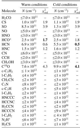
Table 5. Species column densities (in cm−2) in C2.
Warm conditions Cold conditions
Molecule N(cm−2) χ2red N(cm−2) χ2red
H2CO ≤7.0 × 10¹¹ – ≤7.0 × 10¹¹ − CS 1.0 × 10¹² 1.9 1.1 × 10¹² 1.9 SO 8.5 × 10¹¹ 3.9 1.3 × 10¹² 3.9 NO ≤5.0 × 10¹³ – ≤7.0 × 10¹³ – HNO ≤3.0 × 10¹¹ − ≤3.0 × 10¹¹ − HCO+ 2.5 × 10¹¹ 1.7 2.5 × 10¹¹ 1.8 HCN 6.9 × 10¹¹ 0.6 5.5 × 10¹¹ 0.5 HNC 1.5 × 10¹¹ 1.2 1.6 × 10¹¹ 1.2 CN ≤6.0 × 10¹² – ≤5.0 × 10¹² − CCH ≤2.0 × 10¹² – ≤2.0 × 10¹² – CH3OH ≤3.0 × 10¹² − ≤3.0 × 10¹² − C18O 7.6 × 10¹⁴ 4.3 9.9 × 10¹⁴ 4.1 c-C3H2 ≤ 1 × 10¹² − ≤1 × 10¹² − l-C3H2 ≤4 × 10¹⁰ − ≤1 × 10¹⁰ − CH3CN ≤2 × 10¹¹ − ≤3 × 10¹¹ − C3N ≤8 × 10¹² − ≤2 × 10¹³ − c-C3H ≤5 × 10¹² − ≤5 × 10¹² − l-C5H2 ≤2 × 10¹¹ − ≤1 × 10¹¹ − HNCCC ≤5 × 10¹¹ − ≤1 × 10¹² − HCCNC ≤2 × 10¹² − ≤4 × 10¹² − H2CCN ≤2 × 10¹⁰ − ≤2 × 1009 − HCCCN ≤4 × 10¹¹ − ≤9 × 10¹¹ − l-C4H2 ≤1 × 10¹¹ − ≤ 4 × 10¹⁰ − N2H+ ≤6 × 10¹¹ − ≤7 × 10¹¹ − H2CS ≤1 × 10¹² − ≤1 × 10¹² −
Notes. See Table3for the corresponding ‘warm’ and ‘cold’ conditions. Boldface indicates the smallest χ2 if both conditions do not give the same value. χ2
redstands for reduced χ2.
mean column density multiplied by a constant12CO/C18O ratio
of 557 (Wilson 1999). We assume here that there is no oxygen
isotopic fractionation based on Loison et al. (2019). We chose
CO as a reference because it was detected in all five sources. In addition, C18O is optically thin and so it is very likely to originate
from the same layer of material as the other molecules, which is
contrary to the properties of12CO and13CO. The CO abundance
can be affected by depletion but its abundance is less affected by other physical parameters, such as density and temperature.
For instance,Pratap et al.(1997) preferred to compare the
abun-dances with respect to HCO+. This molecule is less abundant
than CO and its abundance is more affected by the physical
conditions, as can be seen in Fig.D.1.
The abundances with respect to CO are shown in Fig. 4
for molecules detected in at least one of the clouds (listed in
Table A.1) and in Fig. 5 for the molecules detected in none
of the sources (listed in Table A.2). For comparison, we also
report the values from the literature for the cold clump TMC-1
(CP):Pratap et al.(1997) for HCO+, HCN, HNC, CN, CCH, and
N2H+;Gratier et al.(2016) for SO, CS, CH3OH, c-C3H2, l-C3H2,
CH3CN, C3N, c-C3H, HNCCC, HCCNC, H2CCN, HC3N,
l-C4H2, and H2CS;Ohishi & Kaifu(1998) for H2CO; andGerin
et al. (1993) for NO. As far as we know for this source, HNO
and l-C5H2 have not been reported in the literature. For CO,
the abundance reported by Pratap et al. (1997) is very high
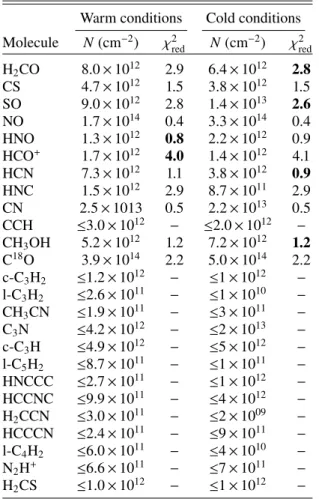
Table 6. Species column densities (in cm−2) in C3.
Warm conditions Cold conditions
Molecule N(cm−2) χ2red N(cm−2) χ2red
H2CO 8.0 × 10¹² 2.9 6.4 × 10¹² 2.8 CS 4.7 × 10¹² 1.5 3.8 × 10¹² 1.5 SO 9.0 × 10¹² 2.8 1.4 × 10¹³ 2.6 NO 1.7 × 10¹⁴ 0.4 3.3 × 10¹⁴ 0.4 HNO 1.3 × 10¹² 0.8 2.2 × 10¹² 0.9 HCO+ 1.7 × 10¹² 4.0 1.4 × 10¹² 4.1 HCN 7.3 × 10¹² 1.1 3.8 × 10¹² 0.9 HNC 1.5 × 10¹² 2.9 8.7 × 10¹¹ 2.9 CN 2.5 × 10¹³ 0.5 2.2 × 10¹³ 0.5 CCH ≤3.0 × 10¹² − ≤2.0 × 10¹² − CH3OH 5.2 × 10¹² 1.2 7.2 × 10¹² 1.2 C18O 3.9 × 10¹⁴ 2.2 5.0 × 10¹⁴ 2.2 c-C3H2 ≤1.2 × 10¹² − ≤1 × 10¹² − l-C3H2 ≤2.6 × 10¹¹ − ≤1 × 10¹⁰ − CH3CN ≤1.9 × 10¹¹ − ≤3 × 10¹¹ − C3N ≤4.2 × 10¹² − ≤2 × 10¹³ − c-C3H ≤4.9 × 10¹² − ≤5 × 10¹² − l-C5H2 ≤8.7 × 10¹¹ − ≤1 × 10¹¹ − HNCCC ≤2.7 × 10¹¹ − ≤1 × 10¹² − HCCNC ≤9.9 × 10¹¹ − ≤4 × 10¹² − H2CCN ≤3.0 × 10¹¹ − ≤2 × 1009 − HCCCN ≤2.4 × 10¹¹ − ≤9 × 10¹¹ − l-C4H2 ≤6.0 × 10¹¹ − ≤4 × 10¹⁰ − N2H+ ≤6.6 × 10¹¹ − ≤7 × 10¹¹ − H2CS ≤1.0 × 10¹² − ≤1 × 10¹² −
Notes. See Table3for the corresponding ‘warm’ and ‘cold’ conditions. Boldface indicates the smallest χ2 if both conditions do not give the same value. χ2
redstands for reduced χ2.
lower abundance of 8 × 10⁻⁵. A more recent study by Fuente
et al. (2019) obtained 9.7 × 10⁻⁵ from C18O observations. We
chose to use this last value to compute the species abundances with respect to CO in TMC-1, but the overall results are not sig-nificantly affected if alternative values are used. We note that
the H2column density used for the CO abundance is also
differ-ent from the other references (1.8 × 1022cm−2from Fuente et al.
2019, instead of the generally assumed value of 1022 cm−2), so
we scaled the abundance using the same H2 column densities
before dividing the species abundances.
Among our observed clouds, C3 presents clearly larger abundances with respect to CO while C2 seems to have smaller abundances. As compared to TMC-1 (CP), all our clumps have smaller abundances, except for the molecules CN, SO, CS, and NO; CN seems to be less abundant in TMC-1 (CP) than in
C1 and C3, while CH3OH and NO seem to be less abundant
in TMC-1 (CP) than in C3. Overall, all molecular abundances vary by nearly a factor of 10 or more from source to source. For the molecules that are not detected in any of our sources, half of them present an upper limit at the same level as the observed value in TMC-1 (CP) and half of them are below. As
an example, the upper limit on N2H+is not a strong constraint
while the HC3N upper limits are well below what is observed in
TMC-1 (CP).
Looking at the CS/SO abundance ratios in the different clumps, we find a small variation around 1: from 0.4 to 1.9.
Table 7. Species column densities (in cm−2) in C4.
Warm conditions Cold conditions
Molecule N(cm−2) χ2red N(cm−2) χ2red
H2CO 3.6 × 10¹² 1.7 3.7 × 10¹² 1.3 CS 7.3 × 10¹² 1.7 9.0 × 10¹² 1.7 SO 3.1 × 10¹² 1.6 5.9 × 10¹² 1.6 NO ≤5.0 × 10¹³ − ≤8.0 × 10¹³ − HNO ≤8.0 × 10¹¹ – ≤3.0 × 10¹¹ − HCO+ 5.9 × 10¹¹ 1.2 5.8 × 10¹¹ 1.2 HCN 7.3 × 10¹² 0.7 5.9 × 10¹² 0.6 HNC 8.6 × 10¹¹ 1.0 6.6 × 10¹¹ 0.9 CN ≤1.0 × 10¹³ − ≤1.0 × 10¹³ − CCH 6.6 × 10¹² 0.9 9.9 × 10¹² 0.9 CH3OH 2.4 × 10¹² 3.3 4.7 × 10¹² 3.2 C18O 1.5 × 10¹⁵ 6.2 2.2 × 10¹⁵ 5.5 c-C3H2 ≤8 × 10¹¹ − ≤6 × 10¹¹ − l-C3H2 ≤2 × 10¹¹ − ≤7 × 1009 − CH3CN ≤1 × 10¹¹ − ≤1 × 10¹¹ − C3N ≤2 × 10¹² − ≤9 × 10¹² − c-C3H ≤ 3 × 10¹² − ≤3 × 10¹² − l-C5H2 ≤4 × 10¹¹ − ≤5 × 10¹⁰ − HNCCC ≤1 × 10¹¹ − ≤5 × 10¹¹ − HCCNC ≤5 × 10¹¹ − ≤2 × 10¹² − H2CCN ≤2 × 10¹¹ − ≤9 × 1008 − HCCCN ≤1 × 10¹¹ − ≤4 × 10¹¹ − l-C4H2 ≤3 × 10¹¹ − ≤2 × 10¹⁰ − N2H+ ≤4 × 10¹¹ − ≤3 × 10¹¹ − H2CS ≤6 × 10¹¹ − ≤7 × 10¹² −
Notes. See Table3for the corresponding ‘warm’ and ‘cold’ conditions. Boldface indicates the smallest χ2 if both conditions do not give the same value. χ2
redstands for reduced χ2.
The ratio of HCN/HNC is always larger than 1: from 4 to 8.6. A ratio of HCN/HNC that is larger than one may indicate a non negligible abundance of atomic carbon in the gas phase as HNC is quickly converted to HCN through its reaction with C (Loison et al. 2014). NO/HNO is larger than 100 in C3 where both molecules were detected. The CN/NO abundance ratio is 0.1 in C3 and the HCN/CN ratio is 0.4 in C1 and 0.2 in C3. The
o/p ratio of H2CO is between 2.2 and 2.5 in all sources where it
was detected.
4. Chemical modelling
To chemically characterise the observed cores, we used the
gas-grain chemical code Nautilus (Ruaud et al. 2016). This model
follows the chemical evolution of the gas and ices surrounding interstellar grains by solving a set of differential equations. The various gas, gas-grain, and grain-surface processes included in
the model are described in Ruaud et al. (2016) while all the
chemical parameters are the ones described inWakelam et al.
(2019). For each source, we have run two models employing the
sets of physical conditions used to derive the observed column
densities (see Table3for the corresponding physical conditions).
We computed the chemistry for 107 yr starting from an atomic
composition (except for hydrogen, assumed to be entirely
molec-ular) with the same initial abundances as in Table 1 ofRuaud
et al.(2018). The elemental abundances for chemical models are the abundances of elements that remain in the gas-phase and
Table 8. Species column densities (in cm−2) in C5.
Warm conditions Cold conditions
Molecule N(cm−2) χ2red N(cm−2) χ2red
H2CO 2.8 × 10¹² 2.3 3.2 × 10¹² 2.3 CS 4.7 × 10¹² 0.9 5.9 × 10¹² 0.9 SO 3.1 × 10¹² 2 5.9 × 10¹² 1.8 NO ≤7.0 × 10¹³ – ≤9.0 × 10¹³ − HNO ≤4.0 × 10¹¹ − ≤4.0 × 10¹¹ − HCO+ 3.8 × 10¹¹ 1.1 4.7 × 10¹¹ 1.1 HCN 3.1 × 10¹² 0.5 2.5 × 10¹² 0.4 HNC 5.0 × 10¹¹ 0.7 5.0 × 10¹¹ 0.7 CN ≤7.0 × 10¹² − ≤8.0 × 10¹² − CCH ≤1.0 × 10¹² − ≤2.0 × 10¹² – CH3OH 2.2 × 10¹² 2.5 3.7 × 10¹² 2.4 C18O 5.0 × 10¹⁴ 2.8 7.6 × 10¹⁴ 2.8 c-C3H2 ≤9 × 10¹¹ − ≤1 × 10¹² − l-C3H2 ≤1 × 10¹¹ − ≤1 × 10¹⁰ − CH3CN ≤1 × 10¹¹ − ≤2 × 10¹¹ − C3N ≤4 × 10¹² − ≤1 × 10¹³ − c-C3H ≤3 × 10¹² − ≤4 × 10¹² − l-C5H2 ≤7 × 10¹¹ − ≤8 × 10¹⁰ − HNCCC ≤3 × 10¹¹ − ≤9 × 10¹¹ − HCCNC ≤1 × 10¹² − ≤3 × 10¹² − H2CCN ≤1 × 10¹¹ − ≤1 × 10⁹ − HCCCN ≤2 × 10¹¹ − ≤7 × 10¹¹ − l-C4H2 ≤4 × 10¹¹ − 3 ≤ × 1010 − N2H+ ≤5 × 10¹¹ − ≤6 × 10¹¹ − H2CS ≤8 × 10¹¹ − ≤1 × 10¹² −
Notes. See Table3for the corresponding ‘warm’ and ‘cold’ conditions. Boldface indicates the smallest χ2 if both conditions do not give the same value. χ2
redstands for reduced χ2.
H2CO CS SO NO HNO HCO+ HCN HNC CN CCH CH3OH 10 7 10 6 10 5 10 4 10 3 Abundance C1 C2 C3 C4 C5 TMC-1
Fig. 4.Species abundances (of the molecules listed in TableA.1) with respect to CO in each of the clouds. Arrows represent upper or lower limits. Vertical lines represent error bars computed from the variation of species column densities due to the uncertainty in the physical con-ditions. Blue points are the values reported in the literature towards the cold core TMC-1 (CP).
available for chemistry, while the rest are locked into refractory compounds. The choice of elemental abundances for the chem-ical modelling of cold cores is somewhat arbitrary as elemental depletion is observed to increase with the density in the diffuse medium but uncertainties remain on what happens for densities
larger than 10 cm−3 (conditions under which the atomic lines
c-C3H2 l-C3H2 CH3CN C3N c-C3H l-C5H2 HNCCC HCCNC H2CCN HCCCN l-C4H2 N2H+ H2CS 108 107 106 105 104 103 Abundance C1 C2 C3 C4 C5 TMC-1
Fig. 5.Upper limits on the species abundances not detected in any of the sources (and listed in TableA.2) with respect to CO in each of the clouds. Arrows represent upper or lower limits. Vertical lines represent error bars computed from the variation of species column densities due to the uncertainty in the physical conditions. Blue points are the values reported in the literature towards the cold core TMC-1 (CP).
cannot be observed any longer). So the constraints we have on these parameters are based on the observation of atomic abun-dances in the diffuse medium (that have also been reviewed over time with successive generations of telescopes). These observed abundances are very often modified to reduce the abundance of metals and sulphur. Many different values have been used in the literature, sometimes even tuned to reproduce one specific
obser-vation (see for instance discussions and references in Wakelam
& Herbst 2008;Wakelam et al. 2020). For this work, we used the abundances observed towards the diffuse region ζOph (v =
−15 km s−1) listed in Jenkins(2009) without additional
deple-tion, especially for sulphur, whose abundance is then fairly high compared to what is usually used for dense sources. For all sources, we assumed a standard’ cosmic-ray ionisation rate of
10−17s−1. We discuss the elemental abundances and the
cosmic-ray ionisation rate further in the remainder of this section. The visual extinction is taken to be 15 to limit the effect of direct UV photons as there is no indication that these are illuminated regions.
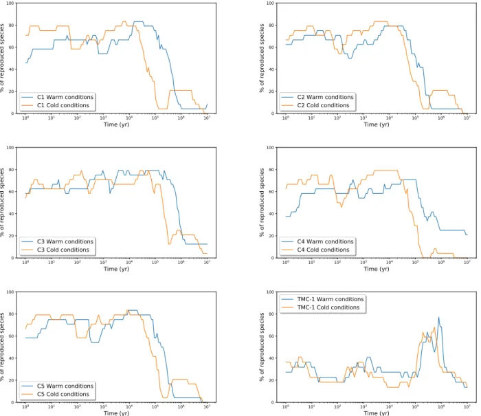
4.1. Comparing the model predictions with the observations From the observations, we have constraints on 24 species (not including CO). Among them, 5–11 are detected in our sources. To compare the model predictions with the observations, we
have followed the same approach as inWakelam et al.(2006) by
counting the number of species that are reproduced by our model at each time. We assume an agreement if a species is detected and its abundance is within a factor of 10 of the modelled abundance. If the species is not detected, we have an upper limit. In that case, we assume that the modelled abundance has to be below the observed upper limit. Since the factor of 10 is an approxi-mate uncertainty, we assume that the observed upper limit needs to be larger than the modelled abundance divided by 10 (mean-ing that the ratio between the modelled and observed upper limit needs to be smaller than 10). If we had chosen a more conser-vative approach, assuming for instance that the observed upper limit has to be larger than ten times the modelled abundance, then our agreement between modelled and observed abundances would be less than the results shown in this section. These indi-cators of agreement need to be taken with caution and are not a
100 101 102 103 104 105 106 107 Time (yr) 0 20 40 60 80 100 % of reproduced species C1 Warm conditions C1 Cold conditions 100 101 102 103 104 105 106 107 Time (yr) 0 20 40 60 80 100 % of reproduced species C2 Warm conditions C2 Cold conditions 100 101 102 103 104 105 106 107 Time (yr) 0 20 40 60 80 100 % of reproduced species C3 Warm conditions C3 Cold conditions 100 101 102 103 104 105 106 107 Time (yr) 0 20 40 60 80 100 % of reproduced species C4 Warm conditions C4 Cold conditions 100 101 102 103 104 105 106 107 Time (yr) 0 20 40 60 80 100 % of reproduced species C5 Warm conditions C5 Cold conditions 100 101 102 103 104 105 106 107 Time (yr) 0 20 40 60 80 100 % of reproduced species TMC-1 Warm conditions TMC-1 Cold conditions
Fig. 6.Percentage of species reproduced by the different models for each source as a function of time. ‘Warm’ conditions and ‘cold’ conditions refer to the set of physical conditions as listed in Table3.
real indication of quality of model but are, rather, used to com-pare one model with the other. For TMC-1, we have two lower limits (due to optical depth effects); thus, for these points to get an agreement, the observed lower limit needs to be smaller than the modelled abundance multiplied by ten. If these cri-teria are not fulfilled, then we do not have agreement. Since
we do not have any estimate on the H2 column densities, we
again use CO as a reference and compare the observed and mod-elled species abundances with respect to CO. We also ran two models for TMC-1 using the physical conditions determined by
Lique et al. (2006) (a temperature of 8 K for a H2 density of
3 × 104cm−3) and byFuente et al.(2019) (10 K for a H
2density
of 1.5 × 104cm−3). These conditions are very similar to what we
found in our sample.
Figure6shows the percentage of reproduced species in each
source for each model (see Table3for a summary of the
physi-cal conditions). Overall, we find a good agreement, with between 79 and 83% of the molecules reproduced by the models. For TMC-1, the agreement is still good (68–77%). The percentage of reproduced species might seem smaller than for our sources, however, it is important to keep in mind that in TMC-1, all con-sidered molecules are detected while in our sources, we mostly
have upper limits, which makes the comparison with the model
less robust. In Table9, we report some constraints (best
percent-age and time) derived from the model/observation comparison. For each source, we have two different physical conditions. The last column of the table lists the species that are not reproduced by the model at the ‘best time’. A graphic view of the model
agreement is shown in AppendixF. In Figs.F.1andF.2, we show
for each model the ratio between the modelled and observed abundances at the best times.
The first obvious result is that the strongest constraints on the time are upper limits as the agreement for all sources drops
sharply after a few 104or 105yr, depending on the source. The
maximum time is higher for lower-density models. Indeed, the model needs more time to achieve a similar chemical stage if the density is lower. Here, C4 is the only source for which one of the two sets of physical conditions (the ‘cold’ ones) seems to better agree with the observations. Both physical conditions for TMC-1 seem to indicate a more evolved source, which is in agreement with the fact that a lot of molecules are detected (and these are more abundant) in this source as opposed to the other ones.
Looking at the species that are not reproduced by the models at the best times in C1 to C5 sources, most of them are among
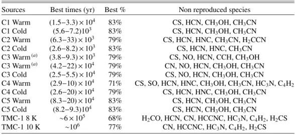
Table 9. Percentage of species reproduced by the models in each source, corresponding best times and species not reproduced.
Sources Best times (yr) Best % Non reproduced species
C1 Warm (1.5−3.3) × 104 83% CS, HCN, CH 3OH, CH3CN C1 Cold (5.6−7.2)103 83% CS, HCN, CH3OH, CH3CN C2 Warm (6.3−33) × 103 79% CS, HCN, HNC, CH 3CN, H2CCN C2 Cold (2.6−8.2) × 103 83% CS, HCN, HNC, CH 3CN
C3 Warm(a) (3.8−9.3) × 103 79% CS, NO, HCN, CCH, CH3OH
C3 Warm(a) (4.2−22) × 104 79% CN, NO, HCN, CH
3OH, CH3CN
C3 Cold (2.5−5.5) × 104 79% CS, NO, HCN, CH
3OH, CH3CN
C4 Warm (2.9−10) × 104 71% CS, SO, HCN, HNC, CH3OH, CH3CN, HC3N, C4H2
C4 Cold (2.6−20) × 104 79% CS, HCN, HNC, CH 3OH, CH3CN C5 Warm (8.3−20) × 104 83% CS, HCN, CH 3OH, CH3CN C5 Cold (8.2−9.3)104 83% CS, HCN, CH3OH, CH3CN TMC-1 8 K ∼6 × 10⁵ 68% H 2CO, HCN, CN, HCCNC, HC3N, C4H2, H2CS TMC-1 10 K ∼106 77% CN, HCCNC, HC3N, C4H2, H2CS
Notes. See text for details. ‘Warm’ and ‘cold’ refer to the set of physical conditions as listed in Table3. C3 Warmaandbare two different periods of time giving the same agreement.(a)There are two different periods of time giving the same agreement for C3.
the detected ones (in particular, CS, HCN, and CH3OH), which
weakens our analysis. The smaller times that we obtain (as com-pared to TMC-1) can be explained by the fact that molecules will build up with time slower than CO. They reach a maximum at times when CO has already started to deplete. So the model can only reproduce the small observed abundances (and the non-detections) at early times. For CS and HCN, whatever the time, the model overestimates the abundance. The fact that chemical models overestimate the CS abundance in cold cores has also
been found in previous studies (Navarro-Almaida et al. 2020).
The possible failure of the model for this molecule will be
dis-cussed inBulut et al.(2021). For HCN, this may indicate that our
observed abundance is underestimated. In fact, in our observa-tions, the ratio between the three hyperfine lines of the 1–0 HCN line is not 1:5:3, as expected from the line parameters, but 2:5:3
(Fig.3). Anomalies in the HCN hyperfine structures are frequent
in cold cores and their origin has been the subject of several stud-ies (Guilloteau & Baudry 1981;Gonzalez-Alfonso & Cernicharo
1993). Among the causes, optical depth effects, overlap effects of
2–1 hyperfine transition to the 1–0 hyperfine intensity ratio, and the density and velocity structures of cold cores have been found to affect this ratio. All these effects would not necessarily affect the overall derived abundance, except for optical depth effects. Beam dilution may on the contrary produce an underestimation of the real abundance if the emitting structure were smaller than our beam. These could also explain the very low temperatures found from the radiative transfer analysis of the 1–0 HCN line. In addition, CS is reproduced in the TMC-1 model because the observations only give a lower limit due to opacity effects. 4.2. Effect of the cosmic-ray ionisation rate and elemental
abundances
For the simulations presented above, we have considered a ‘stan-dard’ cosmic-ray ionisation rate of 10−17s−1(Solomon & Werner
1971). This value is highly uncertain. In TMC-1, Nejad et al.
(1994) estimated ζ to be between 3 × 10⁻¹⁷s−1and 8 × 10⁻¹⁷s−1
while Pratap et al.(1997) found a ζ of 6 × 10⁻¹⁷ s−1. We used
this later value and ran all the models presented in the previous section once again. The comparison between these new models
and the observations are presented in Fig.E.1. The results are
not significantly different and the list of species not
repro-duced given in Table9stands. The only real change is that the
TMC-1 observations are better reproduced by the colder and denser model.
Another model parameter that is not well constrained is the elemental abundances. Atoms are known to deplete in the dif-fuse interstellar medium, a depletion that is not fully understood
or quantified at this stage (Tielens 1998;Whittet 2010;Jenkins
2009). As the initial conditions for our models, we chose to
use the atomic abundances observed in the diffuse medium, while many chemical studies assume more depleted values that
are usually refereed as ‘low metal’ conditions (Graedel et al.
1982). Among the elements, sulphur is probably the one whose
elemental abundance is the most varied in models in order to reproduce the low observed abundances of S-bearing species in
cold sources (see for instance Vidal et al. 2017). In our
previ-ous models, we have used the cosmic abundance of sulphur as its elemental abundance. To test the effect of this parameter, we have run the same models with a ten times smaller abundance
(i.e. 3 × 10⁻⁶with respect to H2). The comparison of these
mod-els with the observations is shown in Fig.E.2. Overall, the results are not much changed. The agreement is similar or slightly worse with our sources. SO and CS are not better reproduced. The com-parison with TMC-1 is slightly better but the best times do not change.
The C/O elemental ratio is very often varied (from smaller than 1 to larger than 1) to reproduce the large abundances of
carbon bearing species (Herbst & Leung 1986; Bettens et al.
1995; Hincelin et al. 2011). We tested the effect of increasing this ratio to 1.2 by decreasing the oxygen elemental abundance. As expected, the observations in TMC-1 are better reproduced
(see Fig.E.3) at times between 1 × 10⁵and 4 × 10⁵yr with both
physical conditions. The agreement is less good for the other sources.
5. Conclusion
In this work, we observe two large spectral bands (71–116 GHz and 126–182 GHz) in five cold clumps of the Planck Early Core catalogue, located in three different large molecular clouds (California, Perseus, and Taurus molecular clouds). Within these
sources, only a small number of molecules were detected (H2CO,
CS, SO, NO, HNO, HCO+, HCN, HNC, CN, CCH, CH
3OH, and
CO), as compared to the long list of targeted molecules seen in cold cores such as TMC-1(CP). A study of the excitation con-ditions of molecules such as CO, HCN, SO, and CS has shown incompatibilities: HCN (1–0) observed lines can only be
repro-duced by very low temperature (of 5 K) while the 12CO and
13CO (1–0) lines indicate higher temperatures and lower
densi-ties. The12CO and13CO (1–0) lines are optically thick, contrary
to the other observed lines. The12CO and13CO (1–0) lines very
likely originate from the external warmer and less dense layers of the clumps while the other lines probe inner denser and colder regions. In addition, there may have some substructures within the antenna beam that could explain why we have systematically
larger CO fluxes as compared toMeng et al.(2013), who mapped
the region with a larger beam.
Based on two different assumed physical conditions (one constrained by HCN and the other constrained by CS and CO), we computed the species column densities. Overall, the com-puted column densities are not very sensitive to the assumed physical conditions. Assuming that the CO abundance
(com-puted from optically thin C18O) is the same in all sources (which
may not be the case), the molecular abundances are spread over almost one order of magnitude in the different sources. Com-pared to TMC-1(CP), these clumps appear quite poor both in abundance levels and in molecular diversity. We did not detect any carbon chain molecules.
With a full gas-grain model and the physical conditions derived in each source, we are able to reproduce between 79% and 83% of the observed species (including the upper limits). This is slightly better than in TMC-1, we note, however: (1) we do not reproduce CS and HCN, which are both overestimated by the models; and (2) we have mostly upper limits, a condition that provides fewer constraints for the model. The ‘best’ times for our sources seem to be smaller than for TMC-1, indicating that our sources may be less evolved; this allows us to explain the smaller abundances and the numerous non-detections. Consider-ing a cosmic-ray ionisation rate that is larger than the standard
10−17 s−1 one does not significantly impact our results. If we
deplete the sulphur as compared to cosmic values the agree-ment between the model and the CS observed abundance is not improved. If we increase the C/O elemental ratio, we improve the model agreement with TMC-1, but worsening it for the sources presented here.
Acknowledgements. The authors acknowledge the CNRS program “Physique
et Chimie du Milieu Interstellaire” (PCMI) co-funded by the Centre National d’Etudes Spatiales (CNES). M.R. research was supported by an appointment to the NASA Postdoctoral Program at NASA Ames Research Center, administered by Universities Space Research Association under contract with NASA.
References
Agúndez, M., & Wakelam, V. 2013,Chem. Rev., 113, 8710
Bacmann, A., Taquet, V., Faure, A., Kahane, C., & Ceccarelli, C. 2012,A&A,
541, L12
Bergin, E. A., & Tafalla, M. 2007,ARA&A, 45, 339
Bettens, R. P. A., Lee, H. H., & Herbst, E. 1995,ApJ, 443, 664
Bulut, N., Roncero, O., Aguado, A., et al. 2021,A&A, 646, A5
Cernicharo, J., Marcelino, N., Roueff, E., et al. 2012,ApJ, 759, L43
Crutcher, R. M., Churchwell, E., & Ziurys, L. M. 1984,ApJ, 283, 668
Dame, T. M., Ungerechts, H., Cohen, R. S., et al. 1987,ApJ, 322, 706
Denis-Alpizar, O., Stoecklin, T., Halvick, P., & Dubernet, M.-L. 2013, J. Chem. Phys., 139, 204304
Denis-Alpizar, O., Stoecklin, T., Guilloteau, S., & Dutrey, A. 2018,MNRAS,
478, 1811
Dickens, J. E., Irvine, W. M., Snell, R. L., et al. 2000,ApJ, 542, 870
Dumouchel, F., Kłos, J., & Lique, F. 2011,Phys. Chem. Chem. Phys., 13, 8204
Fuente, A., Navarro, D. G., Caselli, P., et al. 2019,A&A, 624, A105
Gerin, M., Viala, Y., & Casoli, F. 1993,A&A, 268, 212
Gonzalez-Alfonso, E., & Cernicharo, J. 1993,A&A, 279, 506
Graedel, T. E., Langer, W. D., & Frerking, M. A. 1982,ApJS, 48, 321
Gratier, P., Majumdar, L., Ohishi, M., et al. 2016,ApJS, 225, 25
Guilloteau, S., & Baudry, A. 1981,A&A, 97, 213
Herbst, E., & Leung, C. M. 1986,MNRAS, 222, 689
Hernández Vera, M., Lique, F., Dumouchel, F., Hily-Blant, P., & Faure, A. 2017, MNRAS, 468, 1084
Hincelin, U., Wakelam, V., Hersant, F., et al. 2011,A&A, 530, A61
Jenkins, E. B. 2009,ApJ, 700, 1299
Kalugina, Y., Lique, F., & Kłos, J. 2012,MNRAS, 422, 812
Lada, C. J., Lombardi, M., & Alves, J. F. 2009,ApJ, 703, 52
Lique, F., Cernicharo, J., & Cox, P. 2006,ApJ, 653, 1342
Lique, F., Senent, M.-L., Spielfiedel, A., & Feautrier, N. 2007,J. Chem. Phys.,
126, 164312
Lique, F., van der Tak, F. F. S., Kłos, J., Bulthuis, J., & Alexander, M. H. 2009, A&A, 493, 557
Liu, X.-C., Wu, Y., Zhang, C., et al. 2019,A&A, 622, A32
Loison, J.-C., Wakelam, V., & Hickson, K. M. 2014,MNRAS, 443, 398
Loison, J.-C., Wakelam, V., Gratier, P., et al. 2019,MNRAS, 485, 5777
Lombardi, M., Lada, C. J., & Alves, J. 2010,A&A, 512, A67
Meng, F., Wu, Y., & Liu, T. 2013,ApJS, 209, 37
Müller, H. S. P., Schlöder, F., Stutzki, J., & Winnewisser, G. 2005,J. Mol. Struc.,
742, 215
Navarro-Almaida, D., Le Gal, R., Fuente, A., et al. 2020,A&A, 637, A39
Nejad, L. A. M., Hartquist, T. W., & Williams, D. A. 1994,Ap&SS, 220, 261
Ohishi, M., & Kaifu, N. 1998,Faraday Discuss., 109, 205
Ohishi, M., Irvine, W. M., & Kaifu, N. 1992,IAU Symp., 150, 171
Padovani, M., Walmsley, C. M., Tafalla, M., Hily-Blant, P., & Pineau Des Forêts,
G. 2011,A&A, 534, A77
Pagani, L., Bacmann, A., Motte, F., et al. 2004,A&A, 417, 605
Pety, J. 2005, in SF2A-2005: Semaine de l’Astrophysique Française, eds.
F. Casoli, T. Contini, J. M. Hameury, & L. Pagani (France: EDP-Sciences), 721
Planck Collaboration XXII. 2011,A&A, 536, A22
Planck Collaboration XXVIII. 2016,A&A, 594, A28
Pratap, P., Dickens, J. E., Snell, R. L., et al. 1997,ApJ, 486, 862
Quénard, D., Vastel, C., Ceccarelli, C., et al. 2017,MNRAS, 470, 3194
Rabli, D., & Flower, D. R. 2010,MNRAS, 406, 95
Ruaud, M., Wakelam, V., & Hersant, F. 2016,MNRAS, 459, 3756
Ruaud, M., Wakelam, V., Gratier, P., & Bonnell, I. A. 2018,A&A, 611, A96
Solomon, P. M., & Werner, M. W. 1971,ApJ, 165, 41
Spielfiedel, A., Feautrier, N., Najar, F., et al. 2012,MNRAS, 421, 1891
Tielens, A. G. G. M. 1998,ApJ, 499, 267
van der Tak, F. F. S., Black, J. H., Schöier, F. L., Jansen, D. J., & van Dishoeck,
E. F. 2007,A&A, 468, 627
Vastel, C., Ceccarelli, C., Lefloch, B., & Bachiller, R. 2014,ApJ, 795, L2
Vidal, T. H. G., Loison, J.-C., Jaziri, A. Y., et al. 2017,MNRAS, 469, 435
Wakelam, V., & Herbst, E. 2008,ApJ, 680, 371
Wakelam, V., Herbst, E., & Selsis, F. 2006,A&A, 451, 551
Wakelam, V., Smith, I. W. M., Herbst, E., et al. 2010,Space Sci. Rev., 156, 13
Wakelam, V., Ruaud, M., Gratier, P., & Bonnell, I. A. 2019,MNRAS, 486,
4198
Wakelam, V., Iqbal, W., Melisse, J. P., et al. 2020,MNRAS, 497, 2309
Whittet, D. C. B. 2010,ApJ, 710, 1009
Wiesenfeld, L., & Faure, A. 2013,MNRAS, 432, 2573
Wilson, T. L. 1999,Rep. Prog. Phys., 62, 143
Wu, Y., Liu, T., Meng, F., et al. 2012,ApJ, 756, 76
Yang, B., Stancil, P. C., Balakrishnan, N., & Forrey, R. C. 2010,ApJ, 718, 1062
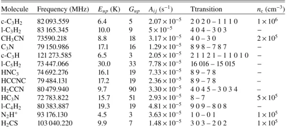
Appendix A: Line properties in the five sources
Table A.1. Detected transitions.
Molecule Frequency (MHz) Eup(K) Gup Ai j(s−1) Transition nc(cm−3)
H2CO 72 837.948 3.5 3 8.15e-06 1 0 1 – 0 0 0 2 × 10⁵ H2CO 140 839.502 21.9 15 5.30e-05 2 1 2 – 1 1 1 7 × 10⁵ H2CO 145 602.949 10.5 5 7.81e-05 2 0 2 – 1 0 1 8 × 10⁵ H2CO 150 498.334 22.6 15 6.47e-05 2 1 1 – 1 1 0 1 × 10⁶ CS 97 980.950 7.1 5 1.69e-05 2 – 1 4 × 10⁵ CS 146 969.033 14.1 7 6.11e-05 3 – 2 1 × 10⁶ C34S 96 412.940 6.9 5 1.61e-05 2 – 1 − SO 99 299.870 9.2 7 1.15e-05 2 3 – 1 2 2 × 10⁵ SO 138 178.600 15.9 9 3.23e-05 3 4 – 2 3 4 × 10⁵ NO 150 176.480 7.2 6 3.31e-07 2-1 2 3 – 1 1 1 2 2 × 10⁴ NO 150 198.760 7.2 4 1.84e-07 2-1 2 2 – 1 1 1 1 2 × 10⁴ NO 150 218.730 7.2 4 1.47e-07 2-1 2 2 – 1 1 1 2 1 × 10⁴ NO 150 225.660 7.2 2 2.94e-07 2-1 2 1 – 1 1 1 1 4 × 10⁴ NO 150 439.120 7.2 4 1.48e-07 2 1 2 2 – 1-1 1 2 1 × 10⁴ NO 150 546.520 7.2 6 3.33e-07 2 1 2 3 – 1-1 1 2 2 × 10⁴ NO 150 580.560 7.2 2 2.96e-07 2 1 2 1 – 1-1 1 1 4 × 10⁴ NO 150 644.340 7.2 4 1.85e-07 2 1 2 2 – 1-1 1 1 2 × 10⁴ HNO 81 477.490 3.9 5 2.23e-06 1 0 1 2 – 0 0 0 1 − HNO 81 477.490 3.9 3 2.23e-06 1 0 1 1 – 0 0 0 1 − HNO 81 477.490 3.9 1 2.23e-06 1 0 1 0 – 0 0 0 1 − HCO+ 89 188.523 4.3 3 4.16e-05 1 0 0 – 0 0 0 2 × 10⁵ HCO+ 178 375.010 12.8 5 4.00e-04 2 0 0 – 1 0 0 9 × 10⁵ H13CO+ 86 754.288 4.2 3 3.83e-05 1 – 0 − HCN 88 630.416 4.3 3 2.43e-05 1 1 – 0 1 1 × 10⁶ HCN 88 631.847 4.3 5 2.43e-05 1 2 – 0 1 1 × 10⁶ HCN 88 633.936 4.3 1 2.43e-05 1 0 – 0 1 1 × 10⁶ HNC 90 663.593 4.4 3 2.69e-05 1 – 0 3 × 10⁵ CN 113 144.190 5.4 2 1.05e-05 1 1 2 1 2 – 0 1 2 3 2 2 × 10⁶ CN 113 191.325 5.4 4 6.68e-06 1 1 2 1 2 – 0 3 2 3 2 3 × 10⁶ CN 113 488.142 5.4 4 6.73e-06 1 3 2 1 2 – 0 3 2 1 2 3 × 10⁶ CN 113 490.985 5.4 6 1.19e-05 1 3 2 1 2 – 0 5 2 3 2 3 × 10⁶ CCH 87 316.925 4.2 5 1.65e-06 1 2 2 – 0 1 1 1 × 10⁵ CCH 87 402.004 4.2 3 1.38e-06 1 1 1 – 0 1 1 1 × 10⁵ CH3OH 96 739.358 12.5 5 2.56e-06 2-1 0 – 1-1 0 3 × 10⁴ CH3OH 96 741.371 7.0 5 3.41e-06 2 0 + 0 – 1 0 + 0 3 × 10⁴ CH3OH 145 097.435 19.5 7 1.10e-05 3-1 0 – 2-1 0 3 × 10⁵ CH3OH 145 103.185 13.9 7 1.23e-05 3 0 + 0 – 2 0 + 0 1 × 10⁵ C18O 109 782.173 5.3 3 6.27e-08 1 – 0 2 × 10³ 13CO 110 201.354 5.3 3 6.33e-08 1 – 0 2 × 10³ C17O(a) 112 359.284 5.4 3 6.70e-08 1 – 0 2 × 10³ CO 115 271.202 5.5 3 7.20e-08 1 – 0 2 × 10³
Notes. (a)C17O has a hyperfine structure with three lines at 112 358.7770, 112 358.9820, and 112 360.0070 MHz according to the CMDS database. Both the JPL and LAMDA databases (which our CASSIS analysis is based on) assume only one component at 112 359.284 MHz. In our observations, the lines at 112 358.7770 MHz and 112 358.9820 MHz are blended.
Table A.2. Transitions used to determine upper limit for molecules detected in none of the sources.
Molecule Frequency (MHz) Eup(K) Gup Ai j(s−1) Ttransition nc(cm−3)
c-C3H2 82 093.559 6.4 5 2.07 × 10⁻⁵ 2 0 2 0 – 1 1 1 0 1 × 10⁶ l-C3H2 83 165.345 10.0 9 5 × 10⁻⁵ 4 0 4 – 3 0 3 − CH3CN 73590.218 8.8 18 3.17 × 10⁻⁵ 4 0 – 3 0 2 × 10⁵ C3N 79 150.986 17.1 16 1.29 × 10⁻⁵ 8 9 8 – 7 8 7 − c-C3H 121 273.585 6.5 3 2.05 × 10⁻⁵ 2 1 1 2 1 – 1 1 0 1 0 − l-C5H2 73 447.066 30.0 33 7.78 × 10⁻⁵ 16 016 – 15 015 − HNC3 74 692.276 16.1 19 7.33 × 10⁻⁵ 8 9 – 7 8 − HCCNC 79 484.131 17.2 19 2.36 × 10⁻⁵ 8 9 – 7 8 – H2CCN 80 479.940 9.7 90 3.30 × 10⁻⁵ 4 0 4 5 – 3 0 3 4 – HC3N 72 783.822 15.7 51 2.93 × 10⁻⁵ 8 – 7 5 × 10⁵ l-C4H2 80 383.887 19.3 19 4.81 × 10⁻⁵ 9 0 9 – 8 0 8 − N2H+ 93 176.130 4.5 3 3.63 × 10⁻⁵ 1 0 – 0 1 1 × 10⁵ H2CS 103 040.220 9.9 7 1.48 × 10⁻⁵ 3 0 3 – 2 0 2 1 × 10⁵
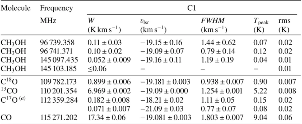
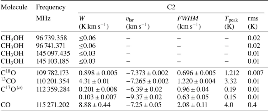
Table A.3. Results of line fitting in C1.
Molecule Frequency C1 MHz W vlsr FWHM Tpeak rms (K km s−1) (km s−1) (km s−1) (K) (K) H2CO 72 837.948 0.35 ± 0.02 −19.04 ± 0.03 1.09 ± 0.06 0.30 0.02 H2CO 140 839.502 0.24 ± 0.09 −19.22 ± 0.02 0.99 ± 0.04 0.22 0.01 H2CO 145 602.949 0.08 ± 0.02 −19.29 ± 0.08 0.75 ± 0.23 0.10 0.02 H2CO 150 498.334 0.13 ± 0.01 −19.04 ± 0.04 1.14 ± 0.09 0.10 0.01 CS 97 980.950 0.59 ± 0.01 −19.08 ± 0.01 1.16 ± 0.03 0.48 0.02 CS 146 969.033 0.19 ± 0.01 −19.04 ± 0.03 1.05 ± 0.06 0.17 0.01 C34S 96 412.940 ≤0.06 − – − 0.01 SO 99 299.870 0.54 ± 0.01 −19.15 ± 0.01 0.99 ± 0.02 0.51 0.01 SO 138 178.600 0.18 ± 0.01 −19.23 ± 0.03 0.86 ± 0.06 0.19 0.01 NO 150 176.480 ≤0.06 − – − 0.01 NO 150 198.760 ≤0.06 − – − 0.01 NO 150 218.730 ≤0.06 − – − 0.01 NO 150 225.660 ≤0.06 − – − 0.01 NO 150 439.120 ≤0.06 − – − 0.01 NO 150 546.520 ≤0.06 − – − 0.01 NO 150 580.560 ≤0.06 − – − 0.01 NO 150 644.340 ≤0.06 − – − 0.01 HNO 81 477.490 ≤0.02 − – − 0.007 HCO+ 89 188.523 0.66 ± 0.01 −19.23 ± 0.01 1.29 ± 0.02 0.48 0.01 HCO+ 178 375.010 0.27 ± 0.03 −19.30 ± 0.07 1.34 ± 0.21 0.19 0.04 H13CO+ 86 754.288 ≤0.06 − – − 0.01 HCN 88 630.416 0.177 ± 0.007 −19.08 ± 0.02 1.12 ± 0.04 0.15 0.007 HCN 88 631.847 0.298 ± 0.007 −19.09 ± 0.06 1.24 ± 0.03 0.22 0.007 HCN 88 633.936 0.119 ± 0.007 −19.01 ± 0.22 1.22 ± 0.08 0.09 0.007 HNC 90 663.593 0.23 ± 0.01 −18.96 ± 0.03 1.39 ± 0.08 0.16 0.01 CN 113 144.190 ≤0.06 − – − 0.01 CN 113 191.325 ≤0.06 − – − 0.01 CN 113 488.142 ≤0.06 − – − 0.01 CN 113 490.985 0.06 ± 0.01 −18.98 ± 0.05 0.76 ± 0.12 0.07 0.01 CCH 87 316.925 0.05 ± 0.01 −18.56 ± 0.11 1.06 ± 0.22 0.04 0.01 CCH 87 402.004 ≤0.06 − – − 0.01
Notes. (a)C17O has a hyperfine structure; see comment in TableA.1. W is the integrated intensity, v
lsrthe central velocity, FWHM the line width, and Tpeakthe peak intensity of a Gaussian fitting of each line. The rms is the noise level of each line.