HAL Id: hal-00303044
https://hal.archives-ouvertes.fr/hal-00303044
Submitted on 21 Oct 2004
HAL is a multi-disciplinary open access
archive for the deposit and dissemination of
sci-entific research documents, whether they are
pub-lished or not. The documents may come from
teaching and research institutions in France or
abroad, or from public or private research centers.
L’archive ouverte pluridisciplinaire HAL, est
destinée au dépôt et à la diffusion de documents
scientifiques de niveau recherche, publiés ou non,
émanant des établissements d’enseignement et de
recherche français ou étrangers, des laboratoires
publics ou privés.
Characterization of Strombolian events by using
independent component analysis
A. Ciaramella, E. de Lauro, S. de Martino, B. Di Lieto, M. Falanga, R.
Tagliaferri
To cite this version:
A. Ciaramella, E. de Lauro, S. de Martino, B. Di Lieto, M. Falanga, et al.. Characterization of
Strombolian events by using independent component analysis. Nonlinear Processes in Geophysics,
European Geosciences Union (EGU), 2004, 11 (4), pp.453-461. �hal-00303044�
SRef-ID: 1607-7946/npg/2004-11-453
Nonlinear Processes
in Geophysics
© European Geosciences Union 2004
Characterization of Strombolian events by using independent
component analysis
A. Ciaramella1, E. De Lauro2, S. De Martino2, 3, 4, B. Di Lieto2, M. Falanga2, 3, 4, and R. Tagliaferri1
1Dipartimento di Matematica ed Informatica, Salerno University, via S. Allende, I-84081 Baronissi (SA), Italy
2Dipartimento di Fisica, Salerno University, via S. Allende, I-84081 Baronissi (SA), Italy
3INFM, unit`a di Salerno, via S. Allende, I-84081 Baronissi (SA), Italy
4INFN, gruppo collegato di Salerno, via S. Allende, I-84081 Baronissi (SA), Italy
Received: 16 June 2004 – Revised: 13 October 2004 – Accepted: 14 October 2004 – Published: 21 October 2004 Part of Special Issue “Nonlinear analysis of multivariate geoscientific data – advanced methods, theory and application”
Abstract. We apply Independent Component Analysis (ICA) to seismic signals recorded at Stromboli volcano. Firstly, we show how ICA works considering synthetic sig-nals, which are generated by dynamical systems. We prove that Strombolian signals, both tremor and explosions, in the high frequency band (>0.5 Hz), are similar in time domain. This seems to give some insights to the organ pipe model generation for the source of these events. Moreover, we are able to recognize in the tremor signals a low frequency com-ponent (<0.5 Hz), with a well defined peak corresponding to 30 s.
1 Introduction
The classical procedure to construct physical models is sim-ple and well established. Firstly, rough but explanatory mo-dels are inferred from phenomenology. At this preliminary stage, many possible intuitive pictures live together. They are used to reproduce, on laboratory scale, all the relevant observational aspects. The experiments are, in general, re-producible and some physical laws can be established. These seminal models are improved and discriminated according to their capability to provide new phenomena to test expe-rimentally. There are, however, physical systems for which it is impossible to proceed in this way. In fact, even simple phenomenological aspects cannot be reproduced on labora-tory scale, both for practical and conceptual reasons. These systems are characterized by strong nonlinear behaviour that involves many time and spatial length scales.
Geophysical systems belong to this class. In this and simi-lar cases, people speak about observational data rather than experimental data. Sequences, signals, messages, texts, con-figurations are examples of observational data. Among them, Correspondence to: M. Falanga
an important role is played by the observations (measure-ments) made in the course of the time, i.e. scalar time series. We can associate, in a natural way, the concepts of complexi-ty, statistics, ergodicity to these series in order to distinguish them, quantitatively. All the sequences can be described, in a formal way, by the unifying concept of Dynamical System (DS). Many theorems and mathematical devices have been elaborated to study DSs. However, they give powerful me-thods to study asymptotic properties. In the real experimental cases, we start from finite sequences, sometimes very long, and we want to obtain the model. The problem is to extract relevant properties from one or more of the available scalar finite sequences. Then, numerical analysis arises to under-stand all important parts of information included within se-ries. A review of many numerical methods of nonlinear sig-nal processing developed in the recent years can be found in Abarbanel (1996).
In many cases, sequences can contain information relative to different DSs or sources or signals: therefore a preliminary step is to recognize independent components. The methods based on information theory are natural to use in this research field. The concept of entropy plays a particular role: it is very general and gives a powerful methodology to distinguish the complexities associated to different DSs.
Independent Component Analysis (ICA) is an entropy based technique, useful to separate mixtures of signals (for more details see Hyv¨arinen et al. (2001) and many papers therein cited). ICA was introduced in the early 1980s in a neurophysiological setting (H´erault, 1984). The introduction of FastICA algorithm (Hyv¨arinen and Oja, 1997) contributed to the application of ICA to large scale problems due to its computational efficiency.
In the next section, we shall give the mathematical set-ting of ICA. Here, we consider the problem to understand the behaviour of ICA method with respect to scalar time se-ries generated by geophysical systems. Since they can be
454 A. Ciaramella et al.: Strombolian events and ICA interpreted as time evolution of a suitable dynamical system,
we start clarifying the performance of ICA when it is applied to known DSs. We select different DSs equations representa-tive of large classes, namely linear, nonlinear in the regime of limit cycle, and stochastic DSs, and we use ICA to make sep-aration of the generated synthetic signals. After this section, we show the application of ICA to observational recorded time series of Stromboli volcano.
2 Independent component analysis
ICA is a method to find underlying factors or components from multivariate (multidimensional) statistical data.
It is a well defined method in speech context, to solve the classical problem of cocktail party. Imagine to have some people speaking in a room and some microphones recording their voice. The goal of ICA is to extract, from the mixtures of voices, step by step, each independent speaker.
Let us explain in brief the mathematical setting on which ICA is based. We can suppose to have m different recorded time series x, that we hypothesize to be the linear superpo-sition of n mutually independent unknown sources s, due to different mixing, represented by a constant unknown m × n
matrix A. This mixing is essentially due to path, noise,
instrumental transfer-functions, etc. The hypothesis is to have instantaneous linear mixtures of some independent dy-namical systems. If the mixing has to be linear, nothing is assumed with respect to the sources, which can be linear or nonlinear.
Formally, the mixing model is written as
x = As + µ. (1)
The term µ takes into account the presence of an additive noise, often omitted in Eq. (1), because it can be incorporated in the sum as one of the source signals. In addition to the source independence request, ICA assumes that the number of available different mixtures m is at least as large as the number of sources n. Under these hypothesis, the ICA goal
is to obtain a separating matrix W = (w1, ...,wm)T, inverse
of A, in such a way that the vector
y = Wx (2)
is an estimate y ' s of the original independent source sig-nals. We have to remark that the hypothesis of instantaneous mixtures means that we are able to extract “modes” having the same velocity. As a consequence, no delay among the recordings is allowed. In presence of delay, as we will see in the Sect. 4, it is required to align the recorded signals.
We stress that ICA is a statistical model. In other words, from the central limit theorem, we know that the distribu-tion of a sum of independent random variables tends towards a gaussian distribution, under certain conditions. The main idea of the ICA model is to maximize the non-Gaussianity (super-Gaussianity or sub-Gaussianity) to extract the inde-pendent components. The separation is achieved on the basis
of their statistical independence, evaluated by using 4th order statistical properties.
In the following, we shall use the fixed-point algorithm, namely FastICA (Hyv¨arinen and Oja, 1997). The FastICA learning rule finds a direction, i.e. a unit vector w such that
the projection wTx maximizes independence of the single
es-timated source y. Independence is here measured by the ap-proximation of the negentropy, that is a measure of nonGaus-sianity, given by
JG(w) = [E{G(wTx)} − E{G(ν)}]2, (3)
where w is an m-dimensional (weight) vector, x represents our mixture of signals, E{·} indicates the expectation value,
E{(wTx)2} = 1 means variance set to 1, G is a suitable
ap-proximating contrast function, ν is a standardized Gaussian random variable.
Maximizing JGallows to find “one” independent
compo-nent, or projection pursuit direction. The algorithm requires a preliminary whitening of the data: the observed variable x is linearly transformed to a new variable v with zero-mean and unit variance. Whitening can always be accomplished by e.g. Principal Component Analysis (PCA). This method involves a mathematical procedure that transforms a number of (possibly) correlated variables into a (smaller) number of uncorrelated variables called principal components. The first principal component accounts for as much of the variability in the data as possible, and each succeeding component ac-counts for as much of the remaining variability as possible. Traditionally, principal component analysis is performed on covariance matrix (Bishop, 1995).
The one-unit “fixed-point” algorithm for finding a row vector w is wi∗=E[vg(wTi v)] − E[g 0(wT i v)]wi wi =w∗i/kw ∗ ik, (4)
where g(·) is a suitable nonlinear function, in our case
g(y) = tanh(y), and g0(y)is its derivative with respect to
y. This nonlinear function is introduced to analyse nonlinear
time series by means of high-order statistics. The cited al-gorithm can be generalized to estimate several independent components, which have to be orthonormal one to each other. ICA is considered a generative model. This means that it describes how the observed data are generated by a process of mixing the components. The basic ICA model, summarizing, requires the following assumptions:
– all the independent components, with the possible
ex-ception of one component, must be non-Gaussian (Bell and Sejnowski, 1995; Karhunen, 1996);
– the number of the observed linear mixtures must be at
least as large as the number of independent components;
A. Ciaramella et al.: Strombolian events and ICA 455
A. Ciaramella et al.: Strombolian events and ICA 3
We have used the basic model of ICA. There are, how-ever, many generalizations born along the time. Several ap-proaches have been proposed to apply ICA when the number of mixtures is less than the number of sources (Roweis, 2000; Jang and Leen, 2003). Other approaches are introduced to accomplish separation of convolved signals (signals with de-lays and echoes). Moreover, another interesting extension of the ICA could be used in the case of nonlinear mixing (Pa-junen and Karhunen, 1997; Hyv¨arinen and Pa(Pa-junen, 1999). In the next section, to show the effectiveness of basic ICA for linear mixing, we consider the ICA application to some classes of DSs.
3 Dynamical Systems
DSs can be considered a general representation of large class of sequences. Then, it is very interesting and explicative as a first step to apply ICA to DSs. We consider, in particular, three types of DSs: linear, nonlinear in the regime of limit cycle, and stochastic systems, taking into account both DSs with few and infinite degrees of freedom. The linear case makes clear how ICA works. Limit cycle and stochastic sys-tems have characteristic behaviour that can be found in many geophysical systems. We have restricted our analysis to lin-ear/nonlinear systems which are linearly superposed. We ex-clude nonlinear superpositions from our analysis. They have to be treated using a different methodology (Hyv¨arinen and Pajunen, 1999). In fact, we have not considered nonlinear systems developing chaotic behaviour as for example Rossler attractor, in which the z-component is not well separated be-cause of the nonlinear contribution of the xz term (Ciaramella et al., 2002).
Generally, DSs are described by a first order equation sys-tem:
dx(t)
dt = F(x(t)) (5)
where F(x(t)) is a linear, nonlinear or stochastic field. In particular for stochastic systems, we consider diffusive stochastic processes described by the following equation:
dx = [v(x, t)]dt + εdW (6)
where v(x, t) is a field (drift) and dW is a Wiener process. 3.1 Linear dynamical systems
The linear systems that we analyse are single and coupled harmonic oscillators. It is enough to consider two coupled oscillators, because the behaviour of a system with many os-cillators is completely equivalent to the previous one. We have made many different experiments on mixtures gener-ated by these systems. We illustrate:
– the separation of an harmonic oscillator and an additive Gaussian noise;
– the separation of coupled oscillators, in beating regime, one harmonic oscillator and a Gaussian noise.
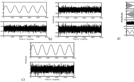
a) 0 1000 2000 3000 4000 5000 −10 −5 0 5 10 Time (n° of points) Amplitude 0 1000 2000 3000 4000 5000 −1500 −500 500 1500 b) 0 1000 2000 3000 4000 5000 −1000 −500 0 500 1000 Amplitude 0 1000 2000 3000 4000 5000 −1000 −500 0 500 1000 Time (n° of points) c) 0 1000 2000 3000 4000 5000 −2 −1 0 1 2 Time (n° of points) Amplitude 0 1000 2000 3000 4000 5000 −4 −2 0 2 4
Fig. 1. Separation of a mixture of an harmonic oscillator (0.01Hz frequency) and Gaussian noise (SNR is−20db); time (in number of points) is on x-axis, dimensionless amplitude is on y-axis: a) original sources; b) mixed signals; c) separated signals.
a) 0 2000 4000 6000 8000 10000 −5 0 5 Amplitude 0 2000 4000 6000 8000 10000 −5 0 5 0 2000 4000 6000 8000 10000 −500 0 500 0 2000 4000 6000 8000 10000 −100 0 100 Time (n° of points) 0 2000 4000 6000 8000 10000 −500 0 500 0 2000 4000 6000 8000 10000 −500 0 500 Amplitude 0 2000 4000 6000 8000 10000 −100 0 100 0 2000 4000 6000 8000 10000 −100 0 100 Time (n° of points) b) 0 2000 4000 6000 8000 10000 −2 0 2 0 2000 4000 6000 8000 10000 −2 0 2 0 2000 4000 6000 8000 10000 −2 0 2 0 2000 4000 6000 8000 10000 −5 0 5 Time (n° of points) Amplitude c)
Fig. 2. Separation of the mixture of two coupled harmonic oscilla-tors, one harmonic oscillator and Gaussian noise: a) source signals; b) mixed signals; c)separated signals;
We can observe in (Fig.1) how ICA is able to extract the harmonic oscillator from Gaussian noise with a very low signal to noise ratio (SNR = −20db). Similar results are achieved even considering different noise.
In Fig.2 we report the results related to the second exper-iment. We easily recognize as extracted signals the standard normal modes, a single harmonic oscillator and the additive noise, though the low SNR.
3.2 Nonlinear dynamical systems
We consider a particular nonlinear oscillator, i.e. the An-dronov oscillator (AnAn-dronov et al., 1966). This oscillator is a nonlinear system that generates, with suitable parameters, a limit cycle which is approached asymptotically by all other phase paths. The limit cycle is dynamically stable. It is
rep-Fig. 1. Separation of a mixture of an harmonic oscillator (0.01 Hz
frequency) and Gaussian noise (SNR is −20 db); time (in number of points) is on x-axis, dimensionless amplitude is on y-axis: (a) original sources; (b) mixed signals; (c) separated signals.
Moreover, ICA contains the following ambiguities or in-determinacies:
– we cannot determine the variances (proportional to
energies) of the independent components;
– we cannot determine the order of the independent
com-ponents.
We have used the basic model of ICA. There are, how-ever, many generalizations born along the time. Several ap-proaches have been proposed to apply ICA when the number of mixtures is less than the number of sources (Roweis, 2000; Jang and Leen, 2003). Other approaches are introduced to accomplish separation of convolved signals (signals with de-lays and echoes). Moreover, another interesting extension of the ICA could be used in the case of nonlinear mixing (Pa-junen and Karhunen, 1997; Hyv¨arinen and Pa(Pa-junen, 1999). In the next section, to show the effectiveness of basic ICA for linear mixing, we consider the ICA application to some classes of DSs.
3 Dynamical systems
DSs can be considered a general representation of large class of sequences. Then, it is very interesting and explicative as a first step to apply ICA to DSs. We consider, in particular, three types of DSs: linear, nonlinear in the regime of limit cycle, and stochastic systems, taking into account both DSs with few and infinite degrees of freedom. The linear case makes clear how ICA works. Limit cycle and stochastic sys-tems have characteristic behaviour that can be found in many geophysical systems. We have restricted our analysis to li-near/nonlinear systems which are linearly superposed. We exclude nonlinear superpositions from our analysis. They have to be treated using a different methodology (Hyv¨arinen
We have used the basic model of ICA. There are, how-ever, many generalizations born along the time. Several ap-proaches have been proposed to apply ICA when the number of mixtures is less than the number of sources (Roweis, 2000; Jang and Leen, 2003). Other approaches are introduced to accomplish separation of convolved signals (signals with de-lays and echoes). Moreover, another interesting extension of the ICA could be used in the case of nonlinear mixing (Pa-junen and Karhunen, 1997; Hyv¨arinen and Pa(Pa-junen, 1999). In the next section, to show the effectiveness of basic ICA for linear mixing, we consider the ICA application to some classes of DSs.
3 Dynamical Systems
DSs can be considered a general representation of large class of sequences. Then, it is very interesting and explicative as a first step to apply ICA to DSs. We consider, in particular, three types of DSs: linear, nonlinear in the regime of limit cycle, and stochastic systems, taking into account both DSs with few and infinite degrees of freedom. The linear case makes clear how ICA works. Limit cycle and stochastic sys-tems have characteristic behaviour that can be found in many geophysical systems. We have restricted our analysis to lin-ear/nonlinear systems which are linearly superposed. We ex-clude nonlinear superpositions from our analysis. They have to be treated using a different methodology (Hyv¨arinen and Pajunen, 1999). In fact, we have not considered nonlinear systems developing chaotic behaviour as for example Rossler attractor, in which the z-component is not well separated be-cause of the nonlinear contribution of the xz term (Ciaramella et al., 2002).
Generally, DSs are described by a first order equation sys-tem:
dx(t)
dt = F(x(t)) (5)
where F(x(t)) is a linear, nonlinear or stochastic field. In particular for stochastic systems, we consider diffusive stochastic processes described by the following equation:
dx = [v(x, t)]dt + εdW (6)
where v(x, t) is a field (drift) and dW is a Wiener process. 3.1 Linear dynamical systems
The linear systems that we analyse are single and coupled harmonic oscillators. It is enough to consider two coupled oscillators, because the behaviour of a system with many os-cillators is completely equivalent to the previous one. We have made many different experiments on mixtures gener-ated by these systems. We illustrate:
– the separation of an harmonic oscillator and an additive Gaussian noise;
– the separation of coupled oscillators, in beating regime, one harmonic oscillator and a Gaussian noise.
a) 0 1000 2000 3000 4000 5000 −10 −5 0 5 10 Time (n° of points) Amplitude 0 1000 2000 3000 4000 5000 −1500 −500 500 1500 b) 0 1000 2000 3000 4000 5000 −1000 −500 0 500 1000 Amplitude 0 1000 2000 3000 4000 5000 −1000 −500 0 500 1000 Time (n° of points) c) 0 1000 2000 3000 4000 5000 −2 −1 0 1 2 Time (n° of points) Amplitude 0 1000 2000 3000 4000 5000 −4 −2 0 2 4
Fig. 1. Separation of a mixture of an harmonic oscillator (0.01Hz frequency) and Gaussian noise (SNR is−20db); time (in number of points) is on x-axis, dimensionless amplitude is on y-axis: a) original sources; b) mixed signals; c) separated signals.
a) 0 2000 4000 6000 8000 10000 −5 0 5 Amplitude 0 2000 4000 6000 8000 10000 −5 0 5 0 2000 4000 6000 8000 10000 −500 0 500 0 2000 4000 6000 8000 10000 −100 0 100 Time (n° of points) 0 2000 4000 6000 8000 10000 −500 0 500 0 2000 4000 6000 8000 10000 −500 0 500 Amplitude 0 2000 4000 6000 8000 10000 −100 0 100 0 2000 4000 6000 8000 10000 −100 0 100 Time (n° of points) b) 0 2000 4000 6000 8000 10000 −2 0 2 0 2000 4000 6000 8000 10000 −2 0 2 0 2000 4000 6000 8000 10000 −2 0 2 0 2000 4000 6000 8000 10000 −5 0 5 Time (n° of points) Amplitude c)
Fig. 2. Separation of the mixture of two coupled harmonic oscilla-tors, one harmonic oscillator and Gaussian noise: a) source signals; b) mixed signals; c)separated signals;
We can observe in (Fig.1) how ICA is able to extract the harmonic oscillator from Gaussian noise with a very low signal to noise ratio (SNR = −20db). Similar results are achieved even considering different noise.
In Fig.2 we report the results related to the second exper-iment. We easily recognize as extracted signals the standard normal modes, a single harmonic oscillator and the additive noise, though the low SNR.
3.2 Nonlinear dynamical systems
We consider a particular nonlinear oscillator, i.e. the An-dronov oscillator (AnAn-dronov et al., 1966). This oscillator is a nonlinear system that generates, with suitable parameters, a limit cycle which is approached asymptotically by all other phase paths. The limit cycle is dynamically stable. It is
rep-Fig. 2. Separation of the mixture of two coupled harmonic
oscilla-tors, one harmonic oscillator and Gaussian noise: (a) source signals;
(b) mixed signals; (c) separated signals.
and Pajunen, 1999). In fact, we have not considered non-linear systems developing chaotic behaviour as for example R¨ossler attractor, in which the z-component is not well se-parated because of the nonlinear contribution of the xz term
(Ciaramella et al., 20021).
Generally, DSs are described by a first order equation sy-stem:
dx(t)
dt =F(x(t )), (5)
where F(x(t )) is a linear, nonlinear or stochastic field. In particular for stochastic systems, we consider diffusive stochastic processes described by the following equation:
dx = [v(x, t )]dt + εdW, (6)
where v(x, t ) is a field (drift), dW is a Wiener process and ε is the diffusion coefficient.
3.1 Linear dynamical systems
The linear systems that we analyse are single and coupled harmonic oscillators. It is enough to consider two coupled oscillators, because the behaviour of a system with many oscillators is completely equivalent to the previous one. We have made many different experiments on mixtures genera-ted by these systems. We illustrate:
– the separation of an harmonic oscillator and an additive
Gaussian noise;
– the separation of coupled oscillators, in beating regime,
one harmonic oscillator and a Gaussian noise.
1Ciaramella, A., De Lauro, E., De Martino, S., Falanga, M., and
Tagliaferri, R.: Independent Component Analysis and Dynamical Systems, Salerno University, J. Mach. Learn. Res., preprint sub-mitted, 2002.
456 A. Ciaramella et al.: Strombolian events and ICA
4 A. Ciaramella et al.: Strombolian events and ICA
resentative of many nonlinear systems with feedback. As we see in the following, this behaviour can be associated to some interesting natural systems. The equations of the Andronov oscillator with natural frequency ω0, in the suitable form, are:
¨ x + 2h1˙x + ω 2 0x = 0if x < b (7) ¨ x − 2h2˙x + ω 2 0x = 0if x > b. (8)
The nonlinearity is contained in a suitable threshold b ruling the self-coupling. We fix b = −1; h1and h2are respectively
dissipative and constructive parameters.
By using different parameters and threshold, the Andronov oscillator has different behaviours. In fact, if the threshold is negative, then we can have a limit cycle or forcing oscil-lations, while, if the threshold is positive, no limit cycle is obtained. In the other cases, for the other parameters, we have:
– 0 < h1< h2< 1: it does not have a limit cycle for any
threshold;
– b = −1 and 0 < h2 < h1 < 1: it does have a limit
cycle for any initial conditions;
– b = −1 e 0 < h2h1> 1: it does have a limit cycle for
any initial conditions.
We show a representative example to illustrate the inter-esting properties of ICA when it is applied to self-oscillating nonlinear systems. In this experiment, we consider two lin-early coupled Andronov oscillators with frequency respec-tively of 0.93Hz and 1.1Hz, one Andronov oscillator with frequency of 0.9Hz and Gaussian noise. The SNR in this case is −20 db. Applying the ICA we obtain four separated signals (Fig.3).
In conclusion linearly coupled Andronov oscillators are well separated by ICA both among them and from superim-posed noise. This experiment shows the power of ICA that is able, as in the linear case regarding the normal modes, to ex-tract the independent limit cycles in time domain. We stress that it is not trivial because the nonlinear differential equa-tions cannot be solved and FFT, due to the nonlinearity of the problem, looses its efficacy. If we lower SNR under −20 db the separation of noise is not so optimal as in linear case. 3.3 Stochastic systems
The third class of systems are stochastic diffusive processes. The archetype of models is represented by a simple symmet-ric bistable potential (double-well) driven by both an addi-tive random noise, i.e. white and Gaussian, and an exter-nal periodic bias. Given these features, the response of the system undergoes resonance-like behaviour as a function of the noise level; hence the name stochastic resonance (Gam-maitoni et al., 1998). Formally, if we consider the Langevin equation with a small periodic forcing, we obtain:
dx = [x(a − x2 ) + Acos(Ωt)]dt + εdW (9) a) 0 2000 4000 6000 8000 10000 −10 0 10 0 2000 4000 6000 8000 10000 −20 0 20 0 2000 4000 6000 8000 10000 −20 0 20 0 2000 4000 6000 8000 10000 −500 0 500 Time (n° of points) Amplitude 0 2000 4000 6000 8000 10000 −500 0 500 0 2000 4000 6000 8000 10000 −100 0 100 0 2000 4000 6000 8000 10000 −200 0 200 0 2000 4000 6000 8000 10000 −500 0 500 Time (n° of points) Amplitude b) 0 2000 4000 6000 8000 10000 −2 0 2 0 2000 4000 6000 8000 10000 −2 0 2 0 2000 4000 6000 8000 10000 −2 0 2 0 2000 4000 6000 8000 10000 −5 0 5 Time (n° of points) Amplitude c)
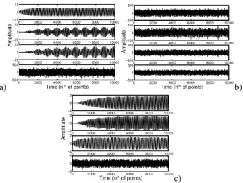
Fig. 3. Separation of the mixtures of two linearly coupled Andronov oscillators, one Andronov oscillator and Gaussian noise: a) source signals; b) mixed signals; c)separated signals.
10−3 10−2 10−1 100 −60 −40 −20 0 20 40 60 Frequency (Hz)
Power Spectrum Magnitude (dB)
10−3 10−2 10−1 100 −60 −40 −20 0 20 40 60 Frequency (Hz)
Fig. 4. Power Spectrum Density: a) a generic story of stochastic process described by eq. 9; b) z(t) described by eq. 10.
where dW is a Wiener process, i.e. a Gaussian process with zero mean and unitary variance; x is a dimensionless physi-cal variable; a is a parameter related to the double-well po-tential, A is the amplitude, Ω the angular frequency of the external periodical forcing, and ε is the diffusion coefficient. This system is compared with another that displays a sim-ilar frequency content. The latter, denoted as z(t), is de-scribed by the following equations:
¨ x = −Ω2
x
dy = νdW (10)
z(t) = Ax(t) + By(t)
where the first equation is a simple harmonic oscillator with angular frequency Ω; the second is a Wiener process; the third is the superposition of the two, according to the coeffi-cient A, B. If we choose Ω equal to the angular frequency of the stochastic process, in the regime of resonance, we obtain that z(t) has a similar frequency content as x(t) (see Fig.4).
As one can see in Fig.5, this case is very impressive, namely the separation is optimal. ICA separates low-dimensional and high-low-dimensional systems, i.e. harmonic oscillator and both stochastic resonance and Gaussian noise,
Fig. 3. Separation of the mixtures of two linearly coupled Andronov
oscillators, one Andronov oscillator and Gaussian noise: (a) source signals; (b) mixed signals; (c) separated signals.
We can observe in (Fig. 1) how ICA is able to extract the harmonic oscillator from Gaussian noise with a very low signal to noise ratio (SNR = −20 db). Similar results are achieved even considering different noise.
In Fig. 2, we report the results related to the second expe-riment. We easily recognize as extracted signals the standard normal modes, a single harmonic oscillator and the additive noise, though the low SNR.
3.2 Nonlinear dynamical systems
We consider a particular nonlinear oscillator, i.e. the An-dronov oscillator (AnAn-dronov et al., 1966). This oscillator is a nonlinear system that generates, with suitable parameters, a limit cycle which is approached asymptotically by all other phase paths. The limit cycle is dynamically stable. It is re-presentative of many nonlinear systems with feedback. As we see in the following, this behaviour can be associated to some interesting natural systems. The equations of the
An-dronov oscillator with natural frequency ω0, in the suitable
form, are:
¨
x +2h1x + ω˙ 20x =0 if x < b ¨
x −2h2x + ω˙ 20x =0 if x > b. (7)
The nonlinearity is contained in a suitable threshold b ruling
the self-coupling. We fix b = −1; h1and h2are respectively
dissipative and constructive parameters.
By using different parameters and threshold, the Andronov oscillator has different behaviours. In fact, if the threshold is negative, then we can have a limit cycle or forcing oscil-lations, while, if the threshold is positive, no limit cycle is obtained. In the other cases, for the other parameters, we have:
– 0 < h1< h2<1: it does not have a limit cycle for any
threshold;
4 A. Ciaramella et al.: Strombolian events and ICA
resentative of many nonlinear systems with feedback. As we see in the following, this behaviour can be associated to some interesting natural systems. The equations of the Andronov
oscillator with natural frequency ω0, in the suitable form, are:
¨ x + 2h1˙x + ω 2 0x = 0 if x < b (7) ¨ x − 2h2˙x + ω 2 0x = 0if x > b. (8)
The nonlinearity is contained in a suitable threshold b ruling
the self-coupling. We fix b = −1; h1and h2are respectively
dissipative and constructive parameters.
By using different parameters and threshold, the Andronov oscillator has different behaviours. In fact, if the threshold is negative, then we can have a limit cycle or forcing oscil-lations, while, if the threshold is positive, no limit cycle is obtained. In the other cases, for the other parameters, we have:
– 0 < h1< h2 < 1: it does not have a limit cycle for any
threshold;
– b = −1 and 0 < h2 < h1 < 1: it does have a limit
cycle for any initial conditions;
– b = −1 e 0 < h2h1 > 1: it does have a limit cycle for
any initial conditions.
We show a representative example to illustrate the inter-esting properties of ICA when it is applied to self-oscillating nonlinear systems. In this experiment, we consider two lin-early coupled Andronov oscillators with frequency respec-tively of 0.93Hz and 1.1Hz, one Andronov oscillator with frequency of 0.9Hz and Gaussian noise. The SNR in this case is −20 db. Applying the ICA we obtain four separated signals (Fig.3).
In conclusion linearly coupled Andronov oscillators are well separated by ICA both among them and from superim-posed noise. This experiment shows the power of ICA that is able, as in the linear case regarding the normal modes, to ex-tract the independent limit cycles in time domain. We stress that it is not trivial because the nonlinear differential equa-tions cannot be solved and FFT, due to the nonlinearity of the problem, looses its efficacy. If we lower SNR under −20 db the separation of noise is not so optimal as in linear case. 3.3 Stochastic systems
The third class of systems are stochastic diffusive processes. The archetype of models is represented by a simple symmet-ric bistable potential (double-well) driven by both an addi-tive random noise, i.e. white and Gaussian, and an exter-nal periodic bias. Given these features, the response of the system undergoes resonance-like behaviour as a function of the noise level; hence the name stochastic resonance (Gam-maitoni et al., 1998). Formally, if we consider the Langevin equation with a small periodic forcing, we obtain:
dx = [x(a − x2 ) + Acos(Ωt)]dt + εdW (9) a) 0 2000 4000 6000 8000 10000 −10 0 10 0 2000 4000 6000 8000 10000 −20 0 20 0 2000 4000 6000 8000 10000 −20 0 20 0 2000 4000 6000 8000 10000 −500 0 500 Time (n° of points) Amplitude 0 2000 4000 6000 8000 10000 −500 0 500 0 2000 4000 6000 8000 10000 −100 0 100 0 2000 4000 6000 8000 10000 −200 0 200 0 2000 4000 6000 8000 10000 −500 0 500 Time (n° of points) Amplitude b) 0 2000 4000 6000 8000 10000 −2 0 2 0 2000 4000 6000 8000 10000 −2 0 2 0 2000 4000 6000 8000 10000 −2 0 2 0 2000 4000 6000 8000 10000 −5 0 5 Time (n° of points) Amplitude c)
Fig. 3. Separation of the mixtures of two linearly coupled Andronov oscillators, one Andronov oscillator and Gaussian noise: a) source signals; b) mixed signals; c)separated signals.
10−3 10−2 10−1 100 −60 −40 −20 0 20 40 60 Frequency (Hz)
Power Spectrum Magnitude (dB)
10−3 10−2 10−1 100 −60 −40 −20 0 20 40 60 Frequency (Hz)
Fig. 4. Power Spectrum Density: a) a generic story of stochastic process described by eq. 9; b) z(t) described by eq. 10.
where dW is a Wiener process, i.e. a Gaussian process with zero mean and unitary variance; x is a dimensionless physi-cal variable; a is a parameter related to the double-well po-tential, A is the amplitude, Ω the angular frequency of the external periodical forcing, and ε is the diffusion coefficient. This system is compared with another that displays a sim-ilar frequency content. The latter, denoted as z(t), is de-scribed by the following equations:
¨
x = −Ω2
x
dy = νdW (10)
z(t) = Ax(t) + By(t)
where the first equation is a simple harmonic oscillator with angular frequency Ω; the second is a Wiener process; the third is the superposition of the two, according to the coeffi-cient A, B. If we choose Ω equal to the angular frequency of the stochastic process, in the regime of resonance, we obtain that z(t) has a similar frequency content as x(t) (see Fig.4).
As one can see in Fig.5, this case is very impressive,
namely the separation is optimal. ICA separates
low-dimensional and high-low-dimensional systems, i.e. harmonic oscillator and both stochastic resonance and Gaussian noise, Fig. 4. Power Spectrum Density: (a) a generic story of stochastic
process described by Eq. (8); (b) z(t) described by Eq. (9).
– b = −1 and 0 < h2 < h1 < 1: it does have a limit
cycle for any initial conditions;
– b = −1 e 0 < h2h1>1: it does have a limit cycle for
any initial conditions.
We show a representative example to illustrate the inte-resting properties of ICA when it is applied to self-oscillating nonlinear systems. In this experiment, we consider two li-nearly coupled Andronov oscillators with frequency respec-tively of 0.93Hz and 1.1 Hz, one Andronov oscillator with frequency of 0.9 Hz and Gaussian noise. The SNR in this case is −20 db. Applying the ICA we obtain four separated signals (Fig. 3).
In conclusion linearly coupled Andronov oscillators are well separated by ICA both among them and from superim-posed noise. This experiment shows the power of ICA that is able, as in the linear case regarding the normal modes, to ex-tract the independent limit cycles in time domain. We stress that it is not trivial because the nonlinear differential equa-tions cannot be solved and FFT, due to the nonlinearity of the problem, looses its efficacy. If we lower SNR under −20 db the separation of noise is not so optimal as in linear case.
3.3 Stochastic systems
The third class of systems are stochastic diffusive processes. The archetype of models is represented by a simple symme-tric bistable potential (double-well) driven by both an ad-ditive random noise, i.e. white and Gaussian, and an exter-nal periodic bias. Given these features, the response of the system undergoes resonance-like behaviour as a function of the noise level; hence the name stochastic resonance (Gam-maitoni et al., 1998). Formally, if we consider the Langevin equation with a small periodic forcing, we obtain:
dx = [x(a − x2) + Acos(t )]dt + εdW, (8) where dW is a Wiener process, i.e. a Gaussian process with zero mean and unitary variance; x is a dimensionless physi-cal variable; a is a parameter related to the double-well po-tential, A is the amplitude, the angular frequency of the external periodical forcing, and ε is the diffusion coefficient. This system is compared with another that displays a si-milar frequency content. The latter, denoted as z(t), is de-scribed by the following equations:
0 1 2 3 4 5 x 10⁴ −10 0 10 0 1 2 3 4 5 x 10⁴ −2 0 2 0 1 2 3 4 5 x 10⁴ −5 0 5 Time (n° of points) Amplitude a) 0 1 2 3 4 5 x 10⁴ −10 0 10 0 1 2 3 4 5 x 10⁴ −10 0 10 0 1 2 3 4 5 x 10⁴ −10 0 10 Time (n° of points) Amplitude b) 0 1 2 3 4 5 x 10⁴ −2 0 2 0 500 1000 1500 2000 −2 0 2 0 1 2 3 4 5 x 10⁴ −5 0 5 Time (n° of points) Amplitude c)
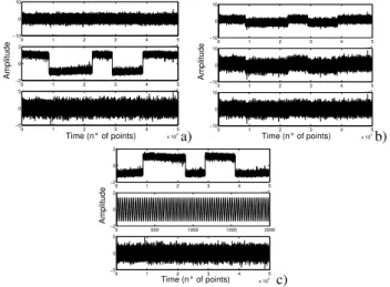
Fig. 5. Separation of the mixture of linear oscillator with frequency of 0.003Hz with an additive Gaussian noise and stochastic reso-nance with the same resoreso-nance frequency: a) source signals; b) mixed signals; c) extracted components.
also in presence of a very similar frequency content. Same results are achieved using different kinds of noise (e.g. uni-form noise). Obviously, ICA is not able to recognize the number of degrees of freedom and if we consider real sys-tems for which we have not ”a priori” knowledge, we must add to ICA other independent methods (De Martino et al., 2002c).
We should note that linear methods based on FFT fail, because they do not distinguish the systems underlying our mixtures, describing the observed spectra as due to the same DS. In that framework, a stochastic resonance is not at all different from a simple oscillator with noise. The ICA well distinguishes the case in which the harmonic oscillator is lin-early superposed to noise from the case in which the FFT peak is generated by a stochastic behaviour, i.e. stochastic resonance.
Now we can draw our conclusions about the explicative synthetic examples. We have applied ICA to some dynami-cal systems; firstly to linear and nonlinear systems with few degrees of freedom, and then to infinite degrees of freedom systems, namely diffusion processes in the regime of stochas-tic resonance.
Regarding the linear systems, we have obtained optimal sep-aration from very high superposed noise. Furthermore, the ICA acts as Fast Fourier Transform but in time domain since it gives us the normal modes of the system.
The performance of ICA is valuable also in the case of non-linear systems where we separate coupled Andronov oscil-lators, not trivial from the point of view of dynamical sys-tems. Also in these experiments the separation from noise is well made. The experiments with stochastic resonance are very impressive: the superposed periodic and stochastic sig-nals are completely separated, i.e. ICA perfectly recognizes the different superposed dynamical systems also when the Fourier Transform is irresolute (insensitive). As a conclusive
0 100 200 300 400 500 600 700 800 900 −4 −3 −2 −1 0x 104 0 100 200 300 400 500 600 700 800 900 −5000 0 5000 Time (s) Amplitude (counts)
Fig. 6. In the upper figure, 15 minutes of the vertical component of broadband event is plotted (amplitudes in adimensional unit). It was recorded at T1 station on September 19th
at 22:00, during the ex-periment performed in 1997, where 21 three-component broadband seismometers were deployed on the flanks of the volcano, grouped into three rings at different levels: Top, Middle, Bottom stations. In the lower figure, the same event is filtered in the band 0.02−0.5Hz, in order to make evident the waveform of the explosions superposed to background tremor.
remark we can say that ICA is a method to apply a priori as a pre-analysis to scalar experimental series, namely it allows to recognize if the scalar series contain one or more indepen-dent signals.
4 Application of ICA to Strombolian events
We study the seismic signals recorded at Stromboli volcano. This volcano is characterized by basaltic eruptions. In these eruptions, the relative motion of gas with respect to the fluid produces either an annular flow (Hawaian Fire Fountains) or a Slug flow (Strombolian explosions). In fact, the typi-cal seismic signature of Stromboli is the continuous volcanic tremor (continuous vibration of the ground around the vol-cano) due to degassing to which repeating explosion quakes are superposed (see Fig.6).
Tremor and explosions have a very similar frequency con-tent. In fact, both the behaviours are generated by complex processes of magma flow and turbulent degassing.
Despite many studies (e.g. Chouet et al., 1997, 1999, 2003), the dynamics underlying the generation of these be-haviours is not yet well understood.
In our studies, we have applied ICA to Strombolian events considering both short-period (0.5 − 50Hz) and broadband (0.02 − 50Hz) recorded seismograms. Strombolian signals, due to their stationarity, are suitable to apply ICA. The aim is to decompose, if it is possible, recorded series into statis-tically independent components. In this way, we get infor-mation about the ”modes” involved in the full dynamics and constrain source geometry and mechanism. The analysis will be carried on explosions and tremor, separately.
In order to avoid any delay among recording stations located in different places, the seismic traces are aligned using the
Fig. 5. Separation of the mixture of linear oscillator with frequency
of 0.003 Hz with an additive Gaussian noise and stochastic reso-nance with the same resoreso-nance frequency: (a) source signals; (b) mixed signals; (c) extracted components.
¨
x = −2x
dy = εdW (9)
z(t ) = Ax(t ) + By(t ),
where the first equation is a simple harmonic oscillator with angular frequency ; the second is a Wiener process; the third is the superposition of the two, according to the coeffi-cient A, B. If we choose equal to the angular frequency of the stochastic process, in the regime of resonance, we obtain that z(t ) has a similar frequency content as x(t) (see Fig. 4). As one can see in Fig. 5, this case is very impres-sive, namely the separation is optimal. ICA separates low-dimensional and high-low-dimensional systems, i.e. harmonic os-cillator and both stochastic resonance and Gaussian noise, also in presence of a very similar frequency content. Same results are achieved using different kinds of noise (e.g. uni-form noise). Obviously, ICA is not able to recognize the number of degrees of freedom and if we consider real sy-stems for which we have not “a priori” knowledge, we must add to ICA other independent methods (De Martino et al., 2002c).
We should note that linear methods based on FFT fail, because they do not distinguish the systems underlying our mixtures, describing the observed spectra as due to the same DS. In that framework, a stochastic resonance is not at all different from a simple oscillator with noise. The ICA well distinguishes the case in which the harmonic oscillator is li-nearly superposed to noise from the case in which the FFT peak is generated by a stochastic behaviour, i.e. stochastic resonance.
Now we can draw our conclusions about the explicative synthetic examples. We have applied ICA to some dynami-cal systems; firstly to linear and nonlinear systems with few degrees of freedom, and then to infinite degrees of freedom
0 1 2 3 4 5 x 10⁴ −10 0 10 0 1 2 3 4 5 x 10⁴ −2 0 2 0 1 2 3 4 5 x 10⁴ −5 0 5 Time (n° of points) Amplitude a) 0 1 2 3 4 5 x 10⁴ −10 0 10 0 1 2 3 4 5 x 10⁴ −10 0 10 0 1 2 3 4 5 x 10⁴ −10 0 10 Time (n° of points) Amplitude b) 0 1 2 3 4 5 x 10⁴ −2 0 2 0 500 1000 1500 2000 −2 0 2 0 1 2 3 4 5 x 10⁴ −5 0 5 Time (n° of points) Amplitude c)
Fig. 5. Separation of the mixture of linear oscillator with frequency of 0.003Hz with an additive Gaussian noise and stochastic reso-nance with the same resoreso-nance frequency: a) source signals; b) mixed signals; c) extracted components.
also in presence of a very similar frequency content. Same results are achieved using different kinds of noise (e.g. uni-form noise). Obviously, ICA is not able to recognize the number of degrees of freedom and if we consider real sys-tems for which we have not ”a priori” knowledge, we must add to ICA other independent methods (De Martino et al., 2002c).
We should note that linear methods based on FFT fail, because they do not distinguish the systems underlying our mixtures, describing the observed spectra as due to the same DS. In that framework, a stochastic resonance is not at all different from a simple oscillator with noise. The ICA well distinguishes the case in which the harmonic oscillator is lin-early superposed to noise from the case in which the FFT peak is generated by a stochastic behaviour, i.e. stochastic resonance.
Now we can draw our conclusions about the explicative synthetic examples. We have applied ICA to some dynami-cal systems; firstly to linear and nonlinear systems with few degrees of freedom, and then to infinite degrees of freedom systems, namely diffusion processes in the regime of stochas-tic resonance.
Regarding the linear systems, we have obtained optimal sep-aration from very high superposed noise. Furthermore, the ICA acts as Fast Fourier Transform but in time domain since it gives us the normal modes of the system.
The performance of ICA is valuable also in the case of non-linear systems where we separate coupled Andronov oscil-lators, not trivial from the point of view of dynamical sys-tems. Also in these experiments the separation from noise is well made. The experiments with stochastic resonance are very impressive: the superposed periodic and stochastic sig-nals are completely separated, i.e. ICA perfectly recognizes the different superposed dynamical systems also when the Fourier Transform is irresolute (insensitive). As a conclusive
0 100 200 300 400 500 600 700 800 900 −4 −3 −2 −1 0x 10 4 0 100 200 300 400 500 600 700 800 900 −5000 0 5000 Time (s)
Amplitude (counts)
Fig. 6. In the upper figure, 15 minutes of the vertical component of broadband event is plotted (amplitudes in adimensional unit). It was recorded at T1 station on September 19th
at 22:00, during the ex-periment performed in 1997, where 21 three-component broadband seismometers were deployed on the flanks of the volcano, grouped into three rings at different levels: Top, Middle, Bottom stations. In the lower figure, the same event is filtered in the band 0.02−0.5Hz, in order to make evident the waveform of the explosions superposed to background tremor.
remark we can say that ICA is a method to apply a priori as a pre-analysis to scalar experimental series, namely it allows to recognize if the scalar series contain one or more indepen-dent signals.
4 Application of ICA to Strombolian events
We study the seismic signals recorded at Stromboli volcano. This volcano is characterized by basaltic eruptions. In these eruptions, the relative motion of gas with respect to the fluid produces either an annular flow (Hawaian Fire Fountains) or a Slug flow (Strombolian explosions). In fact, the typi-cal seismic signature of Stromboli is the continuous volcanic tremor (continuous vibration of the ground around the vol-cano) due to degassing to which repeating explosion quakes are superposed (see Fig.6).
Tremor and explosions have a very similar frequency con-tent. In fact, both the behaviours are generated by complex processes of magma flow and turbulent degassing.
Despite many studies (e.g. Chouet et al., 1997, 1999, 2003), the dynamics underlying the generation of these be-haviours is not yet well understood.
In our studies, we have applied ICA to Strombolian events considering both short-period (0.5 − 50Hz) and broadband (0.02 − 50Hz) recorded seismograms. Strombolian signals, due to their stationarity, are suitable to apply ICA. The aim is to decompose, if it is possible, recorded series into statis-tically independent components. In this way, we get infor-mation about the ”modes” involved in the full dynamics and constrain source geometry and mechanism. The analysis will be carried on explosions and tremor, separately.
In order to avoid any delay among recording stations located in different places, the seismic traces are aligned using the Fig. 6. In the upper figure, 15 minutes of the vertical component
of broadband event is plotted (amplitudes in adimensional unit). It was recorded at T1 station on 19 September at 22:00, during the ex-periment performed in 1997, where 21 three-component broadband seismometers were deployed on the flanks of the volcano, grouped into three rings at different levels: Top, Middle, Bottom stations. In the lower figure, the same event is filtered in the band 0.02−0.5 Hz, in order to make evident the waveform of the explosions superposed to background tremor.
systems, namely diffusion processes in the regime of stochas-tic resonance.
Regarding the linear systems, we have obtained optimal separation from very high superposed noise. Furthermore, the ICA acts as Fast Fourier Transform but in time domain since it gives us the normal modes of the system.
The performance of ICA is valuable also in the case of nonlinear systems where we separate coupled Andronov os-cillators, not trivial from the point of view of dynamical sy-stems. Also in these experiments, the separation from noise is well made. The experiments with stochastic resonance are very impressive: the superposed periodic and stochastic sig-nals are completely separated, i.e. ICA perfectly recognizes the different superposed dynamical systems also when the Fourier Transform is irresolute (insensitive). As a conclusive remark, we can say that ICA is a method to apply “a pri-ori” as a pre-analysis to scalar experimental series, namely it allows to recognize if the scalar series contain one or more independent signals.
4 Application of ICA to Strombolian events
We study the seismic signals recorded at Stromboli volcano. This volcano is characterized by basaltic eruptions. In these eruptions, the relative motion of gas with respect to the fluid produces either an annular flow (Hawaian Fire Fountains) or a Slug flow (Strombolian explosions). In fact, the typi-cal seismic signature of Stromboli is the continuous volcanic tremor (continuous vibration of the ground around the vol-cano) due to degassing to which repeating explosion quakes are superposed (see Fig. 6).
458 A. Ciaramella et al.: Strombolian events and ICA
6 A. Ciaramella et al.: Strombolian events and ICA
cross-correlation function. This satisfies the ICA request of instantaneous mixing.
To get other information, we have also adopted differ-ent techniques. They consist in techniques generally used in nonlinear signal processing, and well-known or innova-tive methods to investigate seismological signals. In partic-ular, we have applied parametric and non parametric spec-tral analysis; nonlinear denoising techniques (Kostelich and Schreiber, 1993); particle motion and polarization filtering (Kanasewich, 1981); methods to reconstruct phase space starting from scalar time series (estimate of the dimension (Grassberger and Procaccia, 1983), Average Mutual Infor-mation (Fraser and Swinney, 1986), False Nearest Neighbors (Kennel et al., 1992)); trajectory space analysis to estimate the variety of dynamical systems presents in the data (Pal-adin and Vulpiani, 1987).
As regards explosions at high frequency, we report the re-sults obtained decomposing signals recorded by using short-period seismometers (Chouet et al., 1998). ICA has been ap-plied to explosions recorded by seismometers along the three orthonormal directions of motion, i.e. radial, transverse, ver-tical with respect to the crater area.
We display in Fig.7 the results of the radial direction; the other directions show a similar behaviour (Acernese et al., 2003). As one can see (Fig.7), the wavefield is the linear superposition in time domain of three independent compo-nents, characterized by well defined and separate frequency bands (respectively 0.8 − 1.2, 2.4 − 3.0, 3.2 − 4.5Hz).
The first two bands present wavefield mainly composed of body waves with radial polarization, pointing towards the crater area. In the last band, the very low SNR, together with the corresponding short wavelengths, does not allow to indi-viduate a defined direction (Acernese et al., 2004).
Similar results are achieved analysing broadband explo-sions. In addition, in this case, we extract also a component corresponding to the VLP signal (Falanga, 2003) as already observed by Chouet et al. (2003).
The reconstruction of the phase space establishes that ex-plosions are associated to a low-dimensional dynamical sys-tem characterized by dimensions in the range [2 − 3] (De Martino et al., 2002a).
Then, trajectory space analysis, performed on broadband signals, states that explosions are generated by an unique dy-namical system (De Martino et al., 2004), though Chouet et al. (2003) have found two distinct kinds of explosions, which have been associated to the two distinct vents at Stromboli in 1997. The differences between the two types of events are related more to slight variations in conduit ge-ometries rather than differences in the dynamics generation of the phenomena.
We have also analysed, as already said, the tremor. In this case, it is convenient to consider separately two frequency bands (> 0.5Hz and < 0.5Hz). Namely, the low frequency band can contain waves travelling with different velocity with respect to the high frequency wavefield. In Fig.8, as you can see, tremor shows ICA extracted components similar to explosion quakes, in waveform and frequency content. Of
0 2 4 6 0 2 4 6
PSD
0 2 4 6 0 1 2 Frequency (Hz) 0 2 4 6 0 20 40 60 0 1000 2000 3000 −1 0 1Amplitude
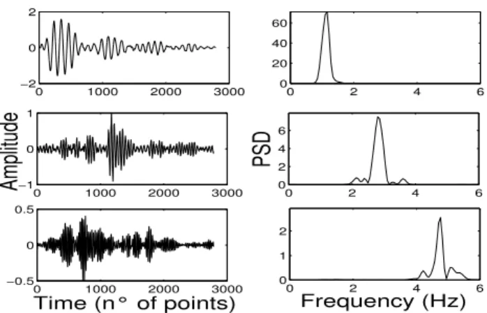
0 1000 2000 3000 −0.5 0 0.5 Time (n° of points) 0 1000 2000 3000 −2 0 2Fig. 7. Explosions in the band greater than 0.5Hz: Denoised inde-pendent components of radial direction of motion and their spectra (sampling frequency equal to 125Hz; amplitude in adimensional unit. 0 1 2 3 4 5 6 7 8 0 20 40 60 80 20 40 60 80 −1 0 1 0 1 2 3 4 5 6 7 8 0 20 40
PDS
20 40 60 80 −1 0 1Amplitude(a.u.)
0 1 2 3 4 5 6 7 8 0 20 40 Frequency(Hz) 20 40 60 80 −1 0 1 Time(s)Fig. 8. Denoised independent components of tremor, by ICA, in the range > 0.5Hz related to the vertical direction and their spectra; amplitude in adimensional unit.
course, regarding tremor, the individuation of clear bands is more difficult due to very low SNR. Polarization analysis on tremor has already been performed on short-period recorded signals Chouet et al. (1997). We are extending the analysis to broadband signals as extracted by ICA. This will be matter of a forthcoming paper.
All the results persuade us to think that, regarding high frequency content, the superficial source is stationary and not destructive. The wavefield is generated by the excita-tion of only feww degrees of freedom of the complex fluid-dynamical source system.
Possible models of the production of these oscillations have been postulated by Julian (1994), Ida (1996) and James et al. (2004). In particular, Julian (1994) suggested an or-gan pipe model, with a constant rate supply of fluids inside a cylinder conduit for a variety of almost periodic signals ob-served on volcanoes.
The independent component analysis of organ pipe acous-tic emission by Bottiglieri et al. (2004) seems to support this model. Namely, in an organ pipe, a constant rate supply of pressure produces self-sustained sounds and ICA is able Fig. 7. Explosions in the band greater than 0.5 Hz: Denoised
inde-pendent components of radial direction of motion and their spectra (sampling frequency equal to 125 Hz; amplitude in adimensional unit).
Tremor and explosions have a very similar frequency con-tent. In fact, both the behaviours are generated by complex processes of magma flow and turbulent degassing.
Despite many studies (e.g. Chouet et al., 1997, 1999, 2003), the dynamics underlying the generation of these be-haviours is not yet well understood.
In our studies, we have applied ICA to Strombolian events considering both short-period (0.5−50 Hz) and broadband (0.02−50 Hz) recorded seismograms. Strombolian signals, due to their stationarity, are suitable to apply ICA. The aim is to decompose, if it is possible, recorded series into stati-stically independent components. In this way, we get infor-mation about the “modes” involved in the full dynamics and constrain source geometry and mechanism. The analysis will be carried on explosions and tremor, separately.
In order to avoid any delay among recording stations lo-cated in different places, the seismic traces are aligned using the cross-correlation function. This satisfies the ICA request of instantaneous mixing.
To get other information, we have also adopted different techniques. They consist in techniques generally used in nonlinear signal processing, and well-known or innovative
methods to investigate seismological signals. In
particu-lar, we have applied parametric and non parametric spec-tral analysis; nonlinear denoising techniques (Kostelich and Schreiber, 1993); particle motion and polarization filtering (Kanasewich, 1981); methods to reconstruct phase space starting from scalar time series (estimate of the dimension (Grassberger and Procaccia, 1983), Average Mutual Infor-mation (Fraser and Swinney, 1986), False Nearest Neighbors (Kennel et al., 1992)); trajectory space analysis to estimate the variety of dynamical systems presents in the data (Pal-adin and Vulpiani, 1987).
As regards explosions at high frequency, we report the re-sults obtained decomposing signals recorded by using short-period seismometers (Chouet et al., 1998). ICA has been ap-plied to explosions recorded by seismometers along the three
6 A. Ciaramella et al.: Strombolian events and ICA
cross-correlation function. This satisfies the ICA request of instantaneous mixing.
To get other information, we have also adopted differ-ent techniques. They consist in techniques generally used in nonlinear signal processing, and well-known or innova-tive methods to investigate seismological signals. In partic-ular, we have applied parametric and non parametric spec-tral analysis; nonlinear denoising techniques (Kostelich and Schreiber, 1993); particle motion and polarization filtering (Kanasewich, 1981); methods to reconstruct phase space starting from scalar time series (estimate of the dimension (Grassberger and Procaccia, 1983), Average Mutual Infor-mation (Fraser and Swinney, 1986), False Nearest Neighbors (Kennel et al., 1992)); trajectory space analysis to estimate the variety of dynamical systems presents in the data (Pal-adin and Vulpiani, 1987).
As regards explosions at high frequency, we report the re-sults obtained decomposing signals recorded by using short-period seismometers (Chouet et al., 1998). ICA has been ap-plied to explosions recorded by seismometers along the three orthonormal directions of motion, i.e. radial, transverse, ver-tical with respect to the crater area.
We display in Fig.7 the results of the radial direction; the other directions show a similar behaviour (Acernese et al., 2003). As one can see (Fig.7), the wavefield is the linear superposition in time domain of three independent compo-nents, characterized by well defined and separate frequency bands (respectively 0.8 − 1.2, 2.4 − 3.0, 3.2 − 4.5Hz).
The first two bands present wavefield mainly composed of body waves with radial polarization, pointing towards the crater area. In the last band, the very low SNR, together with the corresponding short wavelengths, does not allow to indi-viduate a defined direction (Acernese et al., 2004).
Similar results are achieved analysing broadband explo-sions. In addition, in this case, we extract also a component corresponding to the VLP signal (Falanga, 2003) as already observed by Chouet et al. (2003).
The reconstruction of the phase space establishes that ex-plosions are associated to a low-dimensional dynamical sys-tem characterized by dimensions in the range [2 − 3] (De Martino et al., 2002a).
Then, trajectory space analysis, performed on broadband signals, states that explosions are generated by an unique dy-namical system (De Martino et al., 2004), though Chouet et al. (2003) have found two distinct kinds of explosions, which have been associated to the two distinct vents at Stromboli in 1997. The differences between the two types of events are related more to slight variations in conduit ge-ometries rather than differences in the dynamics generation of the phenomena.
We have also analysed, as already said, the tremor. In this case, it is convenient to consider separately two frequency bands (> 0.5Hz and < 0.5Hz). Namely, the low frequency band can contain waves travelling with different velocity with respect to the high frequency wavefield. In Fig.8, as you can see, tremor shows ICA extracted components similar to explosion quakes, in waveform and frequency content. Of
0 2 4 6 0 2 4 6
PSD
0 2 4 6 0 1 2 Frequency (Hz) 0 2 4 6 0 20 40 60 0 1000 2000 3000 −1 0 1Amplitude
0 1000 2000 3000 −0.5 0 0.5 Time (n° of points) 0 1000 2000 3000 −2 0 2Fig. 7. Explosions in the band greater than 0.5Hz: Denoised inde-pendent components of radial direction of motion and their spectra (sampling frequency equal to 125Hz; amplitude in adimensional unit. 0 1 2 3 4 5 6 7 8 0 20 40 60 80 20 40 60 80 −1 0 1 0 1 2 3 4 5 6 7 8 0 20 40
PDS
20 40 60 80 −1 0 1Amplitude(a.u.)
0 1 2 3 4 5 6 7 8 0 20 40 Frequency(Hz) 20 40 60 80 −1 0 1 Time(s)Fig. 8. Denoised independent components of tremor, by ICA, in the range > 0.5Hz related to the vertical direction and their spectra; amplitude in adimensional unit.
course, regarding tremor, the individuation of clear bands is more difficult due to very low SNR. Polarization analysis on tremor has already been performed on short-period recorded signals Chouet et al. (1997). We are extending the analysis to broadband signals as extracted by ICA. This will be matter of a forthcoming paper.
All the results persuade us to think that, regarding high frequency content, the superficial source is stationary and not destructive. The wavefield is generated by the excita-tion of only feww degrees of freedom of the complex fluid-dynamical source system.
Possible models of the production of these oscillations have been postulated by Julian (1994), Ida (1996) and James et al. (2004). In particular, Julian (1994) suggested an or-gan pipe model, with a constant rate supply of fluids inside a cylinder conduit for a variety of almost periodic signals ob-served on volcanoes.
The independent component analysis of organ pipe acous-tic emission by Bottiglieri et al. (2004) seems to support this model. Namely, in an organ pipe, a constant rate supply of pressure produces self-sustained sounds and ICA is able Fig. 8. Denoised independent components of tremor, by ICA, in
the range >0.5 Hz related to the vertical direction and their spectra (amplitude in adimensional unit).
orthonormal directions of motion, i.e. radial, transverse, ver-tical with respect to the crater area.
We display in Fig. 7 the results of the radial direction; the other directions show a similar behaviour (Acernese et al., 2003). As one can see (Fig. 7), the wavefield is the linear superposition in time domain of three independent compo-nents, characterized by well defined and separate frequency bands (respectively 0.8−1.2, 2.4−3.0, 3.2−4.5 Hz).
The first two bands present wavefield mainly composed of body waves with radial polarization, pointing towards the crater area. In the last band, the very low SNR, together with the corresponding short wavelengths, does not allow to indi-viduate a defined direction (Acernese et al., 2004).
Similar results are achieved analysing broadband explo-sions. In addition, in this case, we extract also a component corresponding to the VLP signal (Falanga, 2003) as already observed by Chouet et al. (2003).
The reconstruction of the phase space establishes that ex-plosions are associated to a low-dimensional dynamical sy-stem characterized by dimensions in the range [2−3] (De Martino et al., 2002a).
Then, trajectory space analysis, performed on broadband signals, states that explosions are generated by an unique dy-namical system (De Martino et al., 2004), though Chouet et al. (2003) have found two distinct kinds of explosions, which have been associated to the two distinct vents at Stromboli in 1997. The differences between the two types of events are related more to slight variations in conduit geo-metries rather than differences in the dynamics generation of the phenomena.
We have also analysed, as already said, the tremor. In this case, it is convenient to consider separately two frequency bands (> 0.5 Hz and < 0.5 Hz). Namely, the low frequency band can contain waves travelling with different velocity with respect to the high frequency wavefield. In Fig. 8, as you can see, tremor shows ICA extracted components similar to explosion quakes, in waveform and frequency content. Of course, regarding tremor, the individuation of clear bands is
![Fig. 9. Denoised independent components by ICA in the range [ 0.02 − 0.5Hz ] of vertical direction of motion and their spectra;](https://thumb-eu.123doks.com/thumbv2/123doknet/14801174.606340/8.892.466.814.92.312/denoised-independent-components-range-vertical-direction-motion-spectra.webp)
