CONTROLS ON EARTHQUAKE RUPTURE AND TRIGGERING MECHANISMS IN SUBDUCTION ZONES
By
Andrea Lesley Llenos
Sc.B., Brown University, 2004
Submitted in partial fulfillment of the requirements for the degree of Doctor of Philosophy
at the
MASSACHUSETTS INSTITUTE OF TECHNOLOGY
and the
WOODS HOLE OCEANOGRAPHIC INSTITUTION
June 2010
0 2010 Andrea L. Llenos All rights reserved.
ARCHNES
MASSACHUSETTS INST[TUTE
OF TECHNOLOGY
JUN 2
8
2010
LIBRARIES
The author hereby grants to MIT and WHOI permission to reproduce andto distribute publicly paper and electronic copies of this thesis document in whole or in part in any medium now known or hereafter created.
Author... &... ...
Joint Program in Oceanography/Applied Ocean Science and Engineering Massachusetts Institute o Technology and Woods Hole Oceanographic Institution
A // n IIebruary 12, 2010
Certified by... ...
...---.-Jeffrey J. McGuire Associate Scientist, Department of Geology and Geophysics, WHOI
19 Thesis supervisor
Accepted by...
Bradford H. Hager Professor, Department of Earth, Atmospheric, and Planetary Science, MIT Co-chair, Joint Committee for Geology and Geophysics
CONTROLS ON EARTHQUAKE RUPTURE AND TRIGGERING MECHANISMS IN SUBDUCTION ZONES
By
Andrea Lesley Llenos
Submitted to the MIT/WHOI Joint Program in Oceanography/Applied Ocean Science and Engineering on February 12, 2010 in partial fulfillment of the requirements for the
degree of Doctor of Philosophy in Marine Geophysics
Abstract
Large earthquake rupture and triggering mechanisms that drive seismicity in subduction zones are investigated in this thesis using a combination of earthquake observations, statistical and physical modeling. A comparison of the rupture
characteristics of M 7.5 earthquakes with fore-arc geological structure suggests that
long-lived frictional heterogeneities (asperities) are primary controls on the rupture extent of large earthquakes. To determine when and where stress is accumulating on the megathrust that could cause one of these asperities to rupture, this thesis develops a new method to invert earthquake catalogs to detect space-time variations in stressing rate. This algorithm is based on observations that strain transients due to aseismic processes such as fluid flow, slow slip, and afterslip trigger seismicity, often in the form of earthquake swarms. These swarms are modeled with two common approaches for investigating time-dependent driving mechanisms in earthquake catalogs: the stochastic Epidemic Type Aftershock Sequence model [Ogata, 1988] and the physically-based rate-state friction model [Dieterich, 1994]. These approaches are combined into a single model that accounts for both aftershock activity and variations in background seismicity rate due to aseismic processes, which is then implemented in a data assimilation algorithm to invert catalogs for space-time variations in stressing rate. The technique is evaluated with a synthetic test and applied to catalogs from the Salton Trough in southern California and the Hokkaido corner in northeastern Japan. The results demonstrate that the algorithm can successfully identify aseismic transients in a multi-decade earthquake catalog, and may also ultimately be useful for mapping spatial variations in frictional conditions on the plate interface.
Thesis supervisor: Dr. Jeffrey J. McGuire Title: Associate Scientist with Tenure
This thesis would not have been possible without the help and support of many, many people over the past six years, only a few of whom can be listed here. First and foremost, my deepest thanks go to my advisor Jeff McGuire, for all his time, support, confidence, patience, tolerance and nudging when I needed it. I have learned a tremendous amount from him and look forward to continuing to do so throughout the rest of my scientific career. I am also grateful for the help and insights provided by my thesis committee: Jian Lin, Rob Reves-Sohn, and Brad Hager, and thank Greg Hirth for chairing my defense. I would also like to thank current and former members of G&G and the EAPS Geophysics group, especially Laurent Montesi, Mark Behn, Dan Lizarralde, Stephane Rondenay and Brian Evans. I learned a lot from my various interactions with them in seminars, classes, projects, casual chats, and field trips. I'm also grateful for my fellow JP G&G and EAPS students, and in particular my group-mate, Emily Roland.
I have benefited a great deal from working with Yosihiko Ogata and Jiancang
Zhuang at the Institute of Statistical Mathematics in Tokyo, Japan, who taught me a lot about the ETAS model and were gracious hosts during my two visits to the ISM. Thanks also go to Koichi Katsura, Akiko Kutsuna and the rest of the Statistical Seismology group at ISM.
I greatly appreciate the efforts of the WHOI Academic Programs Office,
especially Julia and Marsha; the MIT Education Office, especially Ronni, Carol, and Jacqui; the WHOI G&G Administrative staff, especially Christina and Maryanne; the
EAPS Administrative staff, especially Beth and Kerin; and WHOI CIS, especially Jeff D.
and Jonathan. Their assistance over the years has been invaluable. I'd also like to thank Andrew Daly for his organizational work on all the Geodynamics field trips I was able to participate in and our numerous talks about international travel, and Rose for the friendly and encouraging chats.
Staying sane in grad school would have been much harder without the support and friendships I have found in the various groups I've been involved in over the years, in particular FloodSafe Honduras, the Tech Catholic Community, the MIT Warehouse Music Program, and the MIT Women's Chorale. I'm extraordinarily grateful for my friends up in Boston, throughout New England and beyond, particularly Sunita, Linda, Gail, Joanne, and Wan, who were very good at making sure I left my computer from time to time. A special thank you goes to Elizabeth, friend, roommate, and all-around partner-in-crime over the last few years, for so many things that I will sum up simply as "being there." Grad school would have been significantly less fun and more difficult without her help and support. Finally, much thanks and love to my family, especially my sister Tracy and my mom, for supporting me even while wondering what exactly I was up to. Their constant love and support has made it possible for me to get this far.
Funding for this research was provided by a WHOI Hollister Research Fellowship, a National Defense Science and Engineering Graduate Fellowship, National Science Foundation Division of Earth Sciences (EAR) grant #0738641, United States
Geological Survey National Earthquake Hazards Reduction Program Award
Table of Contents
A bstract... . 3
Acknowledgments...4
Chapter 1: Introduction...9
Chapter 2: Influence of fore-arc structure on the rupture extent of great subduction zone earthquakes... 17
1 Introduction... 18
2 M ethodology... 20
3 R esults... 25
3.1 The 2003 Colima Mexico earthquake...25
3.2 The 2006 Java earthquake...26
3.3 The 1995 Chile earthquake...27
3.4 Evaluation of bias from unmodeled propagation effects...28
3.5 Summary of results...29
4 D iscussion... 29
4.1 Fore-arc basin formation and wedge mechanics...30
4.2 How great earthquakes stop: Dynamic versus quenched heterogeneity...31
5 C onclusion... 33
Appendix A: One-dimensional versus three-dimensional synthetics...34
Appendix B: Results from additional events... 47
Chapter 3: Modeling seismic swarms triggered by aseismic transients...49
1 Introduction...50
2 M odels... 5 1 2.1 ETAS model ... 52
2.3 Combining the ETAS and rate-state models...54
3 D ata analysis... 55
3.1 Detection of anomalous seismicity rates...55
3.1.1 2005 Obsidian Buttes swarm...55
3.1.2 2005 Kilauea swarm...56
3.1.3 2002 and 2007 Boso swarms...56
3.2 Fitting ETAS to earthquake swarms...57
3.3 Comparison of rate-state predictions with observations...58
3.4 Sum m ary...58
4 Discussion and conclusion...58
Chapter 4: Detecting aseismic strain transients from seismicity data...61
1 Introduction...62
2 M ethod ... 64
2.1 ETAS model...65
2.2 Rate- and state-dependent friction model...66
2.3 Combined ETAS/rate-state model...66
2.4 Extended Kalman Filter algorithm... 67
2.5 Likelihood calculations...69
2.6 Sum m ary...70
3 Synthetic test... 71
3.1 Parameter estimation...71
3.2 Synthetic test results...73
4 Data analysis: Salton Trough...74
4.1 D ata binning... 74
4.2 Parameter estimation...75
4.3 R esults... 76
6 C onclusion... 78
Chapter 5: Detecting aseismic transients in the Hokkaido corner... 95
1 Introduction...96
2 M ethod ... 97
3 Data analysis and results...99
3.1 ETAS fitting to aftershock sequences...99
3.2 Filter results...10 1 3.2.1 Afterslip of the 1989 M7.1 and 1992 M6.9 Sanriku-oki earthquakes...102
3.2.2 Afterslip of the 1994 M7.6 Sanriku-oki earthquake...102
3.2.3 Afterslip of the 2003 M8.0 Tokachi-oki earthquake...103
3.2.4 Afterslip following moderate earthquakes...104
4 D iscussion ... 104
Chapter 1: Introduction
The largest earthquakes in the world occur on the megathrust of subduction zones, where almost 90% of the total seismic moment is released [Pacheco and Sykes, 1992]. Therefore, understanding the controls on large earthquake rupture and the triggering mechanisms that affect earthquake occurrence, in general, is critical in order to accurately assess both long-term and short-term seismic hazards in these regions. A wide spectrum of deformation occurs in subduction zones, ranging from the seismic (e.g., low frequency events, seismic tremor, microearthquakes, moderate-to-great interplate earthquakes) to the aseismic (e.g., stable slip, slow slip events, afterslip). All of these processes alter the regional stress state, but it is often difficult to monitor stress accumulation in subduction zones, as much of the seismogenic zone is located offshore.
The asperity model is commonly used to explain variations in large earthquake rupture and seismogenic behavior [Lay and Kanamori, 1981]. In this model, asperities, which may be related to frictional properties along the plate interface, lock during the interseismic period and then suddenly release the accumulated strain in an earthquake. This model predicts that long-lived (timescales of -millions of years) frictional heterogeneity along the thrust controls rupture behavior. Recent studies by Song and
Simons [2003] and Wells et al. [2003] based on correlating global and historical
earthquake data with fore-arc geologic structure illuminated in the gravity field have provided evidence to support this model, suggesting that along-strike variations in frictional properties are important first-order controls on the rupture of great subduction zone earthquakes.
An alternative hypothesis is the seismic gap model [e.g., Thatcher, 1989], in which the occurrence of large earthquakes is controlled by short-lived (timescales of -100s of years) time-dependent stress heterogeneities. In this model, parts of the fault that have not ruptured in a long time have accumulated more stress and therefore are closer to failure than parts of the fault that have experienced recent earthquakes. Thus, large earthquakes tend to fill in the gaps where stress has not been released recently, and so rarely occur in the same place as the previous large earthquake.
triggering mechanisms that drive seismicity in subduction zones. Important questions that this thesis addresses include:
1) What factors influence where the largest earthquakes occur? 2) What controls how large these ruptures can grow?
3) How can we map spatial variations in frictional conditions on the plate interface that could potentially affect earthquake rupture?
4) How can we detect stress changes that could trigger these earthquakes, particularly offshore where land-based geodetic resolution is low?
To address the last two questions in particular, I develop a new technique that uses earthquake catalogs to identify space-time windows in which stressing rate changes due to transient aseismic processes are occurring. This novel way of producing estimates of stressing rate variations in space and time from seismicity data can be used in tectonic settings besides subduction zones and has other potential applications besides transient detection, including investigations of the physical processes that trigger earthquakes and improvements to short-term and real-time hazard assessment.
Chapter 2 sets the overall framework for this investigation by providing evidence to support the asperity model of large earthquake rupture. Following up on the hypothesis that gravity lows can be a proxy for seismogenic behavior [Song and Simons, 2003; Wells et al., 2003], I use a combination of M > 7.5 earthquake observations and gravity anomaly data in subduction zones to examine the relationship between fore-arc geological structure revealed in the gravity field and the rupture extent of large subduction zone earthquakes. I demonstrate that large ruptures tend to stop in regions with positive gravity gradients by estimating a characteristic rupture length and directivity for each earthquake and comparing them with the local gravity field. This suggests that local increases in the gravity field can be related to physical conditions on the plate interface that favor rupture termination, such as a transition from velocity-weakening (frictionally unstable) to velocity-strengthening (frictionally stable) behavior. As the gravity anomalies reflect geologic structure such as fore-arc basins that have
formed over timescales on the order of millions of years [Fuller et al., 2006], this provides evidence that long-lived frictional heterogeneities (i.e., asperities) are responsible for controlling the rupture extent of large earthquakes.
This result raises several questions pertinent to estimating the seismic hazard in a subduction zone, including how to identify and map these frictional conditions on the plate interface, and how to determine when and where stress is accumulating that could cause an asperity to rupture. Transient aseismic deformation, such as slow slip events, fluid flow, or afterslip, may also alter the regional stress state, and their occurrence suggests the presence of velocity-strengthening conditions [e.g., Miyazaki et al., 2004]. Geodetic observations provide a way to monitor changes in deformation and estimate the degree of seismic coupling [e.g., Nishimura et al., 2004], but a large part of the seismogenic zone of a subduction zone is located offshore, where land-based geodetic instruments have little resolution and it is challenging to place seafloor instruments.
An alternative is to instead monitor spatial and temporal changes in seismicity rate. Strain transients due to aseismic processes, such as fluid flow [e.g., Hainzl and
Ogata, 2005; Bourouis and Bernard, 2007], slow slip events [e.g., Segall et al., 2006; Ozawa et al., 2007; Lohman and McGuire, 2007; Delahaye et al., 2009], and afterslip [e.g., Matsubara et al., 2005; Hsu et al., 2006] have been shown to trigger variations in
regional earthquake rates. Thus, seismicity rate variations in earthquake catalogs can potentially be used as a proxy to detect stressing rate variations in regions with limited geodetic data. Chapters 3-4 of my thesis are devoted to developing, testing, and applying this idea in a method to invert seismicity catalogs for stressing rate variations in space and time. Finally, in Chapter 5, I demonstrate how this new method can be applied to a subduction zone to detect aseismic strain transients and identify spatial variations in frictional conditions.
Chapter 3 begins by investigating the efficacy of two widely used approaches, the stochastic Epidemic Type Aftershock Sequence (ETAS) model [Ogata, 1988] and the physically-based rate- and state-dependent friction model [Dieterich, 1994], for modeling earthquake swarms, which are often triggered by aseismic transients. The ETAS model
process that can be described with optimizable parameters such as background seismicity rate and aftershock productivity, but it lacks a quantitative way of relating seismicity rate variations to stressing rate variations. The rate-state model, on the other hand, has been used to map seismicity rate variations to stressing rate variations [Dieterich et al., 2000;
Toda et al., 2002], but the stressing rate changes estimated from this model will reflect a
combination of variations due to the underlying aseismic process, as well as those due to aftershock sequences. In this chapter, I show that the rate-state model predicts a relationship between aftershock productivity and stressing rate that is not observed in real data. I also demonstrate that earthquake swarms in various tectonic settings appear as anomalies relative to the ETAS model [Ogata, 1988], because the heightened stressing rate during the swarms causes a significant increase in background seismicity rate while the other aftershock parameters remain relatively constant. These observations enable us to specify a combined ETAS/rate-state model of seismicity rate that models both aftershock activity as well as variations in background seismicity rate due to aseismic processes and provides a direct relationship to stressing rate.
In Chapter 4, I implement the seismicity rate model specified in Chapter 3 into a data assimilation algorithm to invert seismicity catalogs for estimates of space-time variations in stressing rate. I set up a state-space model that describes the system using an underlying state vector, consisting of background stressing rate, aseismic stressing rate, and rate-state variable r; that evolves over time. I then use an extended Kalman filter to estimate the time history of the state variables in a given number of spatial boxes. I evaluate the algorithm using a synthetic catalog generated with known stressing rate histories including an aseismic transient, and show that it can successfully detect when and where the transient occurs. I then apply it to an earthquake catalog from the Salton Trough in southern California, where a number of aseismic transients such as afterslip and shallow creep events have been geodetically detected [e.g., Williams and Magistrale, 1989; Lohman and McGuire, 2007; Wei et al., 2009]. The algorithm successfully detects the largest geodetically-observed transient in the catalog (the 2005 Obsidian Buttes
transient), and the filter estimate of the peak stressing rate during the transient is within a factor of 5 of the estimate from a geodetically-derived slip model [Lohman and McGuire, 2007]. This demonstrates that this approach can successfully identify space-time windows in which aseismic transients occurred from a multi-decade earthquake catalog.
Finally, in Chapter 5, I return to subduction zones and apply this new seismicity-based transient detection method to a catalog from northeastern Japan to identify space-time windows where aseismic processes such as afterslip may be occurring. Afterslip was observed geodetically following the 4 major interplate thrust events that occurred in this catalog (1989 M7.1, 1992 M6.9, 1994 M7.6, and 2003 M8.0) [e.g., Miura et al., 1993; Kawasaki et al., 1995; Heki et al., 1997; Miyazaki et al., 2004]. I show that seismicity rate anomalies relative to ETAS following these events can be detected from the earthquake catalog alone. Several smaller seismicity rate anomalies are also detected that can be associated with postseismic slip following M6.3-6.5 earthquakes and precursory slip prior to the 1994 M7.6 Sanriku-oki earthquake. These transients were not observed geodetically but can be corroborated with repeating earthquake analyses
[Uchida et al., 2003, 2004]. Moreover, analysis of the 2003 Tokachi-oki earthquake
indicates that this method may be able to distinguish between velocity-weakening and velocity-strengthening patches on the fault. Aseismic slip can be associated with frictionally stable, velocity-strengthening behavior [e.g., Miyazaki et al., 2004], and the filter correctly identifies the spatial box where the peak afterslip occurred as opposed to where the coseismic rupture occurred (indicating frictionally unstable, velocity-weakening behavior). These results indicate that with improvements in spatial resolution and offshore earthquake detection levels, this method can help map the frictional conditions on the plate interface that may control large earthquake ruptures, as well as enhance our ability to detect where and how stress is accumulating on the megathrust, especially in regions further offshore where geodetic resolution is limited.
Bourouis, S., and P. Bernard (2007), Evidence for coupled seismic and aseismic fault slip during water injection in the geothermal site of Soultz (France), and implications for seismogenic transients, Geophys. J. Int., 169, 723-732,
doi:10.1111/j.1365-246X.2006.03325.x.
Delahaye, E. J., J. Townend, M. E. Reyners, and G. Rogers (2009), Microseismicity but no tremor accompanying slow slip in the Hikurangi subduction zone, New Zealand,
Earth Planet. Sci. Lett., 277, 21-28, doi:10.1016/j.epsl.2008.09.038.
Dieterich, J. (1994), A constitutive law for rate of earthquake production and its application to earthquake clustering, J. Geophys. Res., 99, 2601-2618.
Dieterich, J., V. Cayol, and P. Okubo (2000), The use of earthquake rate changes as a stress meter at Kilauea volcano, Nature, 408, 457-460.
Fuller, C. W., S. D. Willet, and M. T. Brandon (2006), Formation of forearc basins and their influence on subduction zone earthquakes, Geology, 34, 65-68.
Hainzl, S., and Y. Ogata (2005), Detecting fluid signals in seismicity data through statistical earthquake modeling, J. Geophys. Res., 110, doi:10.1029/2004JB003247. Lohman, R. B., and J. J. McGuire (2007), Earthquake swarms driven by aseismic creep in the Salton Trough, California, J. Geophys. Res., 112, B04405,
doi: 10. 1029/2006JB004596.
Heki, K., S. Miyazaki, and H. Tsuji (1997), Silent fault slip following an interplate thrust earthquake at the Japan trench, Nature, 386, 595-598.
Hsu, Y.-J., M. Simons, J.-P. Avouac, J. Galetzka, K. Sieh, M. Chlieh, D. Natawidjaja, L. Prawirodirdjo, and Y. Bock (2006), Frictional afterslip following the 2005 Nias-Simeulue earthquakes, Sumatra, Science, 312, 1921-1926, doi: 10.1126/science. 1126960.
Kawasaki, I., Y. Asai, Y. Tamura, T. Sagiya, N. Mikami, Y. Okada, M. Sakata, and M. Kasahara (1995), The 1992 Sanriku-Oki, Japan, ultra-slow earthquake, J. Phys. Earth,
43, 105-116.
Lay, T., and H. Kanamori (1981), An asperity model of great earthquake sequences, in
Earthquake Prediction: An International Review, Maurice Ewing Ser., vol. 4, ed. D.
Lohman, R. B., and J. J. McGuire (2007), Earthquake swarms driven by aseismic creep in the Salton Trough, California, J. Geophys. Res., 112, B04405,
doi: 10. 1029/2006JB004596.
Matsubara, M., Y. Yagi, and K. Obara (2005), Plate boundary slip associated with the 2003 Off-Tokachi earthquake based on small repeating earthquake data, Geophys. Res.
Lett., 32, L08316, doi:10.1029/2004GL022310.
Miura, S., K. Tachibana, T. Sato, K. Hashimoto, M. Mishina, N. Kato, and T. Hirasawa (1993). Postseismic slip events following interplate thrust earthquakes occurring in subduction zone, Proceedings of CRCM '93, Geodetic Society of Japan, 83-84.
Miyazaki, S., P. Segall, J. Fukuda and T. Kato (2004), Space time distribution of afterslip following the 2003 Tokachi-oki earthquake: Implications for variations in fault zone frictional properties, Geophys. Res. Lett., 31, L06623, doi: 10. 1029/2003GL19410. Nishimura, T., T. Hirasawa, S. Miyazaki, T. Sagiya, T. Tada, S. Miura, and K. Tanaka (2004), Temporal change of interplate coupling in northeastern Japan during 1995-2002 estimated from continuous GPS observations, Geophys. J. Int., 157, 901-916.
Ogata, Y. (1988), Statistical models for earthquake occurrences and residual analysis for point processes, J. Am. Stat. Assoc., 83, 9-27.
Ozawa, S., H. Suito, and M. Tobita (2007), Occurrence of quasi-periodic slow-slip off the east coast of the Boso peninsula, Central Japan, Earth Planets Space, 59, 1241-1245. Pacheco, J. F., and L. R. Sykes (1992), Seismic moment catalog for large shallow earthquakes from 1900 to 1989, Bull. Seismol. Soc. Am., 82, 1306-1349.
Segall, P., E. K. Desmarais, D. Shelly, A. Miklius, and P. Cervelli (2006), Earthquakes triggered by silent slip events on Kilauea volcano, Hawaii, Nature, 442,
doi: 10. 1038/nature04938.
Song, T. A., and M. Simons (2003), Large trench-parallel gravity variations predict seismogenic behavior in subduction zones, Science, 301, 630-633.
Thatcher, W. (1989), Earthquake recurrence and risk assessment in circum-Pacific seismic gaps, Nature, 341, 432-434.
Toda, S., R. S. Stein, and T. Sagiya (2002), Evidence from the AD 2000 Izu islands earthquake swarm that stressing rate governs seismicity, Nature, 419, 58-61.
Sanriku, NE Japan, estimated from repeating earthquakes, Geophys. Res. Lett., 30(15), 1801, doi:10.1029/2003GL017452.
Uchida, N., A. Hasegawa, T. Matsuzawa, and T. Igarashi (2004), Pre- and post-seismic slow slip on the plate boundary off Sanriku, NE Japan associated with three interplate earthquakes as estimated from small repeating earthquake data, Tectonophysics, 385,
1-15, doi:10.1016/j.tecto.2004.04.015.
Wei, M., D. Sandwell, and Y. Fialko (2009), A silent Mw 4.7 slip event of October 2006 on the Superstition Hills fault, southern California, J. Geophys. Res., 114, B07402, doi: 10. 1029/2008JB006135.
Wells, R. E., R. J. Blakely, Y. Sugiyama, D. W. Scholl, and P. A. Dinterman (2003), Basin-centered asperities in great subduction zone earthquakes: A link between slip, subsidence, and subduction erosion?, J. Geophys. Res., 108, 1-30.
Williams, P. L., and H. W. Magistrale (1989), Slip along the Superstition Hills fault associated with the 24 November 1987 Superstition Hills, California, earthquake, Bull.
Chapter 2: Influence of fore-arc structure on the extent of great subduction
earthquakes
Abstract
Structural features associated with fore-arc basins appear to strongly influence the rupture processes of large subduction zone earthquakes. Recent studies demonstrated that a significant percentage of the global seismic moment release on subduction zone thrust faults is concentrated beneath the gravity lows resulting from fore-arc basins. To better determine the nature of this correlation and to examine its effect on rupture directivity and termination, we estimated the rupture areas of a set of Mw 7.5-8.7 earthquakes that occurred in circum-Pacific subduction zones. We compare synthetic and observed seismograms by measuring frequency-dependent amplitude and arrival time differences of the first orbit Rayleigh waves. At low frequencies, the amplitude anomalies primarily result from the spatial and temporal extent of the rupture. We then invert the amplitude and arrival time measurements to estimate the second moments of the slip distribution which describe the rupture length, width, duration, and propagation velocity of each earthquake. Comparing the rupture areas to the trench-parallel gravity anomaly (TPGA) above each rupture, we find that in 11 of the 15 events considered in this study the TPGA increases between the centroid and the limits of the rupture. Thus local increases in TPGA appear to be related to the physical conditions along the plate interface that favor rupture termination. Owing to the inherently long timescales required for fore-arc basin formation, the correlation between the TPGA field and rupture termination regions indicates that long-lived material heterogeneity rather than short timescale stress heterogeneities are responsible for arresting most great subduction zone ruptures.
Published as A. L. Llenos and J. J. McGuire, Influence of fore-arc structure on the extent of great subduction zone earthquakes, J. Geophys. Res., 112, B09301, doi: 10. 1029/2007JB004944, 2007. Reproduced by permission of American Geophysical Union.
Here
Full Article
Influence of fore-arc structure on the extent of great subduction zone earthquakes
Andrea L. Llenos' and Jeffrey J. McGuire2
Received 19 January 2007; revised 3 May 2007; accepted 13 June 2007; published 6 September 2007.
[i] Structural features associated with fore-arc basins appear to strongly influence the rupture processes of large subduction zone earthquakes. Recent studies demonstrated that a significant percentage of the global seismic moment release on subduction zone thrust faults is concentrated beneath the gravity lows resulting from fore-arc basins. To better determine the nature of this correlation and to examine its effect on rupture directivity and termination, we estimated the rupture areas of a set of Mw 7.5-8.7
earthquakes that occurred in circum-Pacific subduction zones. We compare synthetic and observed seismograms by measuring frequency-dependent amplitude and arrival time differences of the first orbit Rayleigh waves. At low frequencies, the amplitude anomalies primarily result from the spatial and temporal extent of the rupture. We then invert the amplitude and arrival time measurements to estimate the second moments of the slip distribution which describe the rupture length, width, duration, and propagation velocity of each earthquake. Comparing the rupture areas to the trench-parallel gravity anomaly
(TPGA) above each rupture, we find that in 11 of the 15 events considered in this study
the TPGA increases between the centroid and the limits of the rupture. Thus local increases in TPGA appear to be related to the physical conditions along the plate interface that favor rupture termination. Owing to the inherently long timescales required for fore-arc basin formation, the correlation between the TPGA field and rupture termination regions indicates that long-lived material heterogeneity rather than short timescale stress heterogeneities are responsible for arresting most great subduction zone ruptures.
Citation: Llenos, A. L., and J. J. McGuire (2007), Influence of fore-arc structure on the extent of great subduction zone earthquakes,
J. Geophys. Res., 112, B09301, doi:10.1029/2007JB004944.
1. Introduction
[2] The largest earthquakes in the world occur in
subduc-tion zones, where almost 90% of the total global seismic moment is released [Lay and Bilek, 2007]. However, the amount of seismic coupling widely varies from one subduc-tion zone to another, ranging from predominantly aseismic subduction in the Marianas to seismic subduction in Alaska
[e.g., Scholz and Campos, 1995; Lay and Bilek, 2007].
Understanding this variation in earthquake occurrence in circum-Pacific subduction zones has been the subject of numerous studies. The correlations between earthquake occurrence and such factors as age of subducting oceanic lithosphere, amount of sediment, bathymetric features on the subducting slab, and convergence rate have been inves-tigated [e.g., Mogi, 1969; Kelleher and McCann, 1976; Ruff
and Kanamori, 1980; Pacheco et al., 1993; Scholz and Campos, 1995; Abercrombie et al., 2001]. However, wide
variability in seismogenic behavior exists not only between
'MIT/WHOI Joint Program, Cambridge, Massachusetts, USA.
2
Department of Geology and Geophysics, Woods Hole Oceanographic Institution, woods Hole, Massachusetts, USA.
Copyright 2007 by the American Geophysical Union. 0148-0227/07/2007JB004944$09.00
different subduction zones but within individual subduction zones themselves.
[3] The asperity model is commonly used to describe this variability in seismic behavior [Lay and Kanamori, 1981]. The moment release during great earthquakes is nonuni-form, and the areas of high moment release are known as asperities. These asperities may occur because of variability in frictional properties on the plate interface, which may
lock during the interseismic period and suddenly release slip
in an earthquake [e.g., Lay et al., 1982]. An alternative view is that time-dependent stress heterogeneity is the dominant factor controlling the extent of great earthquakes. Numerical simulations demonstrated that even a fault with uniform frictional properties can generate a complex sequence of events that rupture different portions of the fault in each rupture rather than repeatedly at a fixed asperity [Shaw, 2000]. In this model, large earthquakes preferentially nucleate at the edge of a previous large rupture and propagate in the opposite direction providing a natural explanation for the observation that large subduction zone ruptures are predominantly unilateral along strike [McGuire
et al., 2002]. Moreover, Thatcher [1989] used historical
estimates of rupture area for great subduction zone earth-quakes to argue that these events are rarely repeats of the
previous big earthquake and instead fill in regions where
stress accumulation has not been relieved recently (the
LLENOS AND MCGUIRE: FORE-ARC STRUCTURE AND GREAT EARTHQUAKES x (km)
0.5 1 1.5 2
Final slip (m)
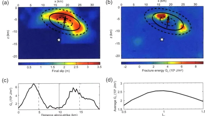
Figure 1. Characteristic rupture ellip
Tottori earthquake (solid black line), r (arrow), centroid location (triangle), and tion (star) plotted on top of slip model of I
seismic gap hypothesis). While both "qu neity" (the asperity model) and "dynam (the seismic gap hypothesis) likely influe individual ruptures to some extent, it is determine which is the dominant behav zones as they have very different implicat term seismic hazard at a particular locatio
25 30 [4] In a given subduction Lone, the trench-normal
con-trols on earthquake rupture are relatively well understood. The fault width is constrained by the updip and downdip limits of the seismogenic zone, at depths of 5 -10 kmn and
25-55 kin, respectively [e.g., Byrne et at., 1988; Pacheco et
aw., 1993; aichelaar and Ruff, 1993; Oeskevich et at., 1999; Lay and Bilek, 2007]. These limits result from transitions
from velocity-strengthening to velocity-weakening behavior
[Schonz, 20021. These transitions likely occur because of
changes in properties such as sediment strength and mineral composition due to changing pressure and temperature conditions [e.g., Byrne et at., 1988; Hyndman and Wang,
1993; Oteskevich et al., 1999].
[5] However, subduction zone earthquakes can release large amounts of seismic moment because extremely long 2.5 3 3.5 fault lengths are possible along a subduction zone. An important question then becomes: what controls the along-se for the 2000 strike limits of these great earthquakes? What stops a
5directivity
M 7.0 earthquake from continuing to rupture along a
upuea subduction zone and becoming a MO 9.0 earthquake? Some hypoceniterenthnngtoveoit-waknngcaavo
vata et a[. [2000]. studies have shown that transverse structures such as ridges
or seamounts in the subducting lithosphere often fragment the subduction zone and may provide natural barriers to enched heteroge- rupture [e.g., Mogi, 1969; Kelleher and McCann, 1976;
;Cloos, 1992; Kodaira et a., 2000, 2002]. However, such
ic hetgnity" structures can also prove to be asperities, as Aberrombie et[
very important to at. [2001] found in the case of the 1994 Java tsunamigenic
ior in subduction earthquake, where the majority of the seismic moment release was centered on a subducted seamount. Therefore ins- the relationship between subducting geological structure and the extent of large individual ruptures remains unclear.
2-4 mHz n 0.5 Model E Data 0 0 90 180 270 360 10-12 mHz 0.5 0 0 1 1 0.5 [ 90 180 270 360 Azimuth 6-8 mHz * 0 E M ilip P' 0 90 180 270 360 14-16 mHz R 0 90 180 270 360 Azimuth
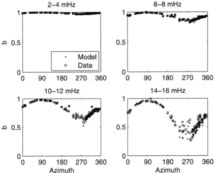
Figure 2. Amplitude measurements (square) and model (circle) from a synthetic line source test at
different frequency bands. The 3-D point source synthetics were used to simulate a 70 km long unilateral rupture propagating to the east with a velocity of 2.5 km/s. Low-amplitude measurements at azimuths of
270 confirm that rupture propagated away from the west. The amplitude anomaly increases with
frequency. In general, the model fits the measurements well at lower frequencies, but at the 14-16 mHz band they begin to differ significantly.
-30'
-60'
60' 90' 120' 150' 180' 210' 240' 270' 300' 330'
Figure 3. Location and focal mechanisms of the 15 M, > 7.5 events in data set.
[6] The upper plate also plays an important role in earthquake rupture. McCaffrey [1993] emphasized the im-portance of fore-arc rheology in seismogenic behavior; strong fore arcs produce more large earthquakes because of their ability to store elastic strain energy. Recent studies
by Song and Simons [2003] and Wells et al. [2003] have
demonstrated that large subduction zone earthquakes occur preferentially in areas along the plate interface which are overlain by fore-arc basins. Song and Simons [2003] found that 80% of the cumulative seismic moment release in the 20th century occurred in the 30% of the total area of subduction zone which exhibited strongly negative gravity anomalies, indicators of the presence of fore-arc basins. Fore-arc basins tend to form in strong, stable wedges and therefore reflect the mechanical and frictional properties along the plate interface over which they lay [Byrne et al.,
1988; Fuller et al., 2006; Wang and Hu, 2006]. To what
extent then can fore-arc structure influence the rupture of individual earthquakes?
[7] This study aims to investigate the relationship between earthquake rupture propagation and fore-arc struc-ture in greater detail. Where do large events start and stop with respect to along-strike structures in the gravity field? To address this question, we estimated the finite source prop-erties of a set of 15 subduction zone thrust events (M, > 7.5)
and compared them to fore-arc structure revealed by maps of trench-parallel gravity anomalies (TPGA) constructed by
Song and Simons [2003]. We find that as a rupture
approaches its eventual extent, the TPGA increases. This correlation, which reinforces the observations of Song and
Simons [2003], suggests that the stress and frictional
heter-ogeneities along the plate interface that control the rupture of large subduction zone earthquakes are expressed in the fore-arc gravity field.
2. Methodology
[8] To evaluate the relationships between fore-arc
struc-ture and individual rupstruc-tures, we require well constrained information on the spatial extent of rupture that can be determined in subduction zones worldwide. This is often a difficult observational problem because most subduction zone ruptures occur offshore and often with limited geodetic and near-field seismic data. Even for the best data sets, detailed finite fault inversions of great subduction zone earthquakes are highly sensitive to model parameterization and station coverage. An example of this is the 2003 Mw 8.3 Tokachi-oki earthquake. Despite the abundance of quality seismic and geodetic data recorded during the event, by far the best data set ever for a M, 8 subduction zone rupture, the finite fault models produced following the earthquake differ in characteristics such as number of asperities and orientation of rupture [Miyazaki et al., 2004a]. Some studies found that the rupture was oriented more along strike of the trench [Yamanaka and Kikuchi, 2003] while others found rupture areas that were half the size and oriented downdip
[Yagi, 2004; Honda et al., 2004; Koketsu et al., 2004; Miyazaki et al., 2004a]. The differences between the slip
models highlight the sensitivity of the results to the different fault parameterizations, constraints, and data sets used in each study. Even for the best combined seismic and geo-detic data sets, the rupture area is only constrained to within a factor of two owing to the limited offshore coverage. Moreover, body wave based studies often have poor con-straints on the seismic moment and slip distribution owing to their relatively high frequency band [Pritchard et al.,
2007].
[9] An alternative approach is to utilize seismic surface waves to constrain only the gross features of the rupture,
Table 1. Characteristic Rupture Dimensions of the Events in This Studya
Event Location M. Lc, km T, s Ivol, kmn/s Directivity Ratio 19920902 Nicaragua 7.6 74 ± 7 40 ± 1 1.8 ± 0.1 0.97 ± 0.10 19940602 Java, Indonesia 7.8 86 ± 7 16 + 2 4.2 ± 1.3 0.78 ± 0.19 19941228 Sanriku-oki, Honshu, Japan 7.7 161 ± 14 20 ± 3 6.1 ± 1.9 0.77 ± 0.16 19950730 Antofagasta, Chile 8.0 121 ± 10 33 ± 1 1.3 ± 0.1 0.35 ± 0.04 19950914 Copala, Mexico 7.3 74 ± 4 14 ± 1 3.2 + 0.3 0.62 ± 0.06 19951009 Jalisco, Mexico 8.0 77 ± 6 32 ± 1 2.1 ± 0.1 0.86 ± 0.08 19951203 Kurile Islands, Russia 7.9 121 9 36 ± 1 1.1 ± 0.1 0.32 ± 0.03 19971205 Kamchatka, Russia 7.8 58 2 34 ± 1 1.6 ± 0.1 0.95 ± 0.02 20010623 Arequipa, Peru 8.4 167 2 27 ± 1 1.1 ± 0.2 0.18 ± 0.02 20030122 Colima, Mexico 7.5 92 6 29 ± 1 1.4 ± 0.1 0.44 ± 0.03 20030925 Tokachi-oki, Hokkaido, Japan 8.3 40 2 45 ± 1 0.9 ± 0.1 0.96 ± 0.02 20031117 Rat Islands, Alaska 7.8 70 21 29 ± 1 2.2 ± 0.4 0.91 ± 0.24 20050328 Sumatra, Indonesia 8.7 137 19 47 ± 3 2.3 ± 0.3 0.79 + 0.15 20060717 Java, Indonesia 7.7 108 5 55 ± 1 1.9 ± 0.1 0.98 ± 0.05 20061115 Kurile Islands, Russia 8.3 93 3 52 ± 1 1.8 ± 0.1 0.98 ± 0.02
aEvent number is date as year, month, day. Errors are ±1 standard deviation. 3 of 31
Table 2. Second Moments Inversion Results" (1,I) (2,0) Earthquake {(02) r 0 ( rr rO rp 00 Op PP Nicaragua 406 23 -11 ±3 374 ±19 615 ±14 6 1 -10 ±6 -18 ±7 423 225 586 131 997 135 Java 65 19 26 4 -70 ±20 262 ±19 56 1 214 46 60 ±17 1514 291 -467 132 1140 170 Sanriku-oki 103 29 4 2 -292 14 -555 18 0.3 0.3 -4 3 -26 ±9 1093 231 990 127 6260 1089 Antofagasta 280 24 22 ± 2 351 14 -53 17 4.7 0.4 48 5 -26 ± 3 1983 272 -1682 271 1963 ± 381 Copala 51 5 -10 1 -145 4 79 4 3.1 0.4 18 4 -44 ±5 601 63 237 43 1311 126 Jalisco 259 10 12 3 -379 14 -373 11 8 1 -15 10 -18 ±9 842 135 686 107 730 109 Kurile 320 18 -28 4 -306 13 164 16 4 1 29 2 -46 ±5 433 124 -434 ±85 3607 ±563 Kamchatka 289 6 -41 2 310 17 -345 16 91 13 9 8 93 ±8 459 42 -363 ±31 486 ±42 Arequipa 187 16 45 5 81 11 187 22 206 ±2 329 16 192 ±45 739 14 -737 ±28 6859 ±177 Colima 210 8 0 4 -264 ±12 129 8 2.0± 0.4 -7 5 -6 ±3 1726 229 717 ±119 725 102 Tokachi-oki 500 10 -2 ±3 -434 ±20 -44 ±8 0.4 ±0.2 2 2 -0.4 ±0.3 406 30 26 ±12 178 32 Rat Islands 208 18 -6 ±3 -59 ±9 -459 ±55 0.8 ±0.1 1 3 12 ±3 151 208 -15 ±305 1228 725 Sumatra 559 ± 73 15 5 1200 42 416 35 2 ± 1 31 11 14 ± 5 4503 1031 -660 ± 581 2117 854 Java 761 ±31 49 5 1022 22 1053 24 5 ±1 65 5 68 ±7 1435 112 1402 ±61 1613 321 Kurile 667 ±12 -50 5 -1077 ±38 472 20 41 ±1 71 7 -31 ±3 1804 106 -788 ±50 431 26
aErrors are ±1 standard deviation. Units of P(0.2) are s2, units off#l"1 are km s, and units of f1( 4" are km2.
such as its extent and directivity. Surface waves have the natural advantages of complete azimuthal coverage and of being inherently low-frequency such that they are sensitive to the entire moment release even for M, 8.5 ruptures. Moreover, properties such as directivity and rupture extent can be estimated independent of any smoothing constraints or other a priori information [McGuire et al., 2001]. We quantify the extent and directivity of large ruptures using the second moments of a scalar source-space-time function describing the moment release distribution [Backus and
Mulcahy, 1976a, 1976b; Backus, 1977a, 1977b; McGuire et al., 2001]. The second moments describe the length,
width and duration of the area of greatest seismic moment release during an earthquake. They are defined as
Ii(2O) = f(r, t)(r - ro)(r - ro)TdVdt (1)
p(0,2) = Jf(r, t)(t - to)2dVdt (2)
t(I.1) = If (r, t)(r - ro)(t - to)dVdt (3)
where f is the source-space-time function and is propor-tional to slip rate at a point on the fault, ro and to are the centroid location and time, #4(2') is the second spatial moment, j(02
) is the second temporal moment, and ftl1) is
the mixed moment which describes overall rupture directivity [McGuire et al., 2001].
[io] The second moments represent weighted averages of seismic moment release, and they define characteristic rupture dimensions that are somewhat smaller than the total rupture dimensions. These characteristic rupture dimensions are [Silver, 1983; Silver and Jordan, 1983; McGuire et al., 2001]
xe(fn) = 2 iT(t(2O)/Mo)n
= 2 (0'2)/Mo
Vo = i , /(02
where Mo is the seismic moment and xc(i) is the characteristic dimension of slip in the direction of i, which has its maximum value of Le when n corresponds to the largest eigenvector associated with the largest eigenvalue of
A2,0). The characteristic duration is -r, the characteristic
velocity is v, and the average velocity of the instantaneous spatial centroid is vo. The velocity v, can range from 1 to 2 times the actual rupture velocity [McGuire et al., 2002]. A directivity ratio is defined by |vol/ve, such that ruptures with directivity ratios <0.5 are predominantly bilateral, while those greater than ~0.5 are predominantly unilateral.
[it] Figure 1 demonstrates the relationship between the characteristic rupture dimensions and the slip distribution of the 2000 western Tottori earthquake. The second moments were calculated directly from the slip model of Iwata et al. [2000]. The ellipse represents the area on the fault plane that released the majority of the seismic moment during the earthquake as measured by the second spatial moment. The arrow indicates the rupture directivity, which is described by the mixed moment.
[12] We estimate the second moments by comparing point
source synthetic and observed seismograms. The data seismogram recorded at station/component p can be expressed as
s,(x, t) =f G (x, x', t - t')Mijf(x', t')dx'dt'
where Mij is the moment tensor, assumed constant during the earthquake, that describes fault orientation; f is the source-space-time function; and GSj is the Green's function.
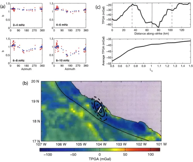
1.5 (a) .o 0.5. 2-4 mHz 0 90 180 270 360 1.5 1 .: *, 0.5 4-6 mHz 0 90 180 270 360 0 20 40 60 80 100 120 Distance along-strike (km) 0 90 180 270 360 Azimuth 0 90 180 270 360 Azimuth 20 N 19 N 18 N 17 N -107 W -100 106 W 105 W 104 W 103 W 102 W 101 W 0 TPGA (mGal)
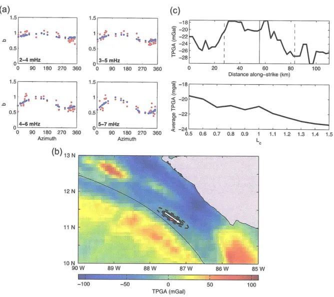
Figure 4. Results for bilateral event 20030122 in Mexico. (a) Amplitude measurements (red) and fit from inversion (blue) at different frequency bands. (b) Centroid (red triangle) and characteristic rupture ellipses with major axes of length 0.5 L, (inner dashed ellipse), 1 L (solid black ellipse) and 1.5 L (outer dashed ellipse) plotted on a TPGA map. Directivity vector vo is shown by the white arrow. The trench is the thin black line. The area of high seismic moment release is largely contained in a negative TPGA region that corresponds with the Manzanillo fore-arc basin. (c) (top) TPGA values in a single profile along strike of the characteristic rupture ellipse. Rupture propagates from the centroid (solid black line) out to both the left and right. Dashed lines mark the extent of the 1 L rupture ellipse. The ends of the plot mark the extent of the 1.5 L, rupture ellipse. (bottom) Average TPGA measured over rupture ellipses of varying L. TPGA is minimized near the centroid (shown by the 0.5 L rupture ellipse). Rupture extent (1 L) corresponds with increasing TPGA.
The Green's function can be expanded in a Taylor series about a point (x'o, t'0):
Gj(x, x', - t') = 1 + (x' -X V + (t' - to)
1 222
-P
G (X, X', t - to') (9)
At low frequencies, the Taylor series can be truncated after the second-order terms allowing the seismogram to be written in terms of the zeroth, first, and second moments:
s,(x,t) = pi'0)GP(x, x'0, t - to)1i + pI
- (x, x,, t - t')ni
+ Pf - G~i (x, x' , t - tol)mii
5 of 31
LLENOS AND MCGUIRE: FORE-ARC STRUCTURE AND GREAT EARTHQUAKES
(a)
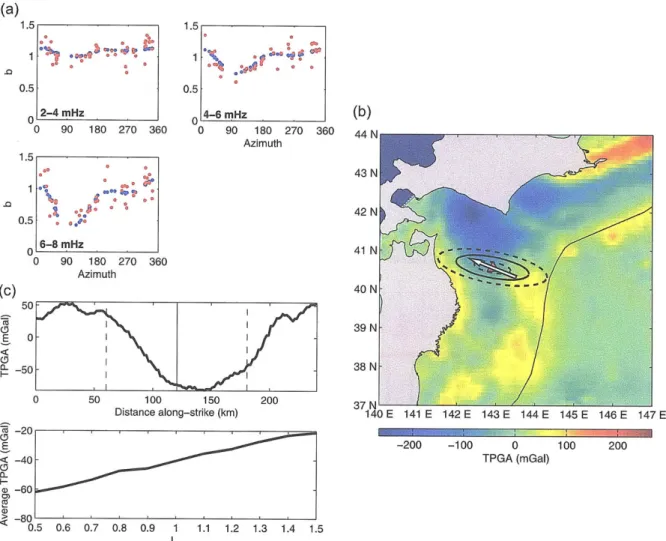
1.5 1 0.5 1-3 mHz 0 90 180 270 360 1.5 1 1 90 180 270 360 Azimuth (b) 7SE 0 90 180 270 Azimuth -23 E -24 (--25 -26 0. 360 0 20 40 60 80 100 120 Distance along-strike (km) 5 0.6 0.7 0.8 0.9 140 160 1 1.1 1.2 1.3 1.4 1.5 105 E 106 E 107 E 108 E 109 E 110 E ll E -250 -200 -150 -100 -50 0 50 TPGA (mGal) 100 150 200Figure 5. Results for unilateral event 20060717 in Java. (a) Amplitude measurements (red) and model
(blue). (b) See Figure 4 for symbol explanation. The area of high seismic moment release shown by the characteristic rupture ellipse (solid black line) stops at a positive TPGA area. (c) (top) TPGA values along strike of the characteristic rupture ellipse. Rupture propagates from left to right. Solid black line denotes the centroid location; dashed lines mark the extent of the 1 L, rupture ellipse, which occurs as the TPGA becomes more positive. The ends of the plot mark the extent of the 1.5 L, rupture ellipse. (bottom) Average TPGA measured over rupture ellipses of varying L,. TPGA is a local minimum at the centroid location (0.5 L).
1 (2) &2
+ p VS Gax ; t-t~
+ p"- sGj (x, x'0 t - tl) Mij
+ : 0 p VssGj(x, x', t -t)i (10)
The first term of the equation on the right-hand side is the point source synthetic seismogram, s, = p0'0)Gi(x, x'0,
t - t'o)Mj. Thus the observed seismogram is described by
the contribution from the best fitting point source perturbed
by finite source effects.
[13] The perturbations to the synthetic seismogram that describe the finite source can be estimated from the data using (10). To measure these anomalies, we rewrite (10) as
sp(x, t) = E m4Ap(t), where m is a vector containing the
independert elements of the zeroth, first, and second moments, and A,,(t) is the partial derivative of the Green's function specific to the ith element of m. Then the cross-correlation function of s and ~,, can be expressed as
Cs (r) = s,(t) ® 3p(t - r) ~ s,(t - r) ( miApi(t) (11) = ms,(t - r) ( A,1(t) 8S 9S 10 S 114 E B09301
c 40-0 30 -, 20 30, 7 7.5 8 8.5 9 Magnitude Mw
Figure 6. Mw versus duration for events in the data set, with a least squares fit showing the scaling between moment and duration. The 1994 Nicaragua and 2006 Java tsunami earthquakes show anomalously long durations for events of their magnitudes.
A system of equations A = b, can then be defined, where the measurement b, is the peak of the cross-correlogram Cs at station p, and Aj is the cross correlation
of A4j(t) with synthetic seismogram s,(t - T). We weight
both b and Aj by the peak of the autocorrelogram of s, to account for arbitrary differences in amplitude between stations. Thus, in our measurement scheme b < 1 implies that the observed seismogram has a lower amplitude than the point source synthetic, as would be expected if the arrival is sensitive to the destructive interference associated with finite source effects in the frequency band being considered. This measurement scheme provides a straight-forward way to identify the directivity of an earthquake. Figure 2 shows the amplitude measurements made from a synthetic line source test simulating rupture propagating toward the east. Low amplitude measurements (b < 1) are
found at azimuths of around 270, away from the direction of propagation.
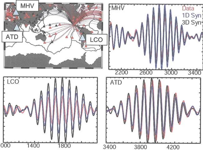
[14] We measured frequency-dependent amplitude anomalies using fundamental mode Rayleigh wave data obtained from the GSN, GEOFON, GEOSCOPE, MEDNET, and China Digital seismic networks through the IRIS Data Management Center. The point source synthetics for an event were generated using the Global centroid moment tensor (CMT) solution for that event, available at http://www. globalcmt.org. We utilized two sets of point source syn-thetics: normal mode synthetics, using the one-dimensional
(1-D) PREM Earth model [Dziewonski and Anderson, 1981] with phase velocity maps correcting for 3-D structure [Ekstrom et al., 1997]; and 3-D synthetics, calculated using
the spectral element method of Komatitsch and Tromp [1999] with the 3-D velocity model CRUST2.0 [Bassin et al., 2000] and mantle velocity model S20RTS [Ritsema and van Heijst, 2000]. We used the 1-D normal mode synthetic seismograms to calculate Apj(t), the partial derivatives of the Green's functions. These derivatives depend primarily on source-station geometry and so the accuracy of the velocity model is
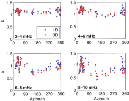
not as important as it is for the amplitude measurements, which we therefore made using the 3-D synthetic seismo-grams. The improvement in Earth model allowed much more accurate amplitude predictions to be made for the Rayleigh wave, especially at the higher-frequency bands used in this study (see Appendix A for further discussion regarding the use of 1-D versus 3-D synthetics).
[15] For each event, we make measurements at a set of global stations with good azimuthal coverage and at a number of frequency bands ranging from 1 to 10 mHz. Waveforms are windowed around the peak of the Rayleigh wave using frequency-dependent window lengths prior to cross correlation. Stations with correlation coefficients less than 0.9 in any frequency band are discarded from all bands in the inversion to avoid errors from unmodeled heteroge-neity. The magnitude of the amplitude anomaly increases with frequency, however, we can only use frequency bands where the amplitude reduction due to finite source effects is less than about 60% of the point source amplitude. Above this band, higher-order terms in (9) become important (Figure 2). The useable frequency range depends on the spatial extent and directivity of the rupture and hence is different for different sized earthquakes.
[16] The inverse problem for the second moments is nonunique but can be stabilized by incorporating the con-straint that the 4-D source region must have a nonnegative volume [Das and Kostrov, 1997; McGuire et al., 2001]. Other constraints are used to limit changes to the centroid depth as well as ensure that rupture does not occur above the Earth's surface. These nonlinear constraints are expressed as linear matrix inequalities in the semidefinite programming approach of Vandenberghe and Boyd [1996]. The least squares objective function (11) is minimized subject to the various inequality constraints. The solution m is a 15 component vector containing the second moments as well as changes to the centroid time, location and seismic moment.
[17] We use a leave-one-out jackknife technique to esti-mate the error of the solution [Tukey, 1984]. We divide the data into N subsets, where N is the number of stations. For the ith subset, the measurements at station i in all frequency bands are left out, and the inversion is performed with the remaining data to produce an estimate of the model param-eters. The N estimates of the model parameters then provide a conservative estimate of the variance of the model parameters [Efron and Stein, 1981]. The variance of the model parameters can then be used in standard error propagation equations to estimate the variance in derived quantities such as Le and TC [Bevington and Robinson, 1992].
[is] The characteristic rupture ellipses for each event are compared to the maps of trench- parallel gravity anomaly
(TPGA) produced by Song and Simons [2003]. To construct
these maps, an average trench normal gravity profile for each subduction zone is removed from the free air gravity
data [Sandwell and Smith, 1997] along the length of the
subduction zone. The resulting TPGA illuminates shorter-wavelength features such as fore-arc basins. We compare the characteristic rupture dimensions with the spatial varia-tions in TPGA to test the hypothesis that a correlation exists between variations in the TPGA field and earthquake
of 31
LLENOS AND MCGUIRE: FORE-ARC STRUCTURE AND GREAT EARTHQUAKES 1.5 0.5 1 2-4 mHz 0 90 180 270 360 1.5 0.5 * 6-8 mHz 0 0 90 180 270 360 Azimuth
(b)
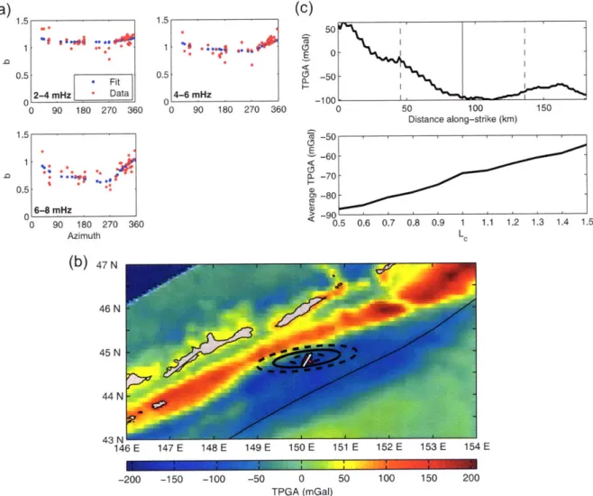
0 90 180 270 360 Azimuth 21 S 22 S 23 S 24S 25 S 26S 27S 28S 0 50 100 150 Distance along-strike (km) 40 0 E 31 0) a. .25 0.5 0.6 0.7 0.8 0.9 1 1.1 1.2 1.3 1.4 1.5Figure 7. Results for event 19950730 in Chile. (a) Amplitude measurements (red) and model (blue).
(b) See Figure 4 for symbol explanation. Although the majority of the seismic moment released in this
event occurred in a high TPGA region, the centroid is located in a local TPGA minimum. (c) (top) TPGA values along strike of the characteristic rupture ellipse. Rupture propagates from the centroid (black line) out to the limits of the rupture ellipse (dashed line). The ends of the plot mark the extent of the 1.5 Le rupture ellipse. TPGA values at along-strike distances of less than 50 km should be ignored because they
occur inland, where the TPGA measurements are not as accurate. (bottom) Average TPGA measured over rupture ellipses of varying L,. Inland TPGA values were masked out in calculating the average. Again a local minimum occurs near the centroid.
rupture characteristics such as centroid location, rupture extent and directivity.
3. Results
[19] We estimated the second moments for 15 shallow
thrust earthquakes (M, > 7.5) that occurred on the plate
interface in circum-Pacific subduction zones from 1992 to
2006 (Figure 3). Because of the complex nature of the
moment release during the 2004 Sumatra earthquake, this event was not included in our analysis. Table 1 summarizes the characteristic rupture dimensions of these events and Table 2 summarizes the second moment inversion results. Several representative events are discussed in greater detail below. Appendix B contains our Rayleigh wave measure-ments and comparisons with the TPGA field for each event.
3.1. The 2003 Colima Mexico Earthquake
[20] On 22 January 2003, a M, 7.5 earthquake occurred near the state of Colima, Mexico. This event primarily ruptured bilaterally in the updip-downdip directions [Yagi
et al., 2004]. Our second moment estimates (Table 1 and
Figure 4a) support this conclusion. The inversion resulted in a characteristic rupture length Le of 92 km, a duration re, of 29 s, and a directivity ratio of 0.44. This agrees well with
the finite source model determined by Yagi et al. [2004] using a joint inversion of teleseismic body wave and strong motion data.
[21] The characteristic rupture ellipse representing the area of greatest moment release is compared to the TPGA field in Figure 4b. Although the measurements and direc-tivity clearly indicate a downdip rupture, the ellipse is oriented more along strike. The centroid is located in a