A constrained optimization approach to control with application to flexible structures

A Constrained Optimization Approach to Control

with Application to Flexible Structures

by

Lawrence Kent McGovern

SUBMITTED TO THE DEPARTMENT OF AERONAUTICS AND ASTRONAUTICS

IN PARTIAL FULFILLMENT OF THE REQUIREMENTS FOR THE DEGREE OF

Master of Science

Massachusetts Institute of Technology

©

The author hereby grants to MIT permission to reproduce and to distribute copies of this thesis document in whole or in part.

Signature of Author D

Department of 'eronautic and Astronautics May 10, 1996

Certified by

Dr. i'ret D"Appleby Charles Stark Draper Laboratory Thesis Supervisor

Certified by

Professor Steven R. Hall Department of Aeronautics and Astronautics

SThesis Advisor

Accepted by

. Professor Harold Y. Wachman

,,ASSACHUSETTS INSTI.lt, _{' 'irmdn, Departmental Graduate Committee}

OF TECHNOLOGY

JUN

11

1996

_Aero

A Constrained Optimization Approach to Control

with Application to Flexible Structures

by

Lawrence Kent McGovern

Submitted to the Department of Aeronautics and Astronautics on May 10, 1996 in partial fulfillment of the

requirements for the degree of Master of Science

Abstract

A controller design methodology which minimizes a linear or quadratic closed-loop design metric subject to a set of linear design specifications is presented in this thesis. Several useful convex design specifications in the time and frequency domain are given, and posed as sets of linear constraints on the closed loop. The use of these constraints is demonstrated in the context of a simple magnetic bearing control example.

The closed-loop optimization relies on a finite-dimensional approximation of the achieveable space of closed-loop transfer functions. Previous work of this nature has favored a finite impulse response (FIR) approximation. Alternative sets of or-thonormal basis functions are explored which can lead to more efficient closed loop approximations than the FIR filter.

The constrained optimization method was applied to an active vibration isolation system. The complete controller designs and hardware test results are presented. Due to an abundance of closely-spaced, lightly-damped structural modes, controller design for the active vibration isolation system proved to be a formidable task, in which an efficient formulation of the basis functions became essential. The controllers were designed by directly constraining the closed loop to meet a set of performance and robustness constraints.

Thesis Supervisor: Dr. Brent D. Appleby Title: Senior Member of the Technical Staff Thesis Advisor: Professor Steven R. Hall

Acknowledgements

A large part of the credit for the success of this thesis belongs to my thesis supervisor, Dr. Brent Appleby. Due to his impressive "sixth sense" for control theory, I have never felt at a loss for ideas worth pursuing. I am indebted to the countless hours he has

spent discussing the course of this thesis with me. He is also one of the nicest guys to have as a supervisor, which made this experience all the more rewarding.

I am also grateful to Tim Henderson, who provided the practical application for this research, and gave me the freedom to try new and non-standard methods of control design on this system. I feel very fortunate for the opportunity to ground my research in a real hardware system.

I thank Prof. Steven Hall for many useful and interesting discussions over the past year. His suggestions have been very valuable to the development of this thesis.

Nicola Elia certainly deserves a big thanks, as does Dr. Rami Mangoubi. They have each offered my invaluable help in understanding the f1 control theory, which was the foundation of most of my research.

Finally, I would like to extend my warmest thanks to Ellen Block. Her continual love and support has always brought out the best in me. Thank you!

This thesis was prepared at The Charles Stark Draper Laboratory, Inc., under Contract 6-2872-60321. Publication of this thesis does not constitute approval by Draper or the sponsoring agency of the findings or conclusions contained herein. It is published for the exchange and stimulation of ideas. I hereby assign my copyright of this thesis to The Charles Stark Draper Laboratory, Inc., Cambridge, Massachusetts.

Contents

2.3 Small Gain Theorem . . . . 2.4 Parameterization of All Stabilizing Controllers 2.5 Rational Matrix Factorization . . . .

3 Controller Synthesis in the Time Domain

3.1 Performance Objectives . . . .. 3.1.1 3W2 Optimization ...

3.1.2 fl Optimization ...

3.2 Feasibility Constraints . . . . 3.2.1 Zero Interpolation Conditions . . . . . 3.2.2 Rank Interpolation Conditions . . . . . 3.2.3 Delay Augmentation Method . . . . . 3.3 Solution to the fl and l12 Problems . . . . 3.4 Optimization in Q-space ... 13 . . . . . . . . .. . . . . . 13 . . . . . . . . . . . 16 . . . . . . . . . . . .. . 17 .. . . . . . 18 19 19 20 22 22 24 27 . . . . . 27 . . . . 28 . . . . 28 . . . . . . 29 . . . . . 30 . . . . . 32 .. . . . . 33 . . . . . 34 . . . . 37

4 Linear Design Specifications 4.1 Time-Domain Constraints ... 4.1.1 Example ... 4.2 Frequency-Domain Constraints 4.2.1 Example ... 4.3 Stability Margin ... 4.4 Robust Stability... 4.4.1 Example ...

4.5 Linear Matrix Inequalities . . .

39 . . . . 4 0 . . . . 4 0 . . . . . 4 3 . . . . . 4 5 . . . . 4 6 . . . . . . . .. . 4 8 . . . . 4 9 . . . . . . . . . . 5 2

5 Efficient Basis Functions for Closed Loop Approximations

5.1 Fixed Pole Model... ... . . ... 5.2 Laguerre Functions ... ...

5.3 General Orthonormal Basis Functions . . . . 5.4 Basis Functions in the Constrained Optimization Control Problem

5.4.1 Performance Objective Functions 5.4.2

5.4.3

Time-Domain Constraints . . . . Frequency-Domain Constraints . . . . . . ...

6 Application of Constrained Optimization Methods to an Active Vi-bration Isolation System

6.1 Structural Test Model . . . . 6.2 Design Objectives . . . .. 6.3 Phase One Design . . . .. 6.3.1 Optimization . . . . 6.3.2 Choice of Basis . . . . 6.3.3 Performance Specifications . 6.3.4 Stability Robustness . . . . 6.3.5 Controller Reduction . . . . 6.3.6 Experimental Results . . . .

6.4 Phase Two Design . . . .

55 56 60 63 67 . . . . . 6 7 69 69 71 . . . . . 72 . . . . . 74 . . . . . 76 . . . . . 77 . . . . . 78 . . . . . 79 . . . . . 80 . . . . . 81 . . . . . 83 . . . . . 86

6.4.1 6.4.2 6.4.3 6.4.4 Performance Specifications . . . . . . . . .. Stability Robustness .. ... Controller Reduction . . . . . . . . . .. Experimental Results . . . . 87 87 89 91 7 Conclusions 95

7.1 Recommendations for Future Work . ... 97

List of Figures

2.1 Feedback connection for Small Gain Theorem . ... 2.2 Closed-loop system augmented with stable Q...

4.1 Disturbance profile ...

4.2 Response to fixed input for design with time-domain constraints . 4.3 Frequency response for design with frequency-domain constraints. 4.4 Response to fixed input for frequency-domain constrained design. 4.5 Minimum distance d from Nyquist plot to critical point ...

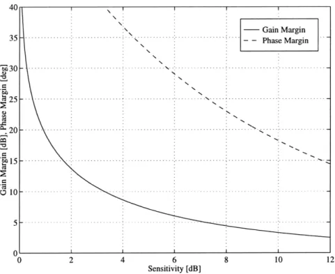
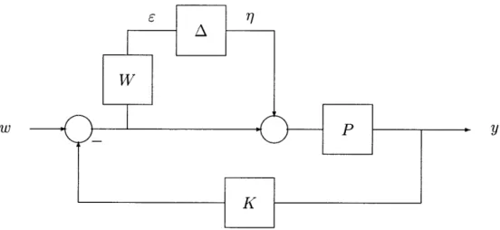
4.6 Gain and Phase Margins versus Sensitivity Magnitude... 4.7 Feedback control with multiplicative uncertainty . ... 4.8 Condensed loop with uncertainty ...

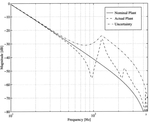
4.9 Uncertainty for plant with structural modes . ...

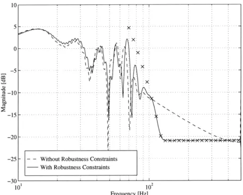
4.10 Frequency response of PK/(1 + PK) for design with robustness con-straints...

4.11 Magnitude constraint approximated with 8 linear constraints. 4.12 Magnitude constraint posed exactly as an LMI ...

5.1 5.2 5.3 5.4 5.5 5.6 5.7

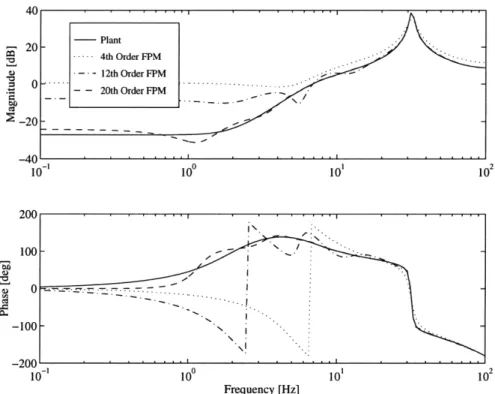
Fixed-Pole Model approximation of H(z) . . . . .

Coefficients 0n for a 20th order FPM . . . . .

Impulse response of H(z) ...

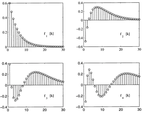
First four Laguerre functions for a = 0.8 . . . . . 1IH

-OTF112 as a function of a for first example . . . . .

Comparison of 50 state Laguerre model and FIR model..

IIH - _OTF112 as a function of a for second example. . . .

. . . . . 58 . . . . . 59 ... . 59 . . . . . 61 . . . . . 63 . . . . . 64 . . . . . 65

6.1 Structural Test Model. ... . . ... .. 73

6.2 Disturbance force PSD ... 75

6.3 Strut 1 open loop and closed loop using the classical controller. ... 76

6.4 Comparison of linear model and FRF data for phase 1 design .... 77

6.5 AVIS disturbance rejection problem. . . . .. . . . .... 78

6.6 Impulse response of the closed loop using the classical controller. . . . 79

6.7 Constrained optimization and classical performance for phase 1 design. 80 6.8 Two previous AVIS controller design, and resulting frequency constraints. 82 6.9 Constrained complementary sensitivity of the phase 1 design... 82

6.10 Controller reduction for phase 1 design. . ... 84

6.11 Wavefront error PSD performance for phase 1 design. . ... . 85

6.12 Image motion performance for phase 1 design. . ... 85

6.13 Reduced design model. . ... ... 87

6.14 Constrained optimization and classical performance. . ... 88

6.15 Complementary sensitivity of phase 2 design. . ... 89

6.16 Sensitivity of phase 2 design. . ... .... 90

6.17 Nichols plot with linear model of design with stability margin constraints. 90 6.18 Nichols plot with FRF data of classical and constrained optimization designs. ... ... 91

6.19 Controller reduction for phase 2 design. . ... 92

6.20 Effect of controller reduction on closed loop. . ... 92

6.21 Wavefront error PSD performance for phase 2 design. . ... 93

Chapter 1

Introduction

1.1

Motivation

As described by Boyd and Barratt [1], the fundamental problem of control engineering is to find a controller for a given system that meets a set of design specifications, or to determine that no such controller exists. This problem is so far unanswered by current methods of controller design. Traditional methods are often the most indirect in addressing this problem, but they are also the methods which have the widest experience base. The current state of computer technology, along with advances in optimization techniques, offers the possibility for much more direct methods to address this problem.

The techniques of classical control engineering are well established, and have been successfully used for many decades. These techniques include root-locus methods, Nyquist diagrams, Nichols charts, and varying degrees of reasoning and intuition by the engineer. However, there are many drawbacks to classical methods of control design. These methods are geared towards single-input/single-output (SISO) systems, and often have trouble with multiple-input/multiple-output (MIMO) systems with large amounts of cross coupling. Classical methods also do not address optimization. It is up to the designer to iterate until an acceptable design is found. Finally, classical methods can be very indirect at dealing with particular design specifications. Often, it is difficult to understand exactly how a design must be changed to improve the

overall performance.

Modern controller design methods provide an analytic solution to certain classes of control problems, such as the Linear Quadratic Gaussian (LQG) control problem [18]. These methods are based on a state-space representation of the system, and can easily handle MIMO problems. In the LQG framework, a cost functional is chosen to reflect the cost of error in the regulated output and of actuator use. Optimization of this cost leads to a constant state feedback matrix. A Kalman filter is then used to estimate the plant states, based on a Gaussian white noise model of plant disturbances and sensor noise. This leads to the optimal controller design as long as the model is perfect, the plant noises are correctly modeled, and the cost functional has been correctly determined. However, rarely does a control problem correctly fit into the LQG framework. More often, the control engineer uses the cost and noise weights as parameters to "tweak" a design until it has the desired properties. Robustness can be added by shaping the loop gain with frequency weights on the cost functional, by adding fictitious noise, or through the use of the Loop Transfer Recovery (LTR) method [18]. In the end, the standard method is often abandoned, and the desired controller is derived in an indirect way.

The question naturally arises whether there is a more direct method of controller design. There are a multitude of design specifications which may be placed on a closed-loop system. A few examples are maximum overshoot due to a particular input, the frequency response in a particular frequency band, or stability robustness for a set of model uncertainties. While some analytic methods have successfully integrated common design specifications into the solution (e.g., l7- theory addresses the issue of robust control), the majority of control problems with design specifications do not have a known closed-form solution. This does not prevent these problems from being solved by means of brute force optimization. However, these problems are infinite dimensional and frequently are non-convex, meaning they may have many local minima. To be made tractable, the problem must be approximated in a finite number of dimensions (e.g., approximating a transfer function as a finite impulse response (FIR)). Even with this approximation, determining the global minimum of

a non-convex optimization problems with a reasonable amount of computations can be done only for small problems.

Convexity is therefore a very important characteristic of optimization problems. If the objective function and the set of design specifications are convex, then any local minimum is guaranteed to be the global minimum. This means that the convex opti-mization problem can be solved much more efficiently than the non-convex case. In [1], Boyd and Barratt show that a large number of design specifications can be posed as convex constraints on the closed loop. By only considering convex constraints, they have also shown that it is possible to efficiently determine the limits of performance achieved by any linear time-invariant (LTI) controller for an LTI system, subject to the finite dimensional approximation. This is a powerful tool for the control engineer, because it determines if a set of design specifications are overly stringent.

One of the most celebrated convex optimization routines is the Simplex Method [6], which efficiently solves the following problem:

min cT x xERn

subject to

Aex = be

Ax < bi

A problem in this form is known as a linear program. Closely related is the quadratic

program, which includes in the objective function a quadratic term, xTGx. If the

constant matrix G is positive definite, then the objective function is convex. A convex quadratic program also may be solved efficiently [14]. If possible, it is advantageous to formulate convex optimization problems as linear or quadratic programs. Because of their extreme efficiency, these are the optimization methods explored in this thesis. It will become clear in later chapters that many design specifications can be posed as or approximated with a set of linear design specifications.

1.2

Historical Background

In the 1960s, Fegley and colleagues published a series of papers noting the usefulness of linear and quadratic programming to the design of control systems [12]. Using these methods, they were able to find an optimal controller subject to a set of linear constraints by solving for the coefficients of the closed-loop FIR. Their examples used only simple SISO systems, and their ideas were not extended to more complicated systems, but part of this is presumably due to the state of computer technology at the time. The approach that Fegley and his colleagues outlined was an insightful way of incorporating a variety of convex constraints into the controller design process. The basis of this method, linear and quadratic programming, is of practical use today due to vastly improved computer speeds and optimization methods.

Linear programming became central to the solution of the f1 optimal control problem by Dahleh and Pearson in 1987 [7]. The goal of the f1 control problem is to minimize the maximum peak-to-peak gain of a closed-loop system driven by an unknown but bounded disturbance. The solution to this problem was found to be the solution of a finite-dimensional linear program. There is a striking similarity between the solution to this problem, and the types of problems being solved by Fegley. For the optimal f1 solution, Dahleh and Pearson proved that the closed loop has an FIR structure, so the solution was formulated in terms of the closed-loop impulse response. This formulation makes the addition of linear design specifications very straightforward, but addition of these constraints was not explored until later [8].

Convex optimization in control system design was revisited by Boyd and col-leagues in 1988 [2]. This paper describes a controller design method based on a software program called QDES developed by the authors. In this approach, the emphasis was placed on optimization over the free parameter Q in the well known

Q-parameterization [20]. The closed loop is affine in

Q,

New methods of convex optimization are beginning to take hold in the control community. Following recent advances in interior-point convex optimization algo-rithms by Nesterov and Nemirovskii [19], many more types of convex constraints may be accommodated efficiently in convex optimization programs. Linear and quadratic programming are limited to linear constraints. The interior-point methods proposed by Nesterov and Nemirovskii can accommodate linear matrix inequality (LMI) con-straints. These methods are currently finding practical applications in the field of control [3, 4, 5].

1.3

Contributions

The most significant contribution of this thesis is a complete design of a linear con-troller, tested on a real hardware system. This lends credibility to the field of convex optimization as a practical tool for controller design. In demonstrating a new control method, academic examples are often used which have been developed specifically for the control theory they are demonstrating. By using a real world control ex-ample, the method must instead be tailored to the example. In the literature, the academic examples used to demonstrate constrained optimization almost universally rely on an FIR model of the closed loop. In practice, this is often not an efficient representation of a transfer function (i.e., thousands of terms may be required in the FIR). Therefore, this thesis expands an existing constrained optimization method to accommodate other basis functions. Another contribution to the method is a more general way of posing constraints on the closed-loop frequency response when the de-lay augmentation method is used. It will be seen in that under certain conditions, the delay augmentation method can invalidate constraints on the closed loop. A solution to this problem for frequency constraints is presented in this thesis.

1.4

Organization

This thesis focuses primarily on optimization directly in the closed-loop space using linear and quadratic programming, and neither the method used in QDES nor the use of LMIs are explored in detail. These methods are worth noting because of their close relationship with the methods used in this thesis. The methods which are used are closely based on the methods developed by Dahleh and Diaz-Bobillo [8].

The organization of this thesis falls into seven chapters. The second chapter con-sists of necessary background material. Chapter 3 approximates the closed loop as an FIR filter, and develops the closed-loop optimization as a linear program for £1 op-timization, and a quadratic program for 12 optimization. Optimization in Q-space rather than directly in the closed-loop space is mentioned in the final section, but does not play a significant role in the thesis. The design specifications are incorpo-rated into the design in Chapter 4. This chapter is concerned primarily with linear constraints, because they can easily be appended to a linear or quadratic program. LMI constraints are briefly discussed at the end of this chapter, but the use of LMI constraints is left for future research. Chapter 5 explores the use of basis functions other than the FIR which may approximate the closed loop more efficiently than the FIR. Chapter 6 presents a complete controller design using constrained optimization methods for an active vibration isolation system. The controllers designed for this system were successfully implemented on a hardware testbed. Finally, the conclusions and suggestions for further research are presented in Chapter 7.

Chapter 2

Background

This chapter presents a brief overview of some well-known concepts necessary for the development of this thesis. It should serve as an aid to understanding the concepts and notation used in later chapters. Therefore, the reader may safely skip this chapter if the concepts are already familiar, and refer back to it as needed.

2.1

Signal Norms

The size of a signal can be measured by the calculation of one of its norms. The p-norm of an n-dimensional discrete signal x[k] is defined as

||x| = EE |xi [k] I

P

k=0 i=1 I

When the p-norm of a signal is bounded, the signal exists in the space that will be useful to this chapter are when p = 1, 2, oc.

Perhaps the most widely used norm is the f2 norm of a signal.

defined by (2.1) ,p. The norms This norm is 1 IIx12 = x z[k]x[k]

The £2 norm corresponds to the total amount of energy contained in a signal. Also related is the average power of a persistent signal (with infinite energy). This is also known as the root-mean-square (RMS) of the signal. Technically not a norm, the

RMS of a signal is defined as

1

|I X|rms lim n - E x[k]Tx[k] .

N-o N k=0

For signals with large variations in amplitude, the RMS value may not be adequate as a measurement. In this case, it may be better to look at the fo norm,

||x|ll = max sup wi [k]|.

i _k

The foo norm therefore represents the peak value the signal attains. This norm is useful to describe an unknown but bounded input signal, and to describe the maximum level achieved by an output signal.

The £1 norm is important as a measurement of total resource consumption, e.g., if the signal magnitude represents the amount of fuel used per unit time. It is also an important measurement of a system impulse response, as will be discussed in the next section. The £l norm is defined as

n oo

11x -= E E Ixik]f

i=1 k=O

2.2

System Norms

Systems are generally measured in terms of the norms of the input and output. One system measurement which will be important to this thesis is the average power output to a stochastic stationary input. For a MIMO system H with dimension nz x

nw, and an input with power spectral density S,,(ei0_{), the output can be measured}

as

jHw rms = Tr H(eio)Sww(eiO)H(eio)*dO . (2.2)

If the input is unit variance white noise, then IIHWj rms is known as the 72 norm of the system H, written IIHll2. In this case, Sw(eo) = I, and by Parseval's theorem,

Equation 2.2 becomes

00

/

IIH 2 = Tr E H[k]H[k] = EZZ hj4 [k]

2 _(2.3)

where H[k] is the matrix impulse response of H with components hi [k]. Thus, the

W₂ norm of a system represents the RMS output given a white noise input, and can

be determined by measuring the the £2 norm of its output given a unit impulse input. The .oo norm of a system is an induced norm, defined as

|Hw|

IHIOo

This norm is the maximum £2/£2 system gain, and can be calculated by finding the supremum of the maximum singular values over all frequencies, i.e., IH11 0 = sup, r(H(eiwT)).

The final system measurement which will be important to this thesis is the induced norm

IIHII1

This is the peak gain of the system over all possible bounded inputs, and can be found by calculating the £1 norm of the system impulse response. To understand why the f4 norm provides an upper bound on the system gain, consider a SISO system h. Given an exogenous input with a known bound in magnitude

|w||oo

output will be bounded by

lz||oo = sup 1 h[k - j]w[j]

k j=0O

00

< Z |h[k]| = |hll.

k=0

Therefore the system will have a bounded output if and only if the system pulse response h E f1, and the induced ,oo norm of h will be bounded by its fl norm.

This guarantee can easily be extended to the MIMO case. Given the system

H

C

guaranteed to be bounded by

1t1l0

Figure 2.1: Feedback connection for Small Gain Theorem.

2.3

Small Gain Theorem

Figure 2.1 illustrates a feedback system between two systems, H1 and H2. The

sta-bility of this closed-loop system depends on the stasta-bility of the transfer function

(I - H1H2)- 1. If both H1 and H2 are stable, then as long as the gain of H1H2 is

less than unity at all frequencies (i.e., |IHIH2 11 < 1), the closed loop is guaranteed to be stable. This is known as the Small Gain Theorem [9]. The Small Gain The-orem is not a necessary condition for stability, but is a good robustness condition if the phase of one of the transfer functions is unknown. An even more conservative test for stability can be applied if only the W-o norms of the systems are known. Because ||HllooflH 2 0. >

IH

2.4

Parameterization of All Stabilizing Controllers

The standard control problem consists of a plant P which maps exogenous input

w and control input u to the regulated output z and measurement y. A feedback

compensator K then closes the loop from the measurement to the control input. The plant can be represented by

z P11 P12 W

Y P21 P22 U The closed loop transfer function is

where .F(P, K) denotes the lower linear fractional transformation.

An important restriction on K is that it must be internally stabilizing. To satisfy the internal stability requirement, f(P, K) can be replaced by the well-known

Q-parameterization

Pd = T1 + T2QT3 (2.4)

in which Q must be stable, but is otherwise arbitrary [18, 20], and T1, T2, and T3 are

described below. This parameterization has two advantages over the parameterization

..F(P, K). First, the search space over all stabilizing controllers is replaced by a search

over all stable Q. Secondly, the parameterization in Equation 2.4 is affine in

Q,

A Q-parameterization can be derived from any nominally stabilizing controller. If the plant P has the state space description

x[k+1] = Ax[k] + Blw[k]+B u[k]2

z[k] = Clx[k] + Dow[k] + D12u[k]

y[k] = C2x[k] + D21w[k] + D22u[k]

then a stabilizing model-based controller can be constructed by choosing a controller gain matrix F and an observer gain matrix H such that all the eigenvalues of A - B2F

and A - HC2 are inside the unit circle. Let , denote the states of the model-based

controller. Adding an input v and an output e to the controller, where u = -Fi + v

and e = C2(x - 2), the model-based controller can be augmented with any stable

system v = Qe without affecting the stability of the closed-loop system. Figure 2.2 illustrates the augmented closed loop. For this system it can be shown that the transfer function from v to e is zero, so Q affects the closed-loop system only in the forward loop. This results in the affine representation in Equation 2.4, where

T, = Transfer function from w to z of nominal closed-loop system T2 = Transfer function from w to e

Figure 2.2: Closed-loop system augmented with stable Q.

The state space representation for the augmented controller K. is

,[k + 1] = (A - B2F - HC 2 + HD 22F),[k] + Hy[k] + (B2 - HD22)v[k]

u[k] = -Fi[k] +v[k]

e[k] = -(C 2 - D22F)[k] + y[k] - D22v[k].

The space of all stabilizing controllers is spanned by K = Ye(K, Q) such that Q is stable. Notice that when the open-loop plant is stable, the controller and observer gain matrices in K, can go to zero. This reduces the Q-parameterization to T = P11, T2 = P1 2, and T3 = P2 1.

2.5

Rational Matrix Factorization

In Section 3.2, it will be necessary to use a well-known rational matrix factorization, the Smith-McMillan decomposition [18]. This factorization is defined in this section, as applied to a rational MIMO system. It is useful for characterizing the zeros in a MIMO system, which in addition to a complex number, also have a direction associ-ated with them. The Smith-McMillan decomposition of an n x m system G(z) with

rank r is found by factoring G(z) into

G(z) = L(z)M(z)R(z)

where L(z) and R(z) have full rank independent of z, and

M(z) = E,(z) l1(Z) ,r(Z) V)r(Z) 0 0

is an m x n matrix in Smith-McMillan form. The polynomials ce(z) and 'i(z) are coprime for each i, and satisfy the following divisibility property: Ci divides ei+1 without remainder, and 4i+l divides

'i

l

U

multiplicity of each zero zo in ej(z) as ai(zo). Then the total multiplicity of a zero in

Chapter 3

Controller Synthesis in the Time

Domain

For many types of control engineering problems, closed-loop optimization in the time domain provides a distinct advantage over the standard frequency domain techniques. Many specifications given for a closed-loop system are placed on the magnitude of the output signals based on a characteristic input signal. Common examples are peak overshoot to a step input, rise and settling time, or maximum output to an unknown but bounded input. In addition, specifications given in the frequency domain can also be placed in the time domain, such as the output amplitude to a sinusoidal input. If the closed-loop optimization is in the time domain, consideration of time domain specifications become much more straightforward. This chapter presents a control design algorithm which models the closed loop as a finite impulse response (FIR). Most of this methodology is based on the £1 design algorithm developed by Dahleh and Diaz-Bobillo [8].

3.1

Performance Objectives

The optimality of a feedback controller requires that a particular performance metric of the closed-loop system is optimal, e.g. minimized. Section 2.2 covered several system norms which provide a way to measure the performance of a controller design.

This section shows the objectives of the 7-2 and eL control problems in terms of the closed-loop impulse response.

3.1.1 712 Optimization

If the disturbance entering a system is unknown but has a known Gaussian power spectral density, then a shaping filter can be appended to the input to create a new system with a white noise input. When the input disturbance is a unit variance white noise, it is often desirable to minimize the amount of power seen at the output due to the disturbance. This is equivalent to minimizing the expected value of the output 2-norm, E(||Z112), which in turn is the 7-2 norm of the closed-loop system. From

Equation 2.3, the 'H₂ minimization problem can be stated as

/

fz flw 00

JR2 opt = inf 1H1| = inf C hij[k]2 . (3.1)

i=1 jl=1 k=0

Frequency-domain weights are an effective tool for forcing the optimization to concentrate on a particular frequency band while placing less emphasis on other bands. This is done by minimizing the '-2 norm of an appended system IWH11₂,

where W is a stable filter. The weighted 12 optimization problem is then

, nz w 00

J2 opt = inf (i * hij) [k]2 _(3.2)

i=1 j=1 k=O

where wi[k] is the impulse response of the frequency weight on output i.

3.1.2

f1 Optimization

When the probabilistic nature of a disturbance is unknown, but the signal is known to be bounded in magnitude, i.e. Iwlloo 1, then the performance of the closed-loop system can be measured by considering the maximum possible magnitude of the regulated output,

IIlzllo.

Jt opt = inf

IH

h

3.2

Feasibility Constraints

From Section 2.4, all achievable closed-loop transfer functions are represented by the Q-parameterization

H = {T1 + T2QT3 I Q stable}. (3.4)

For this problem formulation, it is desirable to find the constraints on the impulse response h such that H can be written in the form of Equation 3.4. There are two important sets of conditions placed on the transfer function R = T2QT3 which

guarantee that H is feasible. The first set of conditions is that the non-minimum phase zeros of T2 and T3 must be preserved in R to guarantee the stability of Q. These

constraints are known as the the zero interpolation conditions. If the problem is one-block, meaning there are the same number of measurements as disturbances and the same number of controls as regulated outputs, then the zero interpolation conditions are the only feasibility constraints. If the problem is not one-block, then Q has limited degrees of freedom. There may be fewer measurements than disturbances (ny < n,), or there may be fewer controls than regulated outputs (nu < nz). Individually both

of these cases are called two-block problems. If both n, < nw and n, < nz, then

the problem is considered four-block. This places a limitation on the structure of R, which has dimension nz x nw, while Q only has dimension n, x ny. The conditions to ensure this are the rank interpolation conditions.

This section shows that it is possible to pose these conditions as linear constraints on the impulse response, but does not explicitly show how these constraints should be calculated in practice. The methods used in this section rely on the Smith-McMillan decomposition of certain transfer matrices, which can present numerical difficulties when implemented on a digital computer. A numerically stable method for construct-ing the interpolation conditions which circumvents the Smith-McMillan decomposi-tion can be found in [10].

3.2.1

Zero Interpolation Conditions

It is easiest to understand the motivation behind the zero interpolation conditions by considering a SISO example, where h(z) = ti(z) + t2(z)q(z). If r(z) = t2(z)q(z),

then the condition that r(z) must satisfy to insure that h(z) is feasible is that q(z) =

r(z)/t 2(z) must be stable. This means that any non-minimum phase zero z0o in t2(z)

must also be present in r(z), i.e., r(zo) = 0. This imposes the constraint on h(z), that

h(zo) = tl (zo). If the non-minimum phase zero has multiplicity a, then this condition

must also be placed on the first a - 1 derivatives. Therefore, ( )(zo) = (d n t (zo)

for n = 0,..., (a- 1).

The MIMO case is not as simple, and it is helpful to use the Smith-McMillan decomposition of the transfer matrices T2 and T3, as developed in Section 2.5:

T2 = LT₂ MT₂ RT T3 = LT3 MT3RT3 where Enu MT2 nU 0 ... 0 00 ... 0 0 ... 0 MT 3 "'. "

The zero interpolation conditions will now be stated without proof. (A proof and more complete treatment of the following result can be found in [8].) Define

R = T2QT3. If ci and e have a non-minimum phase zero z0o of multiplicity ai(zo)

and Ua(z 0), then the (i,j) entry of the matrix ( d - LL RR )(zo) must also be zero

condition, define the following row and column vectors:

ai(z) (LT)(i,:)(z) i = 1, 2, ..., nz (3.5)

3(z) = (R )(:,j)(z) j = 1, 2,...,nw

where the indicial notation T(i,:) denotes the ith row of matrix T and T(:,j) denotes the

jth column of matrix T. Now the zero interpolation condition for each non-minimum phase zero can be written as

(

n

= 0,...

. ai (Zo)

+

u'(Zo) - 1

It is now important to show that these condition can be written as set of lin-ear constraints on the closed-loop impulse response hij[k]. Because R = H - T,

Equation 3.6 can be rewritten as

d" d"

dz (aiHj) (zo) = dz (aiT, j)(zo) (3.7)

The product aiHj is equivalent to

(aiHj )(zo) = Tr[H3ja i](zo)

nz nw = E (Hpq/qjYip)(Zo) p=l q= nz nw 00 = E E (~jp/qj)(zo)hpq[k]z0k p=l q=1 k=0

This can be substituted back into Equation 3.7 to obtain

d n nw 00 dn

dzn (E E E ipqjhpq[k]z-k) dzn (iT )(zo) (3.8)

p=1 q=1 k=0 Z=ZO dZ

The zero interpolation constraints are now written as a set of linear constraints on the closed-loop impulse response hij[k]. It is useful to vectorize this impulse response as

h -_ [hll[0] - hlnw[0] h21[0] --- h2nw [0].-- hnzn. [0] hil[l] " ' ]T. (3.9)

With this definition, it is possible to rearrange the zero interpolation conditions in Equation 3.8 into a single linear operation:

3.2.2

Rank Interpolation Conditions

The rank interpolation conditions preserve the structure of R = T2QT3 if the problem

is multiblock (two or four-block). From the Smith-McMillan decomposition of T2 and T3 introduced in the previous section, the ith row of MT2 is zero for n, < i < nz, and the jth column of MT3 is zero for ny < j < nw. This means that the ith row

of (L21R)(z) should equal zero for nu < i < nz, and the jth column of (RR')(z)

should equal zero for ny < j < n,,. Using the definitions of a and 3 in Equation 3.5, these conditions can be stated as

(aiR)(z) = 0 for i = n + 1,...,nz (3.10)

(RP)(z) = 0 for j= n + 1,..., n

By transforming from the z to the time domain, the rank interpolation conditions appear as an infinite number of constraints on the impulse response of R, r, [k]:

ap[k- l]rp[1] = 0 for q ,...,n (3.11) p=1 l=0 k 0 nw k j = nu + l ' nw ) 1 q[ k - 1]rp[1] = 0 for p = 1,..., nz q=1 l=0 k > 0

Then, by replacing rij[k] with hij[k] - (T1)ij[k], the zero interpolation conditions

become a set of linear constraints on hij[k] and can be written in the following form:

Arankh =

brank-Notice that the constraints in Equation 3.11 are over all k > 0, which leads to an infinite number of constraints. Therefore, the range of Arank is infinite. This leads to practical difficulties when trying to impose these constraints using a computer. This problem is resolved in the next section, by means of the delay augmentation

method. This method approximates the multiblock problem with a one block problem,

3.2.3

Delay Augmentation Method

The delay augmentation method was developed by Diaz-Bobillo in [10] as a method for approximating a multiblock problem as a one block problem. In doing this, the need for rank interpolation conditions is avoided, and only a finite number of inter-polation constraints are needed to solve the problem. In preparation for the delay augmentation method, the general multiblock closed-loop system must be partitioned as follows:

H11 H12

T

+

where the dimensions of T2,1 and T3,1 are n, x n, and n, x ny. To transform this into a one-block problem, the parameter Q must have dimensions nz x nw. To achieve this, Q is augmented with extra parameters, and T2 and T3 are augmented with N

pure delays:

H,N H12,N T1,11 T1,1 2 T2,1 0 Q11 Q12 3,1 T3,2

H21,N H22,N T₁,2 1 T1,2 2 T2,2 SN Q21 Q22 0 SN

(3.13)

where SN = Iz - N is the system of appended delays.

The system HN is now one-block, and inf IIHN| can be solved without any rank interpolation conditions. Of course, Q12, Q21, and Q22 are not present in the real system, and can be used as extra degrees of freedom in the optimal solution to Equa-tion 3.13. Therefore, inf IHN provides a lower bound to the optimal solution of Equation 3.12. That is,

inf IIHN| 1< inf IIHN| = inf ||HI|. (3.14)

Q stable Q1 1 stable Q11 stable

Q12=Q21=Q22=0

Also, an upper bound on the optimal solution is obtained by using the Q11 from the optimal solution to Equation 3.13, and setting the rest of the parameters to zero so the solution is feasible. For the fl control problem, it was proven in [10] that as N -+ , the lower and upper bounds converge on the optimal solution. It is assumed here that the 7-2 control problem should show similar behavior. This convergence can be seen

intuitively by considering the expansion of Equation 3.13: HN = T1 + T2Q1 1T3 + SNRN (3.15) where 0 T2,1Q 12 RN = Q2 1T3,1 Q21T3,2 + T2,2Q12 + SNQ22

Notice that the H11,N partition is unaffected by the parameters Q12, Q21, and Q22.

Also, these extra parameters will not affect any partition of HN [k] for k < N due to the time delay in SNRN appearing in Equation 3.15. Therefore, the augmented parameters in Q have a decreasing effect on the closed loop as the augmented time delay is increased.

As a final point on the delay augmentation method, it should be noted that while there are no longer an infinite number of rank interpolation conditions, there are extra zero interpolation conditions due to the introduction of delays in T2 and T3. Because an Nth order delay has the transfer function z- N, there are also N

non-minimum phase zeros at infinity. These zeros must be accounted for in the interpolation conditions to guarantee that Q will be causal.

3.3

Solution to the £1 and 7-12 Problems

The f1 design problem can be easily posed as a linear program. Because of the nonlinearity (the absolute value) in Equation 3.3, a change of variables is necessary. Let hij[k] = h+[k] - hj[k], where h+ [k] > 0 and h [k] > 0. While this definition does not restrict h+[k] or h-[k] to be zero depending on the sign of hij[k], the magnitude

of h can be found by

|hij[k] = min (h+ [k] + h[k]). h+ [k],h- [k] j

Using this notation, define the objective function as

nw oo

p = max E (h [k] + h [k]).

It should be understood that p is not necessarily the lI norm of H. However, when f is minimized, either hj[k] or h- [k] will be zero for every (i, j, k). In this case, it is evident that p will be the el-norm of H. Therefore, the optimal (minimum) l1-norm

of the closed loop has the property |HII1 optimal = infP.

Next, using the vectorized closed-loop impulse response h defined in Equation 3.9, define the linear operator At, such that

nw oo

(A, h)i = E E hij[k] for i = 1,...,

nz.

j=1 k=0

Then the objective function is written as

p = max(A 1 (h' + h-))i.

The problem can now be posed as a linear program:

IH 1 optimal inf _, p,h+,h -subject to (3.16) h+ [At, At,] h- 1

h-Azero -Azero h+ bzero

Arank -Arank h- brank

[h+ _{h-]T > 0}

where 1 is a vector of ones with dimension n,.

Similarly, the 7-2 design problem can be posed as a convex quadratic program.

Using the vector representation of the MIMO impulse response in Equation 3.9, the

W2 norm becomes hTh. If there are frequency weights, then the 7-2 norm is instead

hTh = (w * h)T(w * h). The weighted impulse response h can be constructed as

follows:

h[O] w[O] 0 0 ... h[0]

h[1] w[1] w[O] 0 ... h[1] h[2] w[2] w[1] w[O] ... h[2]

Therefore h = Wh where W is a matrix operator, and the objective function is simply

the quadratic hTWTWh. The quadratic program takes the form

IIH 2 optimal = inf hTWTWh

h

subject to (3.17)

Azeroh bzero

Arankh = brank.

Immediately it should be recognized that neither Equation 3.16 nor Equation 3.17 are practical to solve. There are infinitely many variables, due to the infinite dimen-sion of h. Additionally, if the problem is multiblock, there are also infinitely many constraints from the infinite range of Arank. However, an approximate solution is within the reach of a computer. As was seen in Section 3.2.3, the delay augmentation method can be used to reduce the infinite number of constraints with a finite number of constraints. Alternative methods to delay augmentation also exist, and can be found in [8].

The infinite dimension of h can be reduced to a finite dimension by assuming that

hi,[k] = 0 for k > N, where N is a finite number of time steps. In fact, it can be proven using Duality Theory that this is in fact the case for the one-block fl control problem. This proof appears in [8]. Unfortunately, there is no equivalent guarantee for the f- 2 optimal solution. However, it is not unreasonable to approximate the terms

in the impulse response after a certain time as zero, because the impulse response of an W₂ optimal solution will be stable, and therefore will have an exponential decay

towards zero.

Once the l1 and F2 problems are approximated as finite dimensional linear and quadratic programs, they can be readily solved using standard techniques. The Simplex Method still proves to be the most effective method for solving linear pro-grams, by searching for the optimal solution along the constraint boundaries [6]. The quadratic program can also be efficiently solved if the quadratic objective function is convex, which will be the case as long as the matrix WTW is positive definite. This problem can be solved using the methods in [14].

3.4

Optimization in Q-space

In Section 2.4, it was noted that the Q-parameterization is affine in Q, meaning that if Q1 and Q2 each yield a feasible closed loop, then so does AQ1 + (1 - A)Q2 for every A E R. This useful result does not hold for a parameterization that is made in the closed loop space. Just because H1 and H2 are achievable does not imply

that AH1 + (1 - A)H2 will be achievable. However, the space of all achievable closed

loops is convex, meaning that feasibility is guaranteed if A E [0, 1]. Thus the closed-loop representation used in this chapter (its impulse response) must be used with a set of convex specifications to insure feasibility. These are the feasibility constraints introduced in Section 3.2.

It follows that if the closed loop is represented as a linear combination of stable Q transfer matrices, that there will no longer be a need for feasibility constraints. That is, represent H with a set of variables x E RN with

N

H = T + T2

Z

n=l

where {Qn} is a sequence of stable transfer matrices. This is exactly the approxima-tion used by Boyd and his colleagues in [2]. This paper describes a software package they have developed, called QDES, which approximates Q as an FIR filter as follows:

Qijk(Z) = Eijz-k_{, 1 < < n, < j < ny, < k < N,}

where Eij is a matrix with the (i, j) entry as one and all the others zero.

The use of the approximation in Equation 3.18 is not explored further in this the-sis, but would be worthwhile to compare with the other techniques presented in this chapter. Optimization in Q-space does offer several advantages over optimization in the closed-loop space. Removing the need for feasibility conditions reduces the com-plexity of the problem, especially for multiblock problems. Also, the optimization is only over the number of transfer functions in Q rather than the number of trans-fer functions in H, which may have many more inputs and outputs. However, the optimization problem is still inherently infinite dimensional. Because this problem must be reduced to a finite dimensional subspace, the subspace cannot be chosen

arbitrarily. It was not clear what the best subspace in Q would be, although an FIR basis would certainly not be a bad start. It is left as an open question whether it is more effective to solve for the closed loop in terms of Q or to solve directly in the closed-loop space.

Chapter 4

Linear Design Specifications

The amount of computation required to find the solution to a constrained optimization problem can be greatly improved if the constraints are known to be convex. In a convex optimization problem, once a local minimum is found, it is guaranteed to be the global minimum. This is one reason why the Q-parameterization introduced in Section 2.4 is significant. This parameterization is affine in Q, and the space of all stable Q yields the space of all feasible closed-loop transfer functions. Thus the most important design specification, feasibility, is also convex. An extensive treatment of

the various kinds of closed-loop convex constraints is given in [1].

This chapter will focus on a particular subset of convex design constraints, namely linear constraints. Often, a set of convex constraints can be reasonably approximated with a finite set of linear constraints. For example, it was seen in Section 3.2 that feasibility can be approximated with a set of linear constraints. Linearity allowed the feasibility constraints to be written in the framework of a linear program for the f1 control problem, and a quadratic program for the 7-2 control problem. Both of these techniques converge on an answer much more rapidly than other techniques which can handle non-convex constraints. Most controller design problems will have additional design specifications beyond feasibility, many of which are convex. This chapter will present several typical design specifications that are often used, and show in detail how they can be posed as linear constraints.

4.1

Time-Domain Constraints

In Chapter 3, the closed loop was optimized in terms of its impulse response. This formulation makes it very convenient to introduce constraints on the closed loop in the time domain. A constraint on the impulse response at a particular time has the form gi[k] < hij[k] < gu[k] where gl[k] and g,[k] are the lower and upper bounds. In engineering practice, it is often more useful to look at the step response of a closed-loop system. Typical examples of step response specifications are overshoot and undershoot, asymptotic tracking, rise time and settling time. The step response can easily be derived by integrating the impulse response, and is therefore available to constrain [8]. In fact, the response to any particular fixed input wj can be constrained in the same way, and is found by taking the convolution zi = hij * wj. In order to put

the time domain constraints into a useful form, they must be written as

Atimeh < btime, (4.1)

where h is defined in Equation 3.9. Equation 4.1 can then be appended to the linear and quadratic programs developed in Section 3.3.

It should be noted that if a problem is multiblock and the delay augmentation method is implemented, once the extra parameters in Q are thrown away the time domain constraints may no longer be satisfied in the solution. If the constraints were placed on H11, then the constraints will still be satisfied. This is because the extra

parameters in Q do not affect the first block. However, if the constraints were placed on the H12, H21, or H22 blocks, then the constraints are guaranteed to be satisfied

only for times less than the number of delays used. The reader should refer back to Section 3.2.3 for a more detailed explanation.

4.1.1

Example

Magnetic bearing control in aircraft engines provides an excellent example of the use of time-domain constraints. Magnetic bearings offer potential advantages to aircraft engine technology by allowing the rotor shaft to spin in a virtually frictionless envi-ronment. An important design requirement on the magnetic bearing controller is that

2000 B 1500 1000 500 0--500 -1000 0 1 2 3 4 5 6 Time [sec]

Figure 4.1: Disturbance profile.

it should not allow the shaft to come into contact with the bearing walls under normal operating conditions. This event is most likely to happen as a transient response to an aircraft maneuver. This problem therefore has hard constraints on the amplitude

of the output due to a specific disturbance input.

The shaft position in the magnetic bearing has two degrees of freedom which are assumed to be uncoupled for this example. The system inputs are the control and disturbance forces, and the output is the position. The rigid-body dynamics for one axis can therefore be modeled as a double integrator. With a 0.001 sec time step, the plant dynamics are represented in discrete time as

z2

y(z) = 3.667 x 10-3 _{(W(Z)+ u(z))}

( Z - 1)2

where the input is in units of pounds and the output is in mils.

The most extreme disturbance that may occur during a maneuver is shown in Figure 4.1. This disturbance profile is based on an aircraft maneuver which produces an 11g acceleration at the bearing. Under these conditions, the maximum allowable deflection of the shaft is 6 mils.

0

-

-

-8-0 0.5 1 1.5 2 2.5 3 3.5 4 4.5 5 Time [sec]

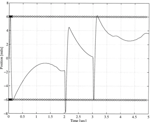
Figure 4.2: Response to fixed input for design with time-domain constraints.

This problem was solved as an iW2 minimization problem. Although Chapter 3 developed the solution to this problem using an FIR basis, hundreds of terms in the FIR would have been required to reach a feasible solution, and thousands required to reach the desirable one. As will be seen in Chapter 5, the 72 problem is not restricted to using the FIR basis, and another more efficient basis set was chosen for the solution. A Laguerre basis (see Section 5.2) with a time scale of 0.9 and 120 free coefficients was chosen. Both the position output and control effort were weighted in the objective function. Unity scalar weights were placed on both position and control. Time-domain constraints were then placed on the output due to the disturbance in Figure 4.1, restricting the output to be between +6 and -6 mils.

The resulting transient is shown in Figure 4.2. Note that at 2 seconds, the signal actually violates the constraints. Closer inspection of the plot will show that the signal actually crept between two discrete time domain constraints (the x's), so technically no constraint was violated. This shows a limitations of this method, which can only handle constraints at a finite number of points.

4.2

Frequency-Domain Constraints

Design specifications are frequently placed on the magnitude of an output due to a persistent sinusoidal input at a particular frequency. Consider the bound in magni-tude on the SISO system H:

IH(ei<

)I

This bound in magnitude is equivalent to the constraint

R~[H(ei"T)] cos 0 + .[H(ei"T)] sin - 7 VO E [0, 27).

In [8], this constraint is approximated by a finite number of linear constraints on the real and imaginary parts of H(eiwT) by only considering a discrete number of angles

0 evenly spaced between 0 and 27. In turn, the real and imaginary parts of H(eiwT)

are linear functions of h[k]:

00

R[H(eiwT) = h[k] cos(kwT)

k=0

![H(eiwT)] = -

Z

k=0

Finally, the frequency constraint can be written as

o00

E h[k] cos(kwT + 0,) 7y where 0, = {2n/N I n = 0, 1,..., N - 1}. (4.2)

k=0

The frequency domain constraints are guaranteed to be satisfied if the problem is one-block. If the problem is multiblock, and the delay augmentation method is used, then only the constraints placed in the first block, H11, are guaranteed to be met. This

is due to the introduction of the extra free parameters, Q12, Q21, and Q22, which are not present in the actual system. If frequency constraints are required on an input-output pair that is not in the H11 block, then these constraints should be reflected

onto the H11 block. Consider the constraint H(i,j)(eiwT) 7y, where H(i,j) represents

the SISO transfer function from input j to output i, and the input-output pair (i, j) does not exist in the H11 block. This new notation is introduced to prevent confusion

with the notation Hij, which represents the ij partition and is not necessarily SISO. As before, an equivalent constraint is R~[H(i,j)(eiwT)] cos 0 + Q[H(i,j)(eiwT)] sin 7 y.