The State of the Art in Multilayer Network Visualization

HAL Id: hal-01944505

https://hal.archives-ouvertes.fr/hal-01944505v2

Submitted on 8 Feb 2019

HAL is a multi-disciplinary open access

archive for the deposit and dissemination of

sci-entific research documents, whether they are

pub-lished or not. The documents may come from

L’archive ouverte pluridisciplinaire HAL, est

destinée au dépôt et à la diffusion de documents

scientifiques de niveau recherche, publiés ou non,

émanant des établissements d’enseignement et de

The State of the Art in Multilayer Network

Visualization

Fintan Mcgee, Mohammad Ghoniem, Guy Melançon, Benoit Otjacques,

Bruno Pinaud

To cite this version:

Fintan Mcgee, Mohammad Ghoniem, Guy Melançon, Benoit Otjacques, Bruno Pinaud. The State

of the Art in Multilayer Network Visualization. Computer Graphics Forum, Wiley, 2019, 38 (6),

pp.125–149. �10.1111/cgf.13610�. �hal-01944505v2�

The State of the Art in Multilayer Network Visualization

Fintan McGee

, Mohammd Ghoniem

Guy Melançon

, Benoit Otjacques

, and Bruno Pinaud

1

_{Luxembourg Institute of Science and Technology (LIST),}

firstname.lastname@list.lu

2

_{University of Bordeaux, LaBRI UMR CNRS 5800, France}

firstname.lastname@u-bordeaux.fr

February 8, 2019

Abstract

Modelling relationships between entities in real-world systems with a simple graph is a standard approach. However, reality is better embraced as several inter-dependent subsystems (or layers). Recently the con-cept of a multilayer network model has emerged from the field of complex systems. This model can be ap-plied to a wide range of real-world datasets. Exam-ples of multilayer networks can be found in the do-mains of life sciences, sociology, digital humanities and more. Within the domain of graph visualization there are many systems which visualize datasets hav-ing many characteristics of multilayer graphs. This report provides a state of the art and a structured analysis of contemporary multilayer network visual-ization, not only for researchers in visualvisual-ization, but also for those who aim to visualize multilayer net-works in the domain of complex systems, as well as those developing systems across application domains. We have explored the visualization literature to sur-vey visualization techniques suitable for multilayer graph visualization, as well as tools, tasks, and an-alytic techniques from within application domains. This report also identifies the outstanding challenges for multilayer graph visualization and suggests future research directions for addressing them.

1

Introduction

Simple graphs are often used to model relationships between entities in real-world systems. This ap-proach may however be an oversimplification of a much more complex reality better embraced as sev-eral interdependent subsystems (or layers), which motivated the development of the complex networks field [43, 68]. The concept of a multilayer net-work [73] builds on and encompasses many exist-ing network definitions across many fields, some of which are much older, e.g., from the domain of soci-ology [19, 91, 123].

As an introductory illustrative example, consider a person’s social networks. People frequently use more than one social network platform, e.g., Facebook for their personal social network or LinkedIn for their professional. Offline, "real life", social networks could also be considered, again with relations being either personal or professional. These networks can be sidered independent, however they can also be con-sidered as layers in a multilayer graph. The networks overlap as some people may be present across layers. Layers are in this case characterised by relationship type (either online/offline and personal/professional). A significant change in one network may implicitly correlate with or cause changes in another. For ex-ample, a change of employer will cause changes in both offline and online professional networks but in a different manner for each, and may cause slower,

more gradual, changes in the personal offline/online social networks. To answer some questions, it may be necessary to also include employers or companies as entities of the network. This makes it possible to model explicitly person-company relationships, as well as person-person and company-company rela-tionships. In this case, layers may be characterised by entity type (either person or company). Other definitions of layers are also possible as illustrated in Section 2.

Examples of multilayer networks can be found in the domains of biology (the so-called “omics” lay-ers), epidemiology [94,107,125], sociology (in a broad sense, including fields such as criminology, for in-stance) [17, 19, 28, 32, 40, 44, 46, 80], digital human-ities [37, 89, 114], civil infrastructure [22, 31, 35] and more. Multilayer networks have been explicitly recog-nised as promising for biological analysis [49]. We give more details in Section 2.4.

In the area of network visualization many sys-tems visualize datasets having many characteristics of multilayer networks, albeit under a different ti-tle. Multi-label, multi-edge, multi-relational, mul-tiplex [22, 102], heterogeneous [37, 108], and multi-modal [46, 55], multiple edge set networks [28], in-terdependent networks [43], interconnected networks [107] and networks of networks [68] are amongst the many names given to various types of data that are encapsulated by the Multilayer Networks definition of Kivelä et al. [73].

Recently initial steps have been made towards con-solidating the work on visualization of multilayer net-works from domains outside of the information visu-alization field, see MuxVis [30] from the domain of complex systems, or from the domain of social net-works [33], based on the complex systems paper of Rossi and Magnani [104]. However, to date there has been no survey quantifying and consolidating the state of the art of visualization of multilayer net-works, both within the field of information visual-ization and across application domains.

The goal of this survey is to reconcile the many vi-sualization approaches from the information visual-ization field and the application domains and group them together as a consistent set of techniques to support the increasing demand for the visualization

of multilayer networks. The final contribution of this work consists in identifying the key challenges out-standing in the field, and providing a road map for future research developments on the topic.

This report is structured as follows: Section 2 presents the defining concepts underlying multilayer graph models, and points out the main differences they have with other related network models. The rest of the section briefly describes the application domains in which multilayer graphs are encountered. The description of the methodology followed is pre-sented in Section 3 followed in Section 4 by the survey itself. It provides a structured account of relevant tasks, visualization and interaction techniques per-taining to multilayer network analysis. In Section 5 we reflect on the state of the art in multilayer net-work visualization, and point out open challenges and opportunities that lie ahead of the information visu-alization research community. We finish this paper in Section 6 with concluding remarks and a roadmap for future contributions to the topic of multilayer net-works visualization.

2

Multilayer Networks and

Re-lated Concepts

The notion of many relationships between individ-uals, often called multiplex relationships, is semi-nal in sociology and one could argue that it al-ready was present in the sociograms introduced by Moreno [91]. The notion is central in the work of Burt and Schøtt [19] where the challenge is to some-how simplify multiplex relationships, consolidate and substitute them for relationships involving a smaller number of relation types to ease the analysis of the network. More recently, the concept of a multilayer network has emerged from the Complex Networks area, a subdomain of the field of complex systems, and is a fertile ground for novel visualization research.

2.1

Defining concepts

It is important to emphasise that layers do not re-duce to some operational apparatus. The concept

goes far beyond a simple intent to capture data het-erogeneity. While it is true this notion is most of the time embodied as nodes and edges of a network being of different “types”, its roots lie deeply in sociol-ogy [19, 44, 80]. This notion is used to form questions and hypotheses, where layers can be considered as innermost, intermediate or outer [85]. For instance, Dunbar et al. [36] consider networks similar to our introductory example, and examine to what extent online and offline layers in personal networks over-lap.

While innermost and outermost layers are well es-tablished notions in sociology, the modeller is free to be “creative” when deciding what constitutes a layer (dixit Kivelä et al. [73]). That is, the notion of a layer in a network emerges from and belongs to the domain under investigation. Consequently, when discussing the notion of layer, it is important to distinguish the sociological network from the mathematical network used to describe it. The mathematical network – a graph – is but an artefact through which we may hope to observe and ultimately characterise a phenomenon occurring on the sociological network. The definition of a layer is thus a characteristic of the multilayer sys-tem as a whole, defined either by a physical reality or the system being modelled. The notion of a layer naturally occurs when describing tasks performed by analysts; it can be mobilised to form exploration or browsing strategies (see Section 4.1).

Formal Definition. A standard graph is often de-scribed by a tuple G = (V, E) where V defines a set of vertices and E defines a set of edges (vertex pairs), such that E ⊆ V × V . An intuitive defini-tion of a multilayer network first consists in specify-ing which layers nodes belong to. Because we allow a node v ∈ V to be part of some layers and not to others, we may consider ‘multilayer graph’ nodes as pairs VM ⊆ V × L where L is the set of considered layers. Edges EM ⊆ VM × VM then connect pairs (v, l), (v0, l0). An edge is often said to be intra or inter -layer depending on whether l = l0 or l 6= l0.

Going back to the example where people use different social network platforms, we would have L = {l, l0, l00, . . .} where l = Facebook friends, l0 =

LinkedIn connections, l00 = “real life” family-friends-acquaintances, etc.

2.2

Aspects

Kivelä et al. also define what they call aspects as a way to characterise a set of elementary layers relating to some concepts. An example would be:

• aspect L1 capturing interaction between people in the context of their participation to events (e.g., conferences [5]), with l1for interaction dur-ing InfoVis, l2 for interaction during EuroVis, etc.);

• aspect L2 capturing co-authorship around themes (an example we borrow from Renoust et al. [102]), with li for co-authorship associated with some keyword ki;

• aspect L3 capturing project partnership, with layers li associated with specific programs, for example [46];

• and so forth.

Aspects can also be used as an artefact to deal with time or geographical position.

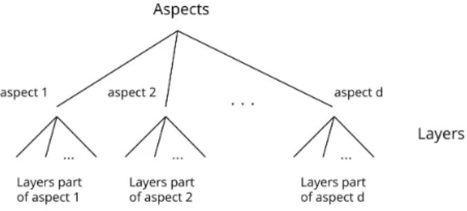
Figure 1: Aspects can be seen as groups of layers of different types. Nodes do not necessarily appear on all layers, but they necessarily appear on at least one layer of each aspect.

Aspects can be captured by extending the previous definition, as proposed Kivelä et al.:

Given any number d of aspects, L = {L1, L2, . . . , Ld}, a multilayer network corre-sponds to a quadruple M = (VM, EM, V, L), where

each aspect La is a set of elementary layers and VM ⊆ V × L1× . . . Ld. That is, while nodes do not necessarily appear on all elementary layers, they nec-essarily appear on at least one layer of each aspect. The set of edges of M simply is EM ⊆ VM× VM (see Figure 1).

Kivelä et al. chose the term carefully, to avoid using a term that may be unclear depending on the reader’s domain. While the term dimension, in its lit-eral meaning, may lend itself to the concept of defin-ing a characteristic, aspect has been chosen due to the use of the term dimension as jargon in different domains.

Another example lies in the domain of biology (de-scribed further in Section 2.4). One aspect is the type of data, such as genomic, metabolomic or proteomic. Another aspect might be the species, or different bi-ological pathways, as illustrated in Figure 2. If the biological data contains time information, that may also be considered an aspect. While multiple aspects are a possibility for multilayer network data sets, it is not a requirement. A multilayer data set may be defined by a single aspect, which categorises multi-ple layers. See Table 1 for a sammulti-ple list of aspects and layers extracted from the literature surveyed as part of this report. Kivelä et al. [73] provide further examples in their extensive list of multiplex datasets and their associated layers.

Incidentally, Wehmuth et al. [128] propose an alter-native definition they call MultiAspect graphs where they formally define what can be considered as an as-pect. Unsurprisingly, they also form a network where nodes are defined using Cartesian products collect-ing multiple values into a scollect-ingle entity. The authors describe MultiAspect graphs as forming a generali-sation of Kivelä et al.’s multilayer network. Recon-ciling these different approaches is beyond the scope of this paper. Well developed examples are certainly needed to uncover the full applicative potential of MultiAspect graphs.

2.3

Related Graph Models

Below, we review related graph models (see also Fig-ure 3) and their differences or resemblances to multi-layer networks.

Figure 2: A purely illustrative example of multilayer data in the context of biology. The layer can be de-scribed by the type of data as a first aspect (genomic, proteomic, or metabolomic), and biological pathway being represented as second aspect.

2.3.1 N-partite Graphs

Recall that a bipartite graph is made of two disjoint sets of vertices so that no two vertices belonging to the same set are connected. Bipartite graphs can be considered as a case of multilayer networks with 2 layers and only interlayer edges. The two mode (i.e., node type) nature of bipartite graphs result in analytics that are different to those of single mode graphs [11]. Bipartite graph concepts are sometimes extended into n-partite graphs, as seen in our exam-ple in figure 3a, although in practice many of the 2 mode restrictions associated with bipartite graph are not fully retained. In practice, systems which model bipartite cases and extensions of bipartite cases, such as the multimodal networks of Ghani et al. [46], and the Academic network analysed by Shi et al. [113], can be considered instances of multilayer networks. In this case the authors also make use of bipartite analytics (e.g., adapted centrality metrics) to better understand their network structure.

Bipartite networks can be reduced to single mode networks via projection on a mode. Such an

opera-Aspect Description Layer Definition Source Paper Source Paper Domain Social entity type People, societies / organisations [102] Information visualization Social relationship type Friendship, aggression [28] Social networks

Word relationship Hyponym, homonym [54] Information visualization Year of publication [1974...2004] [54] Information visualization

Infrastructure

connection type Air connection, train connection [53] Physics

Transport mode air, rail, ferry, coach [42] Scientific data (Transportation) “Omics” Entity type Gene, protein, protein structure [95] Biology

Historical correspondences

Letter, letter sender,

letter receiver, cited book [121] Historical network research Building layout Arrangement of house spaces [115] Robot Control Algorithms

Table 1: Examples of aspects and layers, extracted from papers covered by this survey.

(a) An n-partite graph (n = 3).

Node 1 Type: A Value1: 0.2 Value2: 17 Value3: "High" Node 2 Type: A Value1: 0.4 Value2: 11 Value3: "Med" Node 3 Type: C Value1: 0.25 Value2: 22 Value3: "High" Node 4 Type: B Value1: 0.9 Value2: 17 Value3: "Low" Node 5 Type: B Value1: 0.8 Value2: 16 Value3: "High" Node 6 Type: C Value1: 0.9 Value2: 10 Value3: "Low" Node 7 Type: A Value1: 0.05 Value2: 1 Value3: "High" Node 8 Type: B Value1: 0.15 Value2: 30 Value3: "Med"

(b) A Multivariate graph, where each data node contains multiple attributes.

T =1 T =2

T =3 T =4

(c) A dynamic graph, with 4 time slices, where structure changes over time.

Figure 3: Illustrative examples of related graph models: Each of the three nodes types (*indicated by colour) of the n-partite graph could define a layer within a multilayer network, in this case all edges would be between layers. For a multivariate graph, node attributes could be used do divide the network into layers. Defining layers by node type in this example would result in three layers, although that may not make sense for the system being modelled, as there would be no edges within the layers of nodes of type B and C. For a dynamics graph characterized by time slices, each time slice can be intuitively understood as a layer. Further insight could be gained by by the use of an additional aspect to define layers.

tion may be used to also define a layer in a multilayer network, if the projection results in a layer that re-flects the reality of the system being modelled.

2.3.2 Multivariate Graphs

Multivariate graphs [71] are those in which nodes or edges carry attributes or properties. As described by

Schreiber et al. [108], there is a relationship between multivariate graphs and multilayer graphs. Some variables or attributes in a multivariate dataset often serve the purpose of distinguishing nodes and edges that belong to different layers, e.g., the type of so-cial network platform in our initial example. There are also multivariate visualization applications such as that of Pretorius and van Wijk [97], that define

their graph as having discrete sets, which can be con-sidered analogous to defining layers. However, in the majority of cases research into multivariate visualiza-tion lacks the a priori definivisualiza-tion of a layer defined by a physical or conceptual reality related to the system being modelled.

In faceted datasets, multivariate data items are grouped in multiple orthogonal categories. Originally used as an approach to search and browse large data stores and text corpora [21, 116], later work extended the faceted approach to include relationship visual-ization [83, 134]. Datasets can have many different facets such as spatial and temporal frames of refer-ence, or multiple values per data item and as such can be considered multifaceted. Visualizations for multi-faceted data are those which show more than one of these facets simultaneously (see Hadlak et al. [52] for a survey of multifaceted graph visualization tech-niques). Hadlak et al. discuss primarily four com-mon facets of network structure considered in net-work visualization, and their composition: partitions, attributes, time, and space. These facets may be con-sidered to be very similar to instances of Kivelä et al.’s aspects. However, they can be considered as dif-ferent ways of exploring a single data set, (which is unsurprising given the origins of a faceted visualiza-tion). The techniques described are still very useful for developing approaches for visualizing layers, par-ticularly where the layer type matches the Hadlak et al.’s selected faceted categories. However faceted network visualization approaches do not meet all the needs for multilayer network visualization. While multilayer networks may use notions similar to these facets to characterise layers, multilayer network vi-sualization also focuses on the interactions between layers and the role of layers in the network as a whole.

2.3.3 Dynamic Graphs

Dynamic graphs are graphs whose structure (nodes and edges) and/or associated attributes may change over time. Analysts are often interested in comparing the state of the network at different points in time. Within the domain of complex networks Boccaletti et al. [10] consider the dynamics of multilayer net-works, and in many cases time slices of a dynamic

(or temporal) network are simply mapped to layers. The notion of dynamic networks is also mentioned by Kivelä et al., who notes that they can be considered as a type of multilayer network. A set of dynamic time slices can be considered layers in an aspect rep-resenting time. As multilayer networks can have mul-tiple aspects, a temporal aspects might be just one of many. In their report on dynamic network visual-ization Moody et al. [90] explain the importance of “multiplicity” in social networks, i.e., the overlap of types of relations. In particular, they point out that linking relational timing to tie types allow to better investigate social dynamics. A recent survey of dy-namics graph visualization techniques was provided by Beck et al. [7], but does not consider layers in any context other than a hierarchical graph.

2.4

Application Domains and Data

Across all of the application domains described in Section 1, advances in sensors, scientific equipment, and technology mean that researchers have access to more data than ever. This wealth of complex data is often best understood as a multilayer network model.

Life Sciences: Within biological network visual-ization there are many contexts in which a multi-layer network approach may be beneficial [49]. Bi-ologists have access to more genomic, proteomic and metabolomic data, allowing for the construc-tion of complex multilayer models of intricate bio-logical processes. Interactions taking place within the genomic, proteomic and metabolomic levels can be modelled as individual networks, but interactions also occur between elements sitting in different omics levels within a larger biological system, where the as-pect characterising the layer is the node type [26]. This corresponds to the strongly rising topic of sys-tems/integrative biology, where the challenge consists in understanding the interplay and the cascade of ef-fects taking place at the different levels of the bio-logical system at hand [45, 77]. A prominent task for biologists analysing biological pathways consists in comparing a species-specific pathway to a reference pathway [93], in this specific case species type can be considered a defining aspect for a layer. Another task

is to compare tissue-specific interaction networks to understand why certain tissues, e.g., plant root tis-sues, synthesise certain molecules which are not found in other plant tissues. In this case tissue type is the defining aspect for a layer.

Social Sciences: Datasets within Social Network analysis frequently contain multiple types of edges (e.g., looking at the different types of relationships between people, e.g., more recently [28], but also in much earlier work such as [19, 80]), or multiple types (or modes) of nodes e.g., modelling a citation net-work containing researchers, institutions and publica-tions [46]. Within social sciences, there are also con-texts in which many networks may be compared to one another. For example, examining social networks produced as a result of cell phone activity, as done by Freire et al. [40]. The contemporary use of mul-tiple online social networks provides a vast amount of data. This allows for complex social multilayer networks to be built, that may help sociologists gain deeper insight [103].

Other fields such as Food Microbiology, have adopted Social Network Analysis techniques, and ap-plied them to understand problems such as the spread of disease. This can be seen in the work of Crabb et al. [27] to understand the spread of salmonella in a large poultry farming enterprise. Different net-works are generated based on contact between differ-ent types of differ-entities. From a multilayer perspective, contact between entities can be considered an aspect, with the entity types defining the different layers.

Digital Humanities: Within digital humanities fields, such as digital cultural heritage, archaeology and data journalism, many multilayer approaches [37, 89, 101, 121] can be found. Digital access to source texts and natural language processing techniques such as Named-Entity Recognition and Topic Mod-elling allow for vast Digital Humanities datasets to be built [89]. Co-occurrence relationships between peo-ple names, locations, organisations as well as other entities form a typical multilayer network whose anal-ysis may reveal insightful interaction patterns.

Infrastructure: Modern vehicles often provide a wealth of information about modern transportation networks. These networks can also be modelled as multilayer networks. For example, Halu et al. [53] models the air and rail transportation networks of India as layers in a multilayer network. A paper by Gallotti and Berthelemy [42] is another example. The Internet and associated infrastructure provide vast amounts of data about themselves and can be modelled as multilayer networks, as done by Reis et al. [100], who represent the power grid and the Inter-net as separate interdependent layers in a multilayer infrastructure network. Recent work concerning Ur-ban Infrastructure Systems highlight the necessity to adopt an integrated approach to urban planning tak-ing into account the interplay between multiple net-works like transportation netnet-works, energy netnet-works, telecommunication networks, water/wastewater net-works [31]. Some of the related objectives may be to reduce the cascading of failures across these net-works [18], but also to develop an efficient repair strategy to restore services after disaster [111]. The precise representation of buildings to support robot control algorithms is a related domain as seen in [115]. In this work, the graph represents a layout of the floors of the building with their interconnec-tions. A layer is a floor containing rooms. An edge represents a direct connection between two rooms. Interlayer connections modelled connections between floors. This kind of model reduces the number of data to be analysed by a robot.

The vast number of instances of complex datasets produced across all these examples demands a visual approach to help understand it, and that approach will often be multilayer network visualization.

3

Methodology Followed

This section is about the structure of the survey which is built on a categorisation of the important features of multilayer network and how we select pa-pers cited in the many domains we cover.

3.1

Categorisation

The categorisation of the most important features of multilayer network visualization that are to be con-sidered for each paper is built in a manner consistent with Munzner’s nested visualization design process model [92]:

Tasks and Analysis. Multilayer systems that ad-dress new problems and domains may expose tasks that do not fit in existing task taxonomies, such as [82, 98]. New analytics have been developed for multilayer networks, and new visualizations have been developed as a result, e.g., [30].

Data Definition. This aspect of the review looks at the nomenclature used for the dataset e.g., multi-plex, heterogeneous, which aspects are used to define layers across the data, as well as the structure of the data.

Visualization Approach. We analyse and cate-gorise the various visualization approaches described, identifying novel approaches and novel applications of existing approaches e.g., [15]. While many visu-alization systems described in this survey were not explicitly identified in the original source as being for multilayer networks, we point out ways in which they may be applicable and targeted to them.

Interaction Approach: Interaction with multiple layers will often be more complex and requires inno-vative techniques, such as [54, 102, 113].

Attribute visualization: Multilayer networks can also carry multivariate data [37,108]. Under this cat-egory we will examine the impact of multilayer struc-ture on attribute visualization.

Empirical Evaluation: Empirical evaluation is a challenge for information visualization [96]. Within the domain there are many guides to evaluation such as [99]. However, techniques developed in application domains may not have been exposed to the same level of rigour as those developed within the visualization

domain. It is important to understand which novel techniques have been empirically validated with re-spect to their usability.

3.2

Papers Selection

The wide range of application domains makes performing a complete survey highly challenging. Within the domain of visualization, we queried prominent journals and conferences for a list of key-words related to multilayer graphs. Our main search engines were IEEE Explore and the ACM Digital Library. The list included the terms (and variants of the terms using hyphens) multilayer, multilevel, faceted, multirelational, multimodal, multiplex, het-erogeneous, and multidimensional. The ambiguity of some of these terms meant that some completely un-related papers were returned. These were removed from the list based on their abstract. The prominent visualization venues included IEEE TVCG (and im-plicitly VAST and Infovis), CHI (including SIGCHI and TOCHI ), Computer Graphics Forum (and im-plicitly Eurovis), Advanced Visual Interfaces, Paci-ficVis, Graph Drawing and Network Visualization (formerly Graph Drawing), and the journal Informa-tion VisualizaInforma-tion.

Due to the wide range of application domains and numerous publication venues in each, it was not feasi-ble to perform such a formalised search within them. We used our initial list of visualization papers, as a seed adding papers form the application domains which were cited by or cited them as found using Google scholar search.

Additional papers were also added to the list of those reviewed based on feedback from reviewers of this STAR, if they indicated that the papers would be valuable additions. Each paper was reviewed by at least 1 author, and the review shared with all other authors using a wiki. Papers were summarised based on the characteristics described in Section 3.1. Re-views of the paper were discussed at group meetings between the co-authors to provide a final decision on which papers should be included or excluded. All fi-nal text describing the papers within this work was validated by all co-authors.

to reconcile the many visualization approaches from the information visualization field and the applica-tion domains. Many techniques have been extracted from papers which may not have focused explicitly on multilayer techniques, perhaps using one of the the names described in Section 1, e.g., heterogeneous. However, the techniques are included as we believe that they are of interest to researchers who wish to visualize multilayer networks. As part of the review process some papers were considered, based upon the keyword search described above, however, they were omitted from the final state of the art report due to their content not being related enough to the visual-ization of multilayer networks.

4

Survey of Multilayer Graph

Visualizations

In this section we define and illustrate a task taxon-omy for multilayer graphs. Consistently with Mun-zner’s model, we survey various data definitions on which the visualizations presented hereafter are built, as well as relevant interaction techniques. The sur-vey encompasses the visualization of attributes in the context of multilayer networks and closes with con-siderations about visualization evaluation.

4.1

Tasks And Analysis

Numerous literature surveys [2, 7, 70, 82, 98] list tasks relevant to the visual analysis of different types of networks (general, evolving, multivariate, etc.) and tasks have been proposed on a domain specific basis, e.g., [93].

Lee et al. [82] provide a general graph task tax-onomy. At its top level it considers Topology Based Tasks, Attribute Based Tasks, Browsing Tasks, and Overview Tasks. It explicitly specifies that the high level tasks of comparison of graphs and identifying graph change over time are not covered by the tax-onomy.

Pretorius et al. [98] focuses on multivariate net-works. The highest level of their taxonomy divides tasks as follows: Structure Based Tasks, Attribute Based Tasks, Browsing Tasks, and Estimation Tasks.

The category Estimation Tasks is further subdivided and more detailed than Lee et al.’s Overview Tasks. The name was chosen to capture that these tasks are not easily definable using lower level tasks and are considered more high level, and are not focused on giving precise answers. Within this categorisation there is a comparison task, which may be of some relevance for multilayer graphs. It covers comparing information at different stages of a networks develop-ment, and determining causation, i.e., providing an explanation for the differences between two snapshots of a changing network.

While Pretorius et al. do consider graph change as part of their multivariate tasks taxonomy, the tax-onomies of Kerracher et al. [70] and Ahn et al. [2] both focus specifically on dynamic networks, also known as evolving or temporal networks. At the highest level Ahn et al.’s taxonomy focuses on three groupings: Entities, Properties and Temporal Fea-tures. The temporal features are grouped as Indi-vidual Events, the Shape of Change and the Rate of Change. These are considered from the individual entity level to the entire network level, and for both structural and domain properties. Kerracher et al.’s taxonomy builds on the non-network specific taxon-omy of Adrienko and Adrienko [4] by extending it to include network data. It considers both elemen-tary and synoptic tasks, as defined by Andrienko and Andrienko (elementary tasks involve individual items and characteristics, synoptic involve sets of items con-sidered as an entity), but further divides synoptic tasks into three categories. These are tasks consid-ering graph subsets, tasks considconsid-ering temporal sub-sets, and tasks considering both graph and temporal subsets. The taxonomy differs from Ahn et al.’s in that it focuses more on the tasks that data items take part in, rather than the data items themselves, and considers a more general concept of pattern changes that captures relational changes in the network, as well as considering tasks which provide context for graph evolution.

Murray et al. [93] propose a taxonomy in the con-text of biological pathway visualization that contains tasks concerning comparison, attribute analysis, and annotation that relate to multilayer networks. Al-though most task taxonomies that have been

devel-oped so far do not directly address multilayer net-works per se, they could be further adapted or ex-tended to target multilayer network visualization. Existing literature does mention specific tasks that may be relevant for multilayer network visualizations, which we cover in this section. Some tasks may in-volve the temporal dimension as well (such as track-ing the evolution of nodes or edges at different mo-ments).

Unsurprisingly, tasks that are specific to multilayer networks revolve around the notion of a layer. Tasks often boil down to manipulating elements within one layer, or across several layers, or manipulate the lay-ers themselves. These manipulations often lead to lower level tasks, which are also critical for visual an-alytics tasks (identifying actor roles, grasping group interaction or communication patterns in social net-works, etc.).

In the survey work of Pretorius et al. [98], a task is schematised as a process:

Select entity → Select property → Perform analytic activity

We see here an important difference with the pro-cess of performing a task on a multilayer network in-volving layers. Conceptually speaking, layers are gen-uine building blocks of a multilayer network. They are neither a simple (sub-)network nor a mere prop-erty of a node or edge. They are a conceptual con-struct that fully enters the analytical process when performing a task (involving the multilayer nature of the network).

We report here on different approaches or systems that support tasks relevant to multilayer networks. In many cases, authors have not explicitly expressed tasks in terms of layers, but rather referring to prop-erties of the data they consider. This is the case for authors considering tasks related to group compari-son or reconfiguration [20, 54]. To this end, in antici-pation of Section 5.1, we propose task categories spe-cific to multilayer networks. We target tasks directly involving visualization, as opposed to tasks that can be addressed through computational means only. Task category A - Cross layer entity connectivity (e.g., inter-layer path). Tasks in this category aim at exploring and/or inspecting connectivity involv-ing paths traversinvolv-ing multiple layers. Understandinvolv-ing

how shortest paths expand across layers, inspecting what nodes do occur on these paths are typical exam-ples of tasks in this category. Being able to explore cross layer connectivity has been identified as an im-portant user task in [46]. Associative browsing in Refinery [66] is a good illustration of cross layer con-nectivity task. It performs cross-layer random walks and collects nodes from different layers in a single view. The leapfrogging operation in Detangler [102] is another good illustration of cross layer connectiv-ity building a dual view reflecting how/what layers get involved when hopping from node to node (see Section 4.4).

Task category B - Cross layer entity comparison. Tasks in this category aim at compar-ing entities (typically, nodes) across different layers; this re-quires the ability to query entities across layers. The task may concern the same (set of) node(s) over sev-eral layers; or distinct nodes that are somehow linked across different layers. Jigsaw [118] typically sup-ports this tasks by allowing users to identify entities (persons, places, etc.) through several documents (seen as layers in a multilayer document network). FacetAtlas [21] multi-facet query box is another good example.

Task category C - Layer manipulation, reconfiguration (split, merge, clone, project). Tasks in this category aim at manipulating the layer struc-ture itself. Such manipula-tion may allow for previously unseen relamanipula-tionships and structure to be revealed, and allow for new per-spectives on the underlying data. Combining layers through drag & drop operations as in [54] is a perfect illustration of this type of tasks; another example is g-Miner [20] which allows to create, edit or refine the grouping of elements.

Task category D1 - Layer comparison based on numer-ical attributes. Tasks in this category support comparing layers to one another based on numerical measures summarising layer content and structure. Typically, layers could be compared by looking at how node degree distributions compare layer-wise. OntoVis [112] (where layers map to node type) support layer comparison tasks using a met-ric they call (inter-layer) node disparity. Pretorius et al. [97] propose a quite elaborate approach and system to perform multi-attribute-based layer com-parison.

Task category D2 - Layer comparison based on topo-logical, connectivity patterns, layer interaction. Tasks in this category support com-paring layers through non-numerical but rather topological features of layers (e.g., group structure). A layer could be hier-archical (inheritance), while another could show a strong scale-free structure, for instance. The work by Vehlow et al. [122] is a typical technique allowing to compare group structure across layers. Tasks R5 and R12 in GraphDice [9] are another good illustra-tion of such tasks.

Table 2 summarises task categories supported by a selection of systems and techniques cited and de-scribed in this report.

4.2

Data Definition

This subsection looks at the various data definitions found in the visualization literature on which visual representations of networks with multilayer charac-teristics are built. Only a few approaches explicitly mention the use of multilayer networks (both as data underlying the visualization and as a visual encod-ing). Most systems dealing with multivariate net-works couple relational data with node and edge at-tributes [9,56,112,127] often using table-based repre-sentations [56, 72]; they do not consider any data or attribute specifying a layer structure. Cao et al. [21]

consider classes of entities they call “facet ” which ap-pear naturally map to layers of nodes (see Section 2.3.2). Among all, the work of Pretorius et al. [97] is a notable exception as it introduces the notion of layers without using the term, and explicitly defines nodes as Cartesian products of attributes (see Sec-tion 2.1).

Other systems and approaches infer multilayer structure by aggregating data from multiple sources, whether databases [74] or a collection of ego net-works (as in [36]) and/or personal data [62]. Inter-estingly enough, some systems do not directly tar-get the visualization of multilayer networks, but use multiplex and/or hypergraph representations to build query graphs or summarise query response [109, 119]. Obviously, MuxViz [30] relies on the exact defini-tion and implementadefini-tion (see Secdefini-tion 2.1) introduced by [73], which is also the case of authors mentioning explicit use of the MuxViz framework [42]. Elemen-tary layers originating from aspects of the network, such as time or node/edge type, are quite similar to the facets described in [52]. Detangler [102] re-lies on an explicit encoding of layers, with a goal to allow an easy exploration of inter-layer correlation (see Section 4.1). Making a distinction between lay-ers as being either structural or functional (or of any other type) may be useful depending on the pursued goal [1].

4.3

Visualization Approaches

From a multilayer network perspective, previous work in network visualization techniques may be classified based on their awareness of the notion of a layer. When this is the case, layers are visually encoded us-ing any appropriate Gestalt principle in a way that structures the spatial representation; they are also manipulated as visual objects in their own right as detailed in Section 4.1. This is why this section is organised based on the type of visual encoding used to show layers explicitly. This survey also documents and reflects on the widespread use of weaker visual cues (in the sense of Mackinlay’s ranking of percep-tual tasks [88]) to encode layer information, such as node or link colour.

A - Cross layer B - Cross layer C - Layer manip. D - Layer comparison connectivity entity comparison reconfiguration

D1 numerical

D2 topological GraphDice [9] (multi facet query)3 (R5, R12)3

Multilayer Graph Edge Bundling [15] _{3 3} VisLink [25] ₃ g-Miner [20] _{3 3} FacetAtlas [21] _{3 3} MuxViz [30] 3 3 3 GraphTrail [37] 3 ManyNets [40] ₃ Multimododal

Social Networks [46] (Q1b,c)3 (Q1a)3 ₃ (Q2c)3

Donatien [54] _{3 3}

Hierarchical

Edge Bundling [61] 3 3

Hive Plots [75] 3 3

Refinery [66] (assoc. browsing)3 3

Circos [76] 3 HybridVis [87] (Q4)3 (Q1, Q2)3 (Q3)3 Detangler [102] (leap-frogging)3 3 3 Jigsaw [118] 3 (disparity) Ontovis [112] 3 3 BicOverlapper [106] _{3 3 3} Dynamic communities [122] _{3 3}

Pivot Graphs [127] (roll-up)3

NetworkAnalyst tool [130] _{3 3}

Table 2: A selection of techniques/systems (bibliographic order) mapped onto tasks categories, relevant to multilayer networks, that they either implicitly or explicitly support. Notes in parentheses refer to task labelling/naming as indicated by authors in their paper.

4.3.1 1-Dimensional Representations of Lay-ers

Existing visualization techniques use a large variety of one-dimensional representations of layers. This type of visual encoding relies on the law of contin-uation of Gestalt theory, such that the eye may per-ceive paths on which nodes are arranged whether the-ses paths are actually drawn or not. This applies to circular paths, as well as straight axes, or any curve shape.

Circular Representations. This body of work in-cludes concentric circles, where each circle stands for a layer. Concentric circles are used in [14] where the focus is on depicting paths through the whole set of layers (Task category A in our taxonomy). Node order optimisation and edge bundling are used to re-duce edge clutter. A similar layout is used in the ring view of MuxViz [30] but focuses on visual cor-relation analysis of node attributes across different layers (Task category D1). Node colour encodes at-tribute values (see Section 4.5 and Figure 10), while ring order and ring thickness encode computed layer-level metrics. Similarly, Circos [76] is a popular tool for comparative analysis of genomic data, where each ring/layer may stand for a biological sample. In or-der to compare node attribute values across samples, a histogram is wrapped around each ring (Task cat-egory D1).

Chord diagrams display layers as arcs composing one overall circle. They are used in the NetworkAna-lyst tool [130] to analyse gene expression data. Links between layers are drawn as splines connecting iden-tical nodes occurring in different layers/arcs (Task category B). The analyst may click on a pair of arcs to highlight their common nodes (and the bridging links). A similar approach is followed in [3, 28]. In presence of multilevel categorical attributes as in [63], each arc of the chord diagram can further be split hierarchically (Task category C). The chords would then connect nodes at the leaf level across all layers where they are repeated.

Axis-based Node-Link Representations. In this category a layer is materialised by a straight

1-dimensional axis. Obviously, the representation of a multilayer network lays out nodes on several such parallel axes. An important way of distinguishing axis-based visualizations relates to the type of vari-able represented by the axis, whether it is quanti-tative, e.g., graph metric like node degree or any numeric node attribute, or ordinal/ranking-based. Despite the visual similarity to the Parallel Coor-dinates plot [64], a polyline represents a path be-tween nodes sitting in different layers/axes, rather than a thread linking attribute values across differ-ent columns in a given table differ-entry. Crnovrsanin et al. [28] describe a view that uses such parallel axes arrangement, and alternatively chord diagrams. An example of analyses they run consists in com-paring the “aggression network” among students in four different schools, based on student race group. They show that smaller groups do not show inter-nal aggression patterns, while larger groups victimise everybody equally (within the same group and in other groups). In this case the analyst is more in-terested by topological considerations at the group level, and structural differences between layers (Task category D2).

Ghani et al. [46] provided an approach called Paral-lel Node Link Bands (PNLBs). Nodes are positioned uniformly across spaced parallel axes which represent layers defined by the node type (or mode), see Fig-ure 4. Edges are only drawn between adjacent layers, and within layer edges are shown in a separate visual-ization. Node order on axes can be set based on edge attributes or connectivity to other layers. They use their approach to analyse the NSF funding dataset. Examples of tasks they carry out include determining whether some NSF program manager award funding to some PIs more often than others on a 3-layer net-working containing program managers, projects, and PIs. This is an instance of Task category A where the focus is on paths traversing all layers.

The list view of Jigsaw [118] provides an overview of entities grouped by type, with edges being drawn between connected entities in adjacent lists. One of the main utilities of this system is to relate differ-ent types of named differ-entities (people, geographic lo-cations, organisations) mentioned in the same docu-ments. Entities which are connected to a currently

selected item are highlighted by colour across all lists. It therefore emphasises the analysis of paths across all available layers (Task category A). The list view is complemented by a node-link and a matrix-like scat-terplot view amongst others.

Figure 4: The PNLB (Parallel Node Link Bands) representation of [46]. Each axis is a distinct set of vertices. Edges are only displayed between ad-jacent axes. Some axes show a quantitative value e.g., project budget, while others display text strings sorted based on a graph metric or alphabetically.

The Hive Plots [75] differ from the previous tech-niques in that they arrange the axes radially. Orig-inally introduced for the analysis of genomic data, they have been used in other domains like perfor-mance tuning in distributed computing [38] and in the domain of health [131] as can be seen in Fig-ure 5. In [75], node (gene) subsets are placed on sep-arate axes based on a node partitioning algorithm. The fundamental questions they answer using Hive Plots include determining differences in connectivity patterns between layers (Task category D1). An ele-ment’s position along its axis is often calculated based on a graph metric, e.g., node degree in [38]and may be based on the raw or normalised value of an at-tribute. Edges are displayed between adjacent axes only. Yet, visual clutter may still occur with real ap-plication data. Layer duap-plication as in Figure 5 is convenient when the relationship to a non adjacent axis becomes necessary (Task category C).

Figure 5: The hive plot representation of health data by [131] showing 4 layers/axes: toxicity type (dupli-cated), material and particle size. Edges are only displayed between adjacent axes. The vertices on the horizontal axis are coloured based on their cluster membership.

4.3.2 2D, 2.5D and 3D Node-Link Represen-tations

Across the various papers we surveyed, node-link lay-outs cropped up frequently. The MuxViz toolkit [30], from the domain of complex systems, utilises stan-dard node-link visualizations. They are also used in other domains that depend on complex systems the-ory [8, 29, 42].

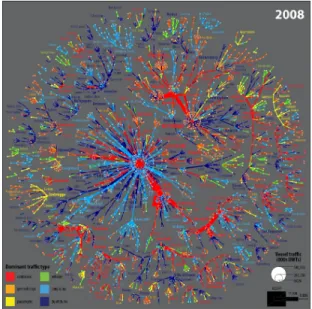
A widespread visual design consists in encoding layer information using node colour or shape, as de-picted in [41, 74, 90, 133]. Colour coding of edges is also used in [30, 35]. This design choice relies on the law of similarity of Gestalt theory (colour similar-ity in this case). This design is often adopted when the multivariate nature of the network is the driv-ing motivation of the visual design. For instance, Figure 6 represents flows of maritime traffic using colour to encode different modes of shipping (or lay-ers). The analyst looks among other things at struc-tural changes over time, where different layers en-code different time slices (Task category D2). But if the analyst is interested in analysing a given time slice, different layers may represent different shipping modes. The related task consists in comparing struc-tural differences among the different modes. In sim-ilar visual designs, layer information is diffuse,

rela-tionships between layers and within the same layer are mixed and users seldom get a handle on layers to manipulate them directly. Nodes belonging to dif-ferent layers are intertwined in the 2D plane, when standard node-link layouts are used, and edge clutter is problematic. Layer-related tasks may therefore be difficult to carry out under these circumstances.

While not explicitly designed with multilayer net-work visualization in mind, constraint based layouts offer the possibility to constrain a two dimensional node-link layout in such a way that respects the con-cept of layers. For example the SetCola constraint-based layout of Hoffswell et al. [59] allows users to ap-ply layout constraints to sets of nodes, which might easily correspond to layers. Such a layout approach supports analysing cross layer connectivity (Task cat-egory A) as well as layer comparison (Task cate-gory D2). The examples covered by the authors in-clude a food web networks and a network modelling a biological cell, and both of these datasets can be considered to have multilayer characteristics.

Figure 6: A multilayer network visualization describ-ing the flow of maritime traffic. Nodes represent ports and different edge colours represent different modes of shipping, taken from [35].

Inspired by the multi-level nature of some

prob-lem areas e.g., biological networks, the 2.5D approach materialises layers as 2D translucent parallel planes in a three dimensional layout, similar in spirit to Fig-ure 2. This visual design relies on the law of uni-form connectedness of Gestalt theory. It separates links lying within layer from those between layers providing a more natural support for path related tasks (Task categories A and B) than traditional 2D node-link layouts, but 3D navigation is required to allow the user to change his perspective on the data and resolve visual occlusion problems. As opposed to 1D axis-based representations, the parallel 2D planes provide space to lay out intra-layer links. In the 2.5D category, some approaches use colour redundantly to encode layer information as in [41]. Other visual de-sign options for 2.5D consist in using colour to en-code an attribute value or a computed metric, e.g., community assignment by a community detection al-gorithm as in [30], across the different layers. From the biological domain, the Arena3D application visu-alizes biological data using an interactive 3D layout, where layers are also projected onto planes, and enti-ties are connected across layers by edges rendered as 3D tubes. The authors demonstrate its effectiveness by analysing the relationship across layers, based on proteins and genes associated with a specific disease (Task category A).

The use of three dimensional layouts is much less common in the information visualization re-search community. While some work has shown that there may be some benefit to three dimensional lay-outs, this is only under stereoscopic viewing tions [126]. Outside of stereoscopic viewing condi-tions, there are no empirical studies which demon-strate usability gains from a three dimensional graph visualization [50].

A more widely accepted approach in information visualization, especially for the purpose of compara-tive analysis of graphs, consists in using small mul-tiple views. This is often used for graph matching tasks, where the focus is on understanding common-alities and differences between a set of related net-works [54]. In the context of this paper, the net-works that need to be matched are distinct layers in a larger multilayer network (Task categories D1 and D2). Whether in a 2.5D setting or in a flat small

multiples setting, one challenge consists in ensuring that duplicate nodes are laid out consistently across layers, by introducing constrained layout strategies as in [41,54] to better support cross layer entity com-parison (Task category B).

More generally, coordinated multiple views are of-ten used in the domain of information visualization, and in many applications e.g., the analysis of mi-croarray data [106]. In this case, two-dimensional node-link views may be used as one of multiple com-plementary visualizations of a multilayer network, e.g., [46, 66, 118]. It is yet possible to eschew the idea of using a node-link visualization altogether [37]. Co-ordination between views is common, e.g., brushing and linking. The Detangler [102] application builds on this by also harmonising layouts between views. It supports several task categories identified in this survey, namely cross layer connectivity (Task cate-gory A), layer manipulation (Task catecate-gory C) and layer comparison (Task categories D1 and D2).

Edge Visualization The complex structure of multilayer graphs makes edge visualization an impor-tant challenge. It may be imporimpor-tant in some cases to distinguish between inter-layer and intra-layer links, in other cases the number of layers may cause enough clutter with respect to edges, that a visualization be-comes less understandable. In some cases, the cho-sen solutions is to simply not draw all edges and to allow the user to choose which edges to see via in-teraction to ease inter-layer comparisons (Task cate-gory B). For example, the PNLB (Parallel Node Link Bands) technique [46] only draws inter-layer edges between nodes on parallel axes, and intra-layer edges are displayed in a separate visualization. The well established technique of edge bundling [60] has been adapted for the multilayer use case by [15]. The au-thors bundle all edges in a single visualization, in an aesthetically pleasing manner, with edges being kept adjacent to each other when they share a common path, and edge crossing being avoided (see Figure 7). This approach is useful for showing edges from mul-tiple layers in a single visualization (where there is no division of nodes between layers); the approach is agnostic to the source or target layer, or whether the

edges are between or within layer(Task categories A and B).

Figure 7: The multilayer edge bundling of [15]

Within their list-based view [28] use edge bundling between different list columns as a clutter reduction techniques clarify similarities between different edge types. The authors essentially group edges based on relation type, by clustering the vertices and altering the clustering based on vertex mode. They also use a modified edge bundling in their circular layout, that distinguishes within-mode edges and between-mode edges, see Figure 8.

4.3.3 Matrix-Based Visualizations

Standard node-link representations of graphs give equal importance to nodes and links and aim usually to convey structural properties of the graph at hand. They may however be difficult to read due to edge clutter for moderate size graphs, and for more com-plex networks encountered in many real usage scenar-ios. When dealing with large and/or dense graphs, matrix-based representations were found to be more

Figure 8: Edge bundling as utilised by [28]. Within category edges are routed around the exterior of the circle. Between category edges are routed via the interior of the circle and bundled.

readable than node-link diagrams [48] for many tasks, except path finding. They consist in laying out nodes as the rows and columns of a 2-way table. A link be-tween two nodes is often represented as a rectangle at the intersection of the associated row and column. This avoids altogether the edge clutter problem of standard node-link representations. Colour is often used to encode the weight of the links, when link at-tribute values are available. This makes matrices very similar, if not identical in essence, to heatmap views frequently used in biology and other domains [129]. Other visual designs include using circles at the in-tersection of rows and columns with size and colour encoding link attribute values, as in [24]. Matrix rep-resentations have been used to visualize homogeneous graphs (nodes of one type), e.g., in software engineer-ing [120], and bipartite (or 2-mode) graphs, e.g., in software performance tuning [47].

The ability to detect link patterns in a matrix view is conditioned by the use of an appropriate order-ing of rows and columns. Various seriation

algo-rithms [23, 39, 84] reorder the rows and columns of the matrix to create dense rectangular blocks of links. Community detection in a bipartite graph consists in finding groups of nodes in one layer which are densely connected to groups of nodes found in the second layer (Task category A). 2-way hierarchical cluster-ing is commonly used with biological data for this purpose. The BicOverlapper system [106] uses bi-clustering methods to find such relationships between groups of genes and related groups of medical condi-tions. On the visual side, BicOverlapper uses coor-dinated multiple views, one of which employs convex hulls within a standard node-link representation to materialise groups of genes, akin to the notion of ele-mentary layers described in Section 4.2. The overlap-ping convex hulls are meant to support the identifica-tion of commonalities and differences between layers (Task categories B and D2).

In presence of multiple layers, the comparison of link patterns between many pairs of layers may be useful to the analyst (Task category A, see Sec-tion 4.1). Laying out small multiples of matrix views side by side is one approach. Liu and Shen [86] in-vestigates several possible juxtaposition strategies, and assess their usability with multifaceted, time-varying networks. MuxViz [30] uses matrices to sum-marise layer-level statistics, as a means to convey a notion of layer similarity to the analyst (Task cate-gories A, B, D1, and D2).

4.3.4 Hybrid Approaches

Recent work has been exploring the integration of multiple visualization techniques, as an effort to bet-ter grasp underlying data [65]. Although matrices have been shown superior to node-link diagrams for dense networks, the latter may facilitate the track-ing of edge directions. In this spirit, NodeTrix [57] mixes node-link views with matrix-based visualiza-tions to support typically locally dense social net-works. While NodeTrix is not explicitly a multilayer network visualization technique, it is the first hybrid approach that focused specifically on network visu-alization. Since its inception, the idea has been ex-tended by other techniques to support other types of data, such as compound graphs [105]. Although they

do not always focus on visualizing multilayer net-works, such approaches could also be directly reused or adapted to support multilayer networks. Vis-Link [25], for instance, allows visualizing a data set using multiple representations at once, also explic-itly displaying the cross-views links. Using the tech-nique, one layer could be used for each representa-tion, and inter-layer links could be highlighted (Task category A). Adopting another perspective, Hybrid-Vis [87] allows using the same kind of representa-tion, but for different levels of details (or hierarchi-cal shierarchi-cales). In this case, a node-link view may in-clude some levels that are shown as expanded, and other levels are shown as collapsed (Task category C). With additional views (histograms, parallel coordi-nates) more details on level attributes can also be obtained (Task categories D1 and D2).

4.4

Interaction Approaches

The discussion about user interactions may be grounded in Yi et al.’s categorisation of interaction techniques [132]. According to Hascoët and Dragice-vic [54], multilayer network visualizations may sup-port user interaction at the level of individual net-work elements (e.g., individual nodes and links), and at the level of whole layers whether single layers or groups of layers (Task category C). They argue that layer level interactions require a visual affordance. In particular their system, called Donatien, supports the Yi et al. reconfigure and explore interactions.

Traditional interactions include:

• selection: point and click selection, lasso selec-tion of nodes;

• filtering: keeping/removing nodes or links based on attribute values;

• navigation: to visually inspect a fragment of the visual representation using zoom and pan, or context+detail techniques (e.g., fisheye distor-tion or magic lenses).

These have obviously been used widely with stan-dard node-link representations, and are directly ap-plicable one layer at a time in the context of mul-tilayer networks. Interacting with entire layers is

however more relevant to the present discussion and ties back to layer level tasks described earlier in Sec-tion 4.1 (Task categories D1 and D2). Donatien offers three different spatial organisations of layers: 1. small multiples; 2. stacking the layers on top of each other; 3. animation. Starting from the small multiples view, the analyst can drag and drop a layer onto another one, to stack them and more eas-ily compare their elements based on the distinctive layer colour. In the stacked mode, a set of title bars provides an affordance to reorder the layers in the stack interactively. The title bars also include re-configuration tools e.g., choices of layout algorithms that are applied to the layer being manipulated or to the whole stack of layers. Crossing-based interaction across the set of title bars is used to achieve flipbook animation, also for the sake of comparison across lay-ers. This seems quite a natural approach when the layers are defined as consecutive snapshots of a dy-namic network. Also in the stacked mode, Donatien clusters nodes from different layers together based on their spatial proximity in the pixel space. The ana-lyst is yet allowed to edit the resulting clusters inter-actively by pulling a node out, or by dragging and dropping a node on another node (or group of nodes) to merge them. Merged nodes carry a colour coded pictogram relating them to the layers they occur in.

More structured layer organisations may prove to be necessary e.g., a hierarchy of layers. This ensues from the concepts of aspects, layers and elementary layers put forth by Kivelä et al, but also to many real application needs. From an interaction perspec-tive, merging layers together or splitting them apart becomes a matter of collapsing or expanding their parent node in that layer hierarchy. In this vicinity, the Ontovis system [112] uses an ontology visualiza-tion to steer the associated network visualizavisualiza-tion. An ontology could be seen as an artifact representing the layer structure of a multilayer network.

The Detangler approach [102] combines two dis-tinct, synchronised visual representations. A first panel (Figure 9, left) displays the overall network con-nectivity through a node-link view between nodes of all layers. Another panel (right) displays a node-link view showing how layers interact (where interaction is measured and inferred in an ad hoc, domain

depen-dent, manner). Detangler supports a “leapfrogging” interaction: the selection of nodes in the left panel au-tomatically triggers the corresponding layers in the right panel (Task category A). Leapfrogging (exe-cuted by double-clicking the selection lasso) expands the original selection to include all nodes (Boolean OR) involved in any one of the layer that got se-lected; or restricts the original selection to nodes in-volved in all layers that got selected from the layer view (Boolean AND).

The OnionGraph application [113] provides a hier-archical focus and context approach targeted specifi-cally toward heterogeneous data. The hierarchy pro-vides different levels of abstraction based on node type, role equivalence and structural equivalence. In their example use case, using an academic publica-tion dataset, the heterogeneity of the data is derived from node types, and edges only exist between certain node types. There is no formal layer definition and the abstraction used to provide the hierarchical fo-cus and context abstraction is applied across all data types and does not fully consider the heterogeneity of the data. Such abstractions could be adapted to be applied on a per layer basis. This could be very use-ful in multilayer systems, particularly for comparison of complex layers.

4.5

Attribute visualization

As with standard network data, node and edge enti-ties in multilayer networks may have many attributes, either categorical of numerical, associated with them. However within a multilayer network, attributes of nodes are not only considered within a single network context. Attributes need to be considered across lay-ers, and attribute values (especially for numerical at-tributes) may change across layers, especially if the attributes are derived from graph metrics, which may be calculated on a per layer basis. An example of this can be seen in the MuxViz toolkit [30]. Here the authors use an annular ring visualization approach, which show the values of metrics across layers, with each ring representing a layer, or in some cases a different centrality for a specific layer see Figure 10 (Task category D1 or D2).

This basic approach involves completely separating

the attribute visualization from the graph structure. To better relate the relationship between networks structure and attributes, the attributes may be inte-grated into the network visualization itself, (referred to as augmented network visualization by [32, 104]) or a linked view brushing approach maybe taken, by which the relevant related nodes would be highlighted in a network view, when selected in the attribute vi-sualization and vice versa (Task category B).

The standard multivariate visualization of paral-lel coordinates is also a suitable basic visualization technique. In the case where the graph is multiplex, and nodes appear in all layers, the different axes can represent a specific layer attribute. Heat maps may also be adapted for a multilayer use case. For exam-ple, the temporal heat-maps of Grottel et al. [51] are made suitable for multilayer attribute visualization, by using graph layers instead of time slices for each column (see Figure 11).

An interesting example of categorical multivariate data in a single layer, which could be extended for multilayer visualization can be seen in the multivari-ate graph analysis tool of Pretorius and van Wijk [97]. Their approach uses icicle plots to describe the (hi-erarchical) categorical attributes of the source and target of a set of directed edges. The source icicle plot is on the left side of the screen and the one for the target nodes is on the right, with the edge and their associated data drawn in the middle. Such an approach may be easily adapted to compare cat-egorical labels across layers Task category B). Com-bined with edge bundling, as done by Holten [61] with Hierarchical Edge Bundling, it could also be used to examine structural and categorical attribute difference between layers simultaneously (Task cate-gories B and D2).

It is also possible to consider categorical attribute data as a network layer in and of itself. For ex-ample, in the application OntoVis [112], Shen et al. use a node ontology graph to query a large hetero-geneous social network dataset. The node ontology graph reflects the disparity of the attribute (how well distributed it is across nodes), and its edges display frequency of links between the entities. It acts both as a visualization of aggregated categorical data, and a layer by which the dataset can be better interacted

Figure 9: A screen shot from Detangler [102] showing how nodes (left panel) relate to layers (right panel). Selecting layers (lasso) trigger the selection of nodes they involve (red nodes, left panel).

Figure 10: A screen shot from MuxViz [30] showing the values for a centrality across layers. Each ring specifies a different layer.

with and understood.

The approach used for attribute visualization relies heavily on the task the user is performing. For exam-ple a scatter-plot matrix is one technique by which attributes may be summarised, possibly even across layers. However if the user’s goal is to understand correlations of attributes across layers, an approach such as the modified multilayer version the scatter-plot staircase (SPLOS) of Viau et al. [124] may be more efficient in terms of comprehension and space.

Figure 11: The Temporal heat Map of [51] showing changes in attribute values over time slices.

In this approach scatter-plots of the attributes are ordered pairwise based on correlation and common axes.

Attribute visualization also can be combined with interaction withing the context of multilayer graph visualization, to help better understand the connec-tion between layers. The Detangler applicaconnec-tion [102] visualizes the level of entanglement of a selected set of nodes by colouring the selection lasso (an attribute measuring internal cohesion of a group – as opposed to group inertia or entropy [110], also proposed in [6]).