Design of a fluidic test bed for MEMS piezoelectric energy harvester

Design of a Fluidic Test Bed for MEMS piezoelectric Energy Harvester

By

Christopher P. Farm

SUBMITTED TO THE DEPARTMENT OF MECHANICAL ENGINEERING IN PARTIAL FULFILLMENT OF.THE REQUIREMENTS FOR

BACHELOR OF SCIENCE IN MECHANICAL ENGINEERING AT THE MASSACHUSETTS INSTITUTE OF TECHNOLOG

JUNE 2006

AUG 0 2 2006 © 2006 Christopher Farm

All rights reserved LIBRARIES

The author hereby grants permission to distribute and reproduce this thesis under the supervision of faculty at Massachusetts Institute of Technology in whole or in part.

Signature of Author...

.

...

Christopher P. Farm 5/13/2006

Certified By ... _...

Sang Gook Kim

Associate Professor o Mechanical Engineering

· _,_____ ~Thesis Supervisor

Accepted By. ... .. ... ... John H. Lienhard V Professor of Mechanical Engineering Chairman, Undergraduate Thesis Committee

Design of a Fluidic Test Bed for MEMS piezoelectric Energy Harvester

By

Christopher P. Farm

Submitted to the Department of Mechanical Engineering On May 16, 2006 in Partial Fulfillment of the Requirements for the Degree of Bachelor of Science in

Mechanical Engineering

Abstract

This document outlines the basic theory behind generating mathematical models, choosing materials and designing geometries for simulating a 900 mile Alaskan Pipeline. The use of dimensional analysis is useful for simulating the vibration spectrum given off in the pipeline due to turbulent flow of the fluid. In the design of PMPG devices, that transform

the mechanical vibration to electrical energy, the scaled down model will be used as a test

bed for future prototype PMPG designs. After modeling the Alaskan pipeline and

designing it around dimensional analysis, a Vernier Low-g accelerometer is used to measure the vibration spectrum. The frequency that was analyzed was 251.01 ± 0.447 Hz

and when converted back to the Alaskan pipeline we achieved a frequency of 6.94Hz.

Using this information we can design PMPG devices that will resonate in this frequency bandwidth to create a higher efficiency in mechanical to electrical conversion.

Thesis Supervisor: Sang Gook Kim

TABLE OF CONTENTS

1. INTRODUCTION AND BACKGROUND ... ...5

1.1 Design of PMPG ... 6

1.2 Other Designs of PMPG Devices ... ... 8

1.3 Alaskan Pipeline System ... 9

2. MODELING THE SYSTEM ... 11

2.1 Natural Frequency Effects ... 11

2.2 Scaled model Equation for Natural Frequency ... 13

2.3 The importance of Reynold's Number ... 15

2.4 Vortex Induced Vibration and the Strouhal Number ... 18

2.5 Internal Induced flow effects on Vibration ... 18

2.6 Modeling Conclusions ... 22

3. SYSTEM DESIGN ... 23

3.1 Meeting Engineering Requirements . ... 23

3.2 System design for Pipeline ... 26

3.3 Pump Vibration Isolation ... 28

4. TEST PROCEDURES ... 30

4.1 Experimental Procedure for Flow Induction ... 30

4.2 Experimental Results for Fluid Transport ... 31

4.3 Figuring out the Alaskan Pipeline's Vibration ... 35

5. CONCLUSION ... 36

LIST OF FIGURES AND TABLES

Figure 1- Cross Section of concept PMPG device... .... 7

Figure 2- Spiral Energy Harvesters ... 8

Figure 3- Pictures of the real pipeline ... 9

Figure 4- Model of the pipe system ... 12

Figure 5- Viscosity dependence on Temperature ... 24

Figure 6- Defining pi groups and Characteristics for Design ... 25

Figure 7- Test Bed Designs ... 27

Figure 8- Pump Model ... 28

Figure 9- Bode Plot Transfer Function for Pump ... 29

Figure 10- Picture of Experimental Setup...31

Figure 11- Logger Pro Software ... 32

Figure 12- FFT Plot ... 34

Table 1- Constituents of the real pipeline ... 10

Table 2- Pi Groups for matching mockup & real Systems ... 21

Table 3- Flow Calculations ... 26

1. INTRODUCTION AND BACKGROUND

One of the biggest concerns society faces in the intense communication and sensing technology age is the finding solutions to pervasive energy sources for the portable devices. Current methods have very limited life times and supplies are depleting rapidly, leaving very little options to maintain the demanded requirements for power at remote locations. In an economic response to supply and demand, people are voicing a higher need for new ways to harvest energy for wireless systems.

Professor Sang Gook Kim and his colleagues at the Massachusetts Institute of Technology have taken on part of an effort to drive for a new type of technology which harvests small mechanical disturbances transforming them into electrical and usable energy.

They have developed energy harvesting techniques using MEMS devices coated with piezoelectric films on nano-scale cantilevered structures. MEMS, otherwise known as micro-electro-mechanical systems, covered with a thin film of piezoelectric material have been known to generate electrical power when stimulated mechanically. The purpose of these MEMS devices will be to generate enough energy to power small wireless sensors at remote locations where wired power or replacing batteries is not possible. They can be applied to national pipelines, aircrafts, ships, computers and a whole range of other devices that require sensors for detection capability and

monitoring around the clock.

Hierold, Christopher. "From micro to nano-systems: mechanical sensors go nano". Zurich, Switzerland: Department of Mechanical and Process Engineering, 2004.

The early technologies of using environmental sources as a means for new age energy have mainly been focused on harvesting the energy through the sun,

geothermal sources, and large dams or rivers. Although constantly being worked on to improve efficiency in these areas, another means of power can be generated by

parasitic disturbances. These vibrations are so small that it's impossible to interact with on the macro level but still exist all around us; it is our intention to retain this unused energy and re-use it for a directed purpose. Parasitic vibrations such as sound in the air, turbulent flow in pipelines, or the rumbling of an engine produce enough mechanical strain in piezoelectric material to realize a possible solution to harvesting this energy. This material uses mechanical strain to convert to electrical charge which indicates a clear possibility for harvesting energy. There have been several designs constructed by Professor Kim's group at MIT to realize the best way of harvesting these outside sources.

1.1 Design of the PMPG

The design of the PMPG is fairly simple. Although there have been many recent changes to its geometry to maximize the performance of the PMPG, the following concept still remains a critical one. In the early stages of development the cross section of the device looks like Figure 1. You can see that this structure resembles the classical design of a cantilever with a mass, also known as a "proof mass" on the end for extra strain and deflection during vibration.

1- - -d

-- +--

-

\

Figure 1. Cross section of concept device in d33 mode of vibration. This can be modeled as a simple cantilever beam2.

Figure 1 shows the orientation of the electrodes in the d33mode whilst there is another orientation of the electrodes, d31, which positions the nodes on the top and on the bottom. In the d33 mode we gain a slight advantage in the output of electrical energy which won't be needed for discussion in this paper3_.

The result of this design is about the size of a dime and needs to be tested in a way that we will be able to tune our device's natural frequency to the frequency of the host which we are collecting energy from. The reason for matching the frequency to our natural frequency is simple. When our devices is operating at its natural frequency it is then deflecting the most at this mode giving us the highest strain and as a result the most power output. There are theories4 _{that relate the amount of output to both the} stress and strain based on the type of deposit and material properties that are given in the design. The following equation shows the relationship that strain, , has with output voltage E.

P

5

PE

2 Choi, W.J. Jeon, Y., Jeong, J-h, Sood, R. and Kim, S.G. "Energy Harvesting MEMS Device based on thin Film Piezoelectric Cantilevers." Cambridge, MA. MIT.

3 Kim, Sang Gook "Energy Harvesting Piezoelectric MEMS Devices for Self-Supportive Wireless Sensors."

In this equation Beta represents the piezoelectric constant that is experimentally determined on the geometry of the design and the type/amount of material that is used. Using this logic we can confirm that maximum deformation of the PMPG will allow us greater output related to the piezoelectric constant, justifying that we need to match our PMPG's natural frequency (where there is maximum strain) to the

frequency of our host.

1.2 Other Designs of PMPG Device

Sometimes to change the natural frequency of the PMPG device, new

geometries need to be exploited. In some recent applications, resonant frequencies of the PMPG devices require low vibration structures, subsequently requiring a longer cantilever for the basic design. However, with these added restrictions on frequency, sometimes this requires that the cantilever model to be made significantly, longer almost so it is infeasible. A few other alternatives have been developed. Serpentine structures shown in Figure 2 are made to resonate in the 150Hz category. These structures are about the size of a fingernail and are made for applications to harvest turbulent flow vibrations in pipe systems.

Figure 2. Spiral energy harvesters designed by Professor Kim's group at MIT5.

5 Choi, W.J. Jeon, Y., Jeong, J-h, Sood, R. and Kim, S.G. "Energy Harvesting MEMS Device based on thin Film Piezoelectric Cantilevers." Cambridge, MA. MIT.

1.3 Alaskan Pipeline System

After understanding the design of the PMPG devices and the types of resonant frequencies that have been achieved, an application for this device needs to be found. The Alaskan pipeline, also known as the Alyeska Pipeline, is an 800 mile pipeline delivering oil in the North American continent to ports in the southern part of Alaska. From these ports the oil is shipped to the rest of the United States for refinement and use.6

Because of the harsh weather conditions in Alaska, the pipeline undergoes constant maintenance by the government. There have been many incidents over its lifetime that indicates a need for sensors of many types to monitor the heath and status of the pipeline: fluidic sensors, temperature sensors, vibration sensors to name a few. It is the intention of this project to develop a PMPG device to power these needed

sensors using the parasitic vibration generated in the pipeline. Figure 3 shows a small picture(s) of the Alaskan Pipeline.

Figure 3. Pictures of the real pipeline.

The first thing that needs to be understood about how to integrate the PMPG to the pipeline is the type of frequency we are looking at on the pipe. Two types of vibration

can be observed: vibration from natural frequency and flow induced vibration. We will discuss how to model these two modes of disturbance in the next section and the roles that they will play in determining the frequency output for the PMPG device to harvest.

Some of the main physical statistics and information for the pipeline and its constituents also follow in the Table 1.

Table 1. Constituents of the real pipeline that need to be modeled.

Density Oil 973 kg/m^3

Diameter Pipe 1.22 m Length Between Studs 18.29 m

Viscosity 2.52E-02 kg/m.s

Kinematic Viscosity 2.59E-05 m^2/s

Thickness 0.095 m

Q (Flow Rate) 3.82 mA3/s

Although we have a rough idea on the range of frequencies that we are looking at when creating the PMPG device, 120Hz-250Hz, a more accurate figure needs to be established in order to create the most efficient power generating MEMS possible and suited for resonance. The idea to design a test bed or a simulation of the real pipeline needs to be scaled down from its original length to simulate at the laboratory. This idea will use the following mathematical models to estimate the frequency of the real system.

2. MODELING THE SYSTEM

To model the pipeline we first recognize that the vibration has three

characteristics inherent in the system natural frequency, turbulence and fluid flow. The next sections will analyze all parts of the design and effectively limit our model to develop the right output.

2.1 Natural Frequency Effects

By using a simple under-damped system revealed in many system dynamic textbooks, we can develop an equation that relates the natural frequency to the mass, the damping ratio (=b/2wn) and the spring constant of a given system. It follows that solving for the displacement over time for the differential equation (2) using the Laplace transform method yields7 equation (3):

mx"+kx=O (2)

x(t) = xO cos -t (3)

m

Here we can see that the natural frequency wn is defined by:

wn =fk/m) (4)

This solution gives an idea to what we might expect in the pipeline that we are constructing at the lab and the pipeline that exists in Alaska. If both structures have the same natural frequency, then it could mean there is a good correlation between the mock-up system and the real Alaskan pipeline. The next step that is necessary to the estimation of the natural frequency is figuring out the variables in Equation (4).

The easiest way to find the natural frequency is to solve for the variables k, the spring constant, and m, the mass, using methods in solid mechanics; this enables us to calculate the natural frequency inherent within the pipeline.

We can see from Figure 3 that a free body diagram can be developed that has a cross sectional design of a pipe with given dimensions in Figure 4. It will have two points that will be supported by uprights from the ground and extend freely across the gap of length L = 60'. The diameter marked here is 48" or 1.22m with a thickness of roughly .095m. These dimensions will help us determine the geometric effects towards

stiffness.

I

A

A

01.22

Figure 4. Model of the pipe system.

With this model, the characteristics for the spring constant is determined assuming a force applied will be in the center of the beam and the bending relationship follows EI = K where K is the curvature relationship, I is the moment of inertia and E is the elastic modulus8. Knowing the effects from geometry (I) and the material (E), the

8 _{Crandall, Stephen & Dahl, Norman & Lardner, Thomas. An Introduction to the Mechanics of Solids.}

USA: McGraw-Hill, 1999. 2

z

beam will deflect under force according to the following series of equations where the modulus of elasticity for steel is 200 GPa.

F = k = 48EI (6)

L3

I-= r (ro4 - ri) (7)

2

Using this relationship we can figure out the spring constant of the system in Equation (8) relevant to our differential solution for the natural frequency. Equation (8) solves for the parameter k in Equation (6) to find the characteristic spring constant in the pipeline.

k = 48EI (8)

L3

Next we will figure in the mass of the system. The mass will simply be the amount of material of pipeline multiplied by its density of steel.

m = pAL (9)

Using these relationships we can then solve for a frequency by plugging in equations (8) and (9) into (4) to obtain the natural frequency. This produces a natural frequency of 122.54 Hz, well within the range that can be matched by the PMPG device and proves that in this model there is some feasibility recognized.

2.2 Scaled Model Equation for Natural Frequency

Now that we've seen the effects of natural frequency on the real pipeline in Alaska, the goal is to scale down this system to a mock-up in order to match this frequency in the lab. In order to do this, we'd like to determine some of the

restrictions that the laboratory model would need to have in order to reach the same type of natural frequency found in the field. In mathematical terms we would like to mimic the following situation:

W model = W real system

Where is the frequency in an un-damped system we have the following restrictions on the model's dynamics:

(k/m) I model = (k/m) real system

Plugging in Equations (8) & (9) again, keeping track of the model constants and real constants, we have the following restrictions set on the diameter, thickness, material properties and length of the model.

ai = ast (Et/Ei)(pi/pst)(Li4/Lst 4 ) (10)

where a= (ro4 - ri4) (11)

(ro2 -ri2)

This is the scaled model equation for natural frequency determination in pipes. The "a" tells the thickness and diameter needed to replicate the real system. The subscript "i" represents the mock-up's characteristics for young's modulus, density and length between posts. The subscript "st" represents the real systems characteristics. We can now use this equation to help us define certain restrictions on our test bed when taking

equation must be satisfied given the parameters of the real pipeline and the parameters of the design.

This Equation also gives insight into the relationship between the pipeline and the mock-up. In equation (10), the ratios that come from the scaled model equation are all proportional except for the diameter, thickness and the length. This relationship is also very useful because it allows us to change different parts of the design and

compensate them in other parts. For example, if the user didn't' want to use steel to construct the mock-up like the pipeline in Alaska, he could use copper and change the geometry so that it would have the same effect on the stiffness of the system.

The significance of this equation gives us restrictions on our design from the standpoint of natural frequency in the model. It is a very robust way of solving for a similarity in the real pipeline and the test bed.

However, natural frequency isn't the only thing that causes disturbance in the pipeline. There is also the turbulence from fluids and vortex induced vibration that can affect the vibration spectrum. Once we can determine how vibration comes from the fluid flow, we can then apply this to our test bed.

2.3 The Importance of Reynolds Number

Reynolds number is probably one of the most remembered dimensionless numbers covered in the study of fluid mechanics. It gives the user a good gauge on the type of flow that goes on within any given closed surface. The three types of flow that this setup is most interested in are turbulent, transitional and laminar. Reynolds number is assigned a critical value at which the flow becomes turbulent, transitional

and laminar. This critical value will be useful to determine what type of flow exists in the Alaskan pipeline, and the things that we can do to match the same turbulence in the test bed.

In this scenario, because we are trying to harvest parasitic vibrations from the flow in the pipe, turbulence will be directly related to the vibration in the pipe. The more turbulent a region is the more we can expect the pipe to vibrate. To make sure that our mock-up best represents the Alaskan pipeline, matching the Reynolds

numbers in the real system and the mock-up is essential for achieving the same type of flow.

Reynold's number comes from the measure of inertial fluid force divided by the viscous fluid force9. If the inertial forces in the fluid are much greater than the viscous forces we inevitably get turbulence in the flow.

Reynold's number can be calculated in the following way:

Re = pvD//

For a pipe's geometry it's proven that the critical value where flow starts to become turbulent is around Re= 23001°. For the Alaskan Pipeline the calculated Re = 154030, showing that the oil in the pipe is clearly turbulent. We can use this Reynolds number in the Alaskan pipeline to match the Reynolds number in the mock-up system that we design. In theory, if the two systems have the similar Reynolds number, then they inevitably have the same type of flow inside the pipe.

9 Cracalho, Ernest and Brisson, John G. "Thermal Fluids Engineering". Massachusetts Institute of Technology. Chapter 9

'O Cracalho, Ernest and Brisson, John G. "Thermal Fluids Engineering". Massachusetts Institute of Technology. Chapter 9

What we can take away from this calculation is that when making the mock-up, our flow needs to be just as turbulent.

2.4 Vortex Induced Vibration and the Strouhal Number

Vortex induced vibration or VIV is a phenomenon that appears in many fluid structures. It is based on the effects that fluids have on oscillating flows. Because this type of phenomenon exists within all types of flows and in many structures, we need to consider the effects that VIVs could have on the Alaskan pipeline and how we can account for these VIVs in the test bed.

The Strouhal number is another dimensionless parameter that will allow us to match similar types of vortex induced vibration in the test bed to the real pipeline. Not only that, it will allow us to solve for the frequency that the real pipeline exhibits once the vibration in the mock-up is determined. Equation (10) shows how the

Strouhal number is calculated.

St = (10)

Vaverage

The frequency of vortex generation is measured with o, the characteristic length of the pipe is measured with L and the average velocity of the flow within the pipe is

measured with Vaverge. The mission to using the Strouhal number is the same as the

Reynolds number. By building the mock-up and measuring the effective frequency we can solve for the Strouhal number of the test bed. However, what we know about dimensionless numbers is that we need to match the test bed's Strouhal number with

the Alaskan pipeline's Strouhal number solving for the frequency in the real pipeline. As you can imagine this would be the last step in our calculations.

2.5 Internal Induced Flow Effects on Vibration

Aside from natural vibrations, turbulent flow and VIV we also consider the vibrations induced from the fluid inside the pipeline at a more detailed level and how it

interacts more integrally with the pipe. The study of turbulent flow and its effects on vibration is not very widespread and techniques used to model this kind of behavior have not been developed. To understand this physical phenomenon we make a scaled down situation from the dimensional analysis perspective. Hopefully this perspective will also tie into other parts of the two previous models.

Dimensional analysis is a method for reducing complex physical situations to the most efficient form. As Bridgman in 1969 explains, "The principal use of

dimensional analysis is to deduce from a study of the dimensions of the variables in any physical system certain limitations on the form of any possible relationship between those variables."" This means that we can develop a group of dimensionless numbers all of which relate to frequency in the physical pipeline and it will hold for all physical sizes of the system. This analysis is what brought about the Reynolds and Strouhal numbers that we have already seen. Scientists have noticed that these dimensionless numbers have a direct correlation to turbulent flow and VIV

respectively. Similarly we can develop dimensionless numbers of our own to relate to

" Sonin, Ain A. "The Physical Basis of Dimensional Analysis." USA: Department of Mechanical Engineering MIT, 1997.

frequency in the pipeline. We will be able to obtain a set of numbers to make limitations on our test bed and "scale" it down from the original system.

Buckingham, another person who studied the relevance of scaling using dimensionless numbers, developed a theorem on how to derive these groups of numbers. He called this the "Buckingham pi theorem". This theorem set a bunch of rules that allowed a person to calculate these pi groups with consistent and accurate determination. The pi groups held true for all ranges of scales and was proven very useful in a number of dimensions/scales. The pi groups are made up of derived dimensionless numbers that all relate to a physical phenomenon much like the Reynolds number to turbulence and the Strouhal number to VIV.

The first step to determining these groups for our situation is answering the question: what independent variables affect the frequency output in the pipeline? Because frequency will be dependent on a number of variables, all the variables that are listed in the function parameter must be independent from one another to be

considered. This means anything that frequency depends on cannot depend on another variable within the set. For this specific case, our group has decided among the

following independent variables. The frequency Fr can be characterized by the function:

Fr = f(D, Q, p, E, t, ) (11)

This shows that frequency will be determined by a part of six variables. The reasons for each will be listed below:

* D- Diameter: Frequency will depend on the diameter of the pipeline because it has a different effect shown in the mechanics of the inertia

*

* p- Fluid Density: Due to the nature of inertial force of the fluid, density will also help measure (along with Q) turbulence of the fluid.

* E- Modulus of Elasticity: The elasticity of the pipeline will determine the type of movements the pipe can make and how forgiving the material is to the pipe flow.

* t- Thickness of Pipe: This is related to the geometry and the diameter. It

determines the strength of vibration.

*· p- Fluid Viscosity: Like density this helps determine the inertial forces found in the fluid.

With this newly written function and independent variables determined, we use Buckingham's method 2to form pi groups for designing the system. According to the theorem, with 7 variables and 3 different dimensions that make up the variables (mass, time and length), there should be 4 independent pi groups that come out of the

theorem. Taken together, these pi groups represent how the frequency phenomenon in the test bed will be matched with the real pipeline.

7l= (Q/wD) (12)

r2= (ED4/pQ2) (13)

7r3= P/t) (14)

r4= (Qp/D/t) (15)

With this, the designer can calculate the dimensionless numbers for the Alaskan pipeline and construct our model off of these restrictions. The idea here will be to calculate values for (13), (14) and (15) and match these numbers with the test bed. Mathematically speaking, each pi group for the real pipeline must match the pi group for the test bed.

7ri Pipeline = ri I Testbed

Looking closely at Equations (12) and (15) we recognize that they are related to Strouhal and Reynolds numbers respectively! This indicates that our intuition on choosing to relate our mock-up's Strouhal and Reynolds numbers were correct.

Because we have all the variables for the pi groups in the Alaskan pipeline, we can calculate these numbers and figure out the dimensions that the test bed must have to satisfy the same pi numbers. Below is a table of the calculated figures. The real system figures need to match the "Mock-up" system figures in order to have an identical output. We can see that with our design we make sure that this happens.

Table 2. Illustrates the real systems pi groups and the matching mock-up systems pi groups in order to get the exact frequency we desire.

Pi groups Calculation Real Mock-up System

w(D,p,Q,w) Q/wD^3 solve for later Measure

r(D,p,Q,E) EDA4/QA2p 19,340,782 19,340,782

Tr(D,p,Q,t) D/t 12.84210526 12.84210526

After we match all the system requirements we can experimentally measure the frequency related to the test bed and solve for the frequency of the real pipeline using (12). Again this is the same method that we use for Strouhal's number. This frequency can then be used to determine how we make our PMPG device and at what frequency we need to make the PMPG resonate.

2.6 Modeling Conclusions

Although there are four different ways to model the system in our design of the test bed, all of them should be considered when making the entire system work. Some people may argue that one model is more accurate for scaling down the pipeline than the other, however the more information that you can conceive from an engineering perspective the better your chances are for matching the entire real system. In this

case, the engineering from the first model in natural frequency may only contribute roughly 10% of the vibration to the structure, but by including it with the dimensional

analysis, Reynold's Number, and the Strouhal number the mock-up only becomes more accurate.

3. SYSTEM DESIGN

The system design will be composed of two major components, figuring out the dimensions based on section two's equations and also physical system integration. Both are important because they express two extremely important things when

designing any mechanical system: engineering limitation and creativity. In this section we will explore the best options for meeting both criteria. First because it's relatively difficult to find an infinite amount of diameters for pipes that we can use to model the Alaskan pipeline, we need to restrict the size of the diameter to the types of pipes that we can get. Some of the most common diameter sized pipes are .5", 1" and 1.5". Therefore we will start by calculating the pi groups using these diameters calculate the rest of the parameters for the design.

3.1 Meeting Engineering Requirements

In theory we can solve for the type of flow rate or pump we are needed to have given the diameter of the pipe selected. Each of the pi groups, namely Equations (13) and (14) yield a certain flow rate for a given diameter. Because all pi groups in the original pipeline must match the pi groups in the scaled pipeline we have to solve for the flow rate, Q, in Equation (13) and Equation (14); this will allow us to solve for the diameter as well. With two equations and two unknowns, we will be able to solve for them. The flow rate is important in our design to understand what size pump to buy and the diameter to determine what size pipe to buy. We also need to decide that the

fluid that will be pumping be restricted to water as a design requirement in our test

bed.

Because water will be used as the fluid understanding the effects temperature has on viscosity is very important. A brief illustration is shown in figure 5.

Viscosity of water y = 3E-08x4- 9E-06x3+ 0.001x2- 0.0552x + 1.7782 2 1.8 1.6 1.4 1

1.2

Poly. (Viscosity of water)

0 20 40 60 80 . 100 120

Temperature

Figure 5. Illustration on how the viscosity of water changes with temperature3.

In our scenario it works best to choose the viscosity of water at room temperature of 25°C so that a heater doesn't need to be purchased. This makes the viscosity constant set at an approximate kinematic viscosity of approximately 8.90e-7.

Using water and the equations 10.2 and 10.4 we find that D= 1.67" in theory

and will equate the flow rates for all pi groups with copper material. However, because

we are unable to make a 1.67" diameter tube, we will use the 1.5" diameter. In this

situation Microsoft Excel outputs the results for the design in Figure 6.

13 White, Frank M. Fluid Mechanics: Fifth Edition. USA: McGraw-Hill, 2003.

Pi groups I OUTPUT

rr(D,p,Q,w) n/a n/a Gph

w(D,p,Q,E) Flow rate l - 3495.50379

Tr(D,p,Q,t) thickness 0.002966803 0.11680328

Tr(D,p,Q,) Flow rate 0.004100081 3899.22643 Figure 6. Defining the pi groups and meeting the characteristics for design.

We can see here that the flow rate output is roughly 3500 gph when D-= 1.5" in

Equation (13), and 3900 gph when D= 1.5" in Equation (15). This is the closest that we can get to matching the scaled pi groups. Through the ability to change our flow rate, we can measure the different change in frequency through a range of flow rates in our experiment and correctly match the frequency to the first pi group.

Once we obtain the number for "pi group one" we will be able to use this number to back out the real frequency of the Alaskan pipeline. This will let us figure in the natural frequency of the PMPG that is in the design process.

We can also use Equation (14) to find a thickness that is necessary for the scaled model system as well. The excel spreadsheet outputs a size of roughly .12" in thickness. The next design requirement we can look at is the turbulent flow requirement. Since the oil in the pipeline has a turbulent flow, we want to design our test bed to be the same turbulent flow with water. Using the dimensions and the given quantities for Reynolds number, we back out a flow rate shown in Table 3. We can see that we obtain the same flow rate as shown for the Equation (15). This is a very good sign that shows us one of the pi groups that was backed out using dimensional analysis is similar to our measure of turbulent flow using Reynold's number. Our independent variables

in the function are consistent with what we are trying to look at as a whole proving that our assumption of variables is in the right direction.

Table 3. Flow rate calculations are met.

Density Water 1000

Diameter Pipe 0.0381

Ave Velocity

Viscosity 8.90E-04

Kinematic Viscosity 8.90E-07

Q 4.10E-03

Re 154030.9

Volumetric Flow Rate 0.0041

Volumetric Flow Rate

(gal/hr) e

Now that we have a good concept on our target diameter, thickness and our flow rate, we can use these in our "scaled model equation" to determine the length of the pipe between studs. Plugging all variables into Equation (10) and (11) we can solve for a length of roughly 2 meters.

Now that all the design characteristics are set in motion, the pump needs to be designed for at least 4000gph and monitored by a flow meter to be able to change the flow rate when needed. The test bed pipe will be made from copper with dimensions

1.5" OD and .12" in thickness. The change in flow rate will allow us to measure how it correlates to frequency.

3.2 System Design for Pipeline

Now that all the design requirements have been met, the test bed design and schematic needs to be decided. In our schematic we need to make sure that we have

something that will measure the output frequency, absorb any residual vibration from the water pump, measure the flow rate of the water, something that can control the flow rate (variable switch), and a reservoir to store extra water. Outlined below will be a schematic to follow when constructing the test bed.

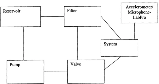
All the water will start and end with the reservoir. This allows for a circular path where the water flowing through the pipe is recycled and more efficient. The reservoir will connect to a pump of specified 4000 gph that will pump into the designed system, gauged by a manual control valve. This will flow into a meter for flow rate measurement and documentation and finally the test bed system. Frequency will be measured via an accelerometer. After through the test bed the water will return back to the reservoir. The schematic is shown in Figure 7.

I . . I

Reservoir Filter Accelerometer/

Microphone-LabPro

System

_ _/

Figure 7. This figure diagrams the entire test bed that we will implement.

Pump Valve

. ~ ~ .

. I~~~~~~~~~~~~ I

The lines connecting each unit will be made out of PVC piping material, and the system made out of copper tubing. Once we can get the measurement of frequency taken care of the flow rate can be varied to see how that affects the output.

3.3 Pump Vibration Isolation

The pump that will be applied in this situation is a Flotec FP5172-08 and meets the requirements of the fluid flow for this test bed. However, because the pump vibrates, it may affect test bed by producing noises. These vibrations could be costly for the PMPG device as we may get a false understanding of the pipe's actual vibration. Therefore, by designing an isolation system for the pump, we can get rid of the

vibrations that could possibly couple with the test bed. We also need to consider an isolation system for flow fluctuations.

In this section we have modeled the pump as shown in Figure 8.

Mass

k b

Figure 8. This figure shows the model of the pump with Mass (m), spring constant (k) and damping constant (b). The input for this will be F(t) = A sin(wt + B)

After setting up the differential equation and taking the Laplace transform with an input of the form A sin(wt + B) we can obtain the transfer function in equation 16.

1

X(s) = 2 (16)

Plugging the numbers for each as A= .001m, w= 60Hz, m= 10kg, b= 50kg/s (blue), 1000kg/s (green) and k= 5N/m we can obtain a bode plot that looks like Figure 9.

Bode Diagram

By using this design with the parameters suggested above, we can see our output will deteriorate by 750% because of the differences in amplitude between both bode plots. With input amplitude on the order of lmm we can expect our amplitude this design will yield an output on the order of micrometers which will not affect the output of our test bed if it is far enough away from our design. To make this setup reality we can construct a wooden table with rubber feet. The rubber will be used to simulate the damping mechanism and the wood will simulate the spring. This will mimic the desired effects explained above and isolate our pump from the rest of the system.

4. TEST PROCEDURES

After the test bed has been built and the pump isolated, we took measurements for the vibration of the pipe while matching the pi groups for the Alaskan Pipeline. We can use instruments such as the accelerometer to measure the vibration and frequency output. You could also use a microphone to measure the frequency with Lab Pro. Since the measurement recorded should lie within the sound spectrum using the microphone should be enough. We will then transform these waves into the frequency domain and analyze where the highest resonance lies. Using the fast-fourier transform analysis (FFT) we can isolate the peaks that the pipe resonates at under the turbulent flow conditions described.

4.1 Experimental Procedure for Flow Induction

After piecing the modules of the system together, including the pipe, the pump, the 3-way valve and the reservoir, we can run water through the pump at

Figure 10. These three pictures are of the setup used for measuring the vibration frequency. The pipeline on the left is isolated from the rest of the pump system so there are no compounding effects. The pump in the middle is also isolated from the rest of the system so there are no compounding effects. The 3-way

valve on the right makes sure that we can control flow and drainage.

The reservoir not shown here simply is a place where the water is recycled from input and output. The main point is to isolate each parts of the system so that there are no discrepancies and compounding effects from each other.

Logger Pro was the software used and a Low-g accelerometer attached to the mid section of the pipeline picked of the frequencies that were needed. The Low-g accelerometer is made by Vernier Software and Technology and its order code is LGA-BTA. The accelerometer uses an integrated circuit (IC) and micro-machined cantilevers in a silcon wafer to pick up the vibrations. In Figure 12 you can see the setup used connecting the accelerometer to the system.

Figure 11. These figures show the Logger Pro software and data collection material. The accelerometer is shown next to the computer. The accelerometer was then taped securely to the copper tubing and

system for data collection.

4.2 Experimental Results for Fluid Transport

The experimental results show that we have an average resonance frequency of approximately 251.01 Hz with a standard deviation of .61 Hz by fitting sinusoid curves to the data. The data actually follows a noisy sinusoid condition and fitting a curve to the data gives us the approximation for the frequency. This means that the 95% confidence interval is very narrow, encapsulating the region of 251.01 ± 0.447 Hz. The data can be seen in table 2. The data shows that the amplitude and phase are relatively inconsistent with the flow, unlike the frequency and the constant. All the vibrations were fitted with the curve "A*sin(wt + phase) + constant". The inconsistency in the amplitude and phase could partially be attributed to the noise that is found in the environment such as sound noise and air currents. These things may have an effect on the amplitude and phase of the pipeline and will be present in the real pipeline. Although these results could possibly show that acquisition of data was inaccurate, we predict that environmental factors will not change the fundamental frequency and the constant that is apparent in the system.

The reasons for this are two fold: (1) the main driver in the vibration is the fluid flow and (2) noisier exist in the real world. To explain these further, the fluid flow will consistently drive the pipeline's vibration rather than be affected by the smaller and less relevant externalities that will exist.

Table 4. This is a summary of the results found from experimentation and curve fitting to Asin(wt + B)+ C, where A is amplitude, w is frequency, B is phase and C is the constant.

Trial Freq (Hz) Amplitude Phase Constant

1 252.00 0.01546 -1.988 -11.74 2 250.80 0.1355 0.9932 -11.75 3 250.00 0.04366 1.15 -11.76 4 250.30 0.1528 3.004 -12.04 5 251.30 -2.566 0.06957 -12.04 6 251.30 7.127 -0.05384 -12.02 7 251.30 -2.555 0.1349 -12.05 8 251.30 -21.49 0.02512 -12.04 9 250.80 0.07848 0.6674 -12.05 'V.^;V ." = 's ' :='.=a: e... ~

The main takeaway, regardless of the other variables, is the frequency. With the designed system and isolation developed from the bellows and dampers, a figure of approximately 250 Hz was obtained. This figure is on the high end of the spectrum that was expected in the introduction (120 Hz - 250 Hz). This means that on the Alaskan pipeline the mock-up system predicts vibrations on the higher end of the spectrum and the PMPG device should be designed appropriately.

Another method, other than curve fitting, to find the unique frequency peaks is the FFT. However, when using this method we find that there are no real distinct peaks that can separate one frequency from the next. An example of a single FFT on a sample run is provided in Figure 12.

i 0.010-Z * a . 4 -0

_.Ron

Figure 12. FFT plot shows inconsistencies with the more rational curve fitting technique in Hz. This most likely incorporates the noisy frequencies that are caused by the external environment and

doesn't clearly reflect the pipelines vibration from induced fluid flow.

As you can see in Figure 12, no real peaks are apparent and the one peak that shoots up around 10 Hz doesn't make any sense with the fitted curve. What could be happening is that our Nyquist frequency is set too low because of our sampling rate of the device. Due to the nature of our measurement tools, we are apparently aliasing the actual frequency of the system and not looking at the real spectrum.

Another problem with the FFT is that we are picking up a lot of noise that can't be filtered out. Because the FFT doesn't exude any apparent resonance, noise attributed from the environment makes it harder to pinpoint what the actual frequency of the test bed is.

For these reasons, the FFT makes it more difficult to consider the frequency of the test bed and the curve fitting method is more accurate for description of the

system. ... .. ... .. ... ... ... ... ... .. ... ... ... ... .. ... .. . I.. . .. .. ... . .. ... ... .... .... ... .. . i I i i I i ---`

4.3 Figuring out the Alaskan Pipeline's Vibration

Now that we have determined the test bed vibration spectrum we can solve for the frequency inherent in the real pipeline using equation (12) or Strouhal's number. Because these two dimensionless parameters are one in the same it doesn't matter which one is chosen.

Knowing that we have a frequency of 251Hz for the mock-up system and all the variables for equation (12) we solve for the first pi group. The number comes out to be in the form shown in equation (17).

test-bed =.30298 (17)

)'test-bed - D3

Theoretically, this pi group should span across all dimensions and equating this to the pi group of the real system we solve for a frequency of 6.94 Hz for the real system. This can be shown in Equation (18).

Qreai = 6.94Hz (18)

test-bed

If you were to use the Strouhal number in place of equation (12) you would find the same result. Here the o is the vortex generation frequency.

5. CONCLUSION

The results of the mock-up were successful. We achieved a value for frequency with 251.01 Hz ± 0.447 for a 95% confidence interval in the test bed. This means the results for the designed test bed are repeatable and efficient in giving an output that was predicted by the modeling. In this case breaking the model down from the

dimensional analysis, mechanics, dynamics and material properties all proved useful in constructing a design with the desired output. After calculating the pi group for the test bed and solving for the real system's frequency we get 6.94 ±0.447 Hz.

Snm rerionc !ave lrtocl rrptlr horn rl,~r.t , .Scr h ,l cnr% r r -A

l-VVIII --osE>^-o *s^Yk wLsk^} VXWL- -11x Wsk*6Ws 31.- -at , . llQALA

mechanical cantilevers, but due to low frequencies found in the real E designs will need consideration to maximize the efficiency of energy

5.1 Future Considerations

Now that we were able to determine the suggested frequency

,nAl eL. , r..l ;,lln- th- rrr....'e n.-. m*,;ir .r.l.l IA -l to l... 1-,

V a.n. 3 a II..lU LAk

ipeline, new ,eneration.

f the test bed - - -- *- At-Lt

,llLU L11 I 1 11.llJI. LIILC 1; LUU 3 IIA1L LIILIIVC W/UlULI L LU V CV4U4LC; 11JW LLUldCL L1113

number of 6.94Hz could be and to also figure out a way to fabricate nd test the PMPG prototypes at this frequency.

To verify the vibration of 6.94Hz, it's possible to go to Alaska and measure the frequency along several points of the Alaskan system. It's very likely that the

frequency of the real system could change over distances and through different terrain. The model that we have created for the test bed does not take into account the levels of terrain, the temperature of the terrain and any external conditions that could affect

the vibrations. The models used to create the frequency in the test bed are dominated by the fluid characteristics and none of the other external factors were considered. The only other way to get a real sense of the vibration spectrum is to measure the actual vibration of the pipeline using an accelerometer in Alaska.

To test upcoming prototypes of the PMPG it's possible to create a new structure that is no longer related to fluids but may be able to vibrate at different frequencies and amplitudes. To simply design a mechanical resonator where you could change the frequency of vibration by sampling turning a knob would make the process of fabricating PMPG prototypes more efficient and effective. It's no longer necessary to use the test bed because our only purpose was determining the frequency in the real pipeline. Since we have already determined this frequency, it's possible to explore other methods of creating the frequencies needed to fabricate new PMPGs.