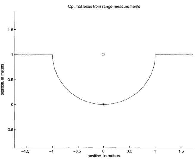
Delayed stochastic mapping

commercial croissant couvert par une entrée de capitaux en provenance du reste du monde.. Baisse de la part des salaires.. Salaires et consommation.. Consommation et

• Mais plus la dette extérieure des Etats- Unis augmente, plus l’arrêt de la. détention de dollars par le Reste du Monde ferait chuter le dollar, et plus il est improbable donc

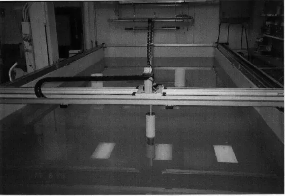
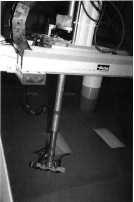
We assessed (i) the acceptability and feasibility of the devises, software, and setup in a clinical setting using a qualitative approach with an observer listing all significant

Trial emulation to explore residual confounding Trial simulation Effectiveness level 1Systematic review of randomized controlled trialsDescription:Identify and aggregate available

Type ‘‘ my first program ’’ (get into the habit of giving descriptive names to projects and other files) in the Target name box. Use the browse button to find the

However, asking physicians and health care professionals whether they consider themselves good communicators is like asking licensed drivers if they consider themselves

Interested read- ers can simply browse the book and choose a topic of interest; reading an appropriate section might be suffi- cient to get some working strategies.. The book

At the individual level, the perceived quality of life of the citizens required to switch from private motorized modes to public transport, intermediate modes, walking and/or cycling