HAL Id: inserm-00629187
https://www.hal.inserm.fr/inserm-00629187
Submitted on 5 Oct 2011HAL is a multi-disciplinary open access archive for the deposit and dissemination of sci-entific research documents, whether they are pub-lished or not. The documents may come from teaching and research institutions in France or abroad, or from public or private research centers.
L’archive ouverte pluridisciplinaire HAL, est destinée au dépôt et à la diffusion de documents scientifiques de niveau recherche, publiés ou non, émanant des établissements d’enseignement et de recherche français ou étrangers, des laboratoires publics ou privés.
Simon Eskildsen, Pierrick Coupé, Vladimir Fonov, José Manjón, Kelvin
Leung, Nicolas Guizard, Shafik Wassef, Lasse Riis Ostergaard, D Louis Collins
To cite this version:
Simon Eskildsen, Pierrick Coupé, Vladimir Fonov, José Manjón, Kelvin Leung, et al.. BEaST: brain extraction based on nonlocal segmentation technique.. NeuroImage, Elsevier, 2012, 59 (3), pp.2362-73. �10.1016/j.neuroimage.2011.09.012�. �inserm-00629187�
Guizard, Shafik N. Wassef , Lasse Riis Østergaard, D. Louis Collins and the Alzheimer’s Disease Neuroimaging Initiative**
a
McConnell Brain Imaging Centre, Montreal Neurological Institute, McGill University, 3801 University Street, Montreal, Canada
bDepartment of Health Science and Technology, Aalborg University, Fredrik Bajers Vej 7D, Aalborg, Denmark c
Instituto de Aplicaciones de las Tecnologías de la Información y de las Comunicaciones Avanzadas (ITACA), Universidad Politécnica de Valencia, Camino de Vera s/n, 46022 Valencia, Spain
dDementia Research Centre (DRC), UCL Institute of Neurology, Queens Square, London, WC1N 3BG, UK
Abstract – Brain extraction is an important step in the analysis of brain images. The variability in
brain morphology and the difference in intensity characteristics due to imaging sequences make the development of a general purpose brain extraction algorithm challenging. To address this issue, we propose a new robust method (BEaST) dedicated to produce consistent and accurate brain extraction. This method is based on nonlocal segmentation embedded in a multi-resolution framework. A library of 80 priors is semi-automatically constructed from the NIH-sponsored MRI study of normal brain development, the International Consortium for Brain Mapping, and the Alzheimer’s Disease Neuroimaging Initiative databases.
In testing, a mean Dice similarity coefficient of 0.9834±0.0053 was obtained when performing leave-one-out cross validation selecting only 20 priors from the library. Validation using the online Segmentation Validation Engine resulted in a top ranking position with a mean Dice coefficient of 0.9781±0.0047. Robustness of BEaST is demonstrated on all baseline ADNI data, resulting in a very low failure rate. The segmentation accuracy of the method is better than two widely used publicly available methods and recent state-of-the-art hybrid approaches. BEaST provides results comparable to a recent label fusion approach, while being 40 times faster and requiring a much smaller library of priors.
Keywords: Brain extraction, skull stripping, patch-based segmentation, multi-resolution, MRI, BET
** Data used in the preparation of this article were obtained from the Alzheimer's Disease Neuroimaging Initiative (ADNI) database (www.loni.ucla.edu/ADNI). As such, the investigators within the ADNI contributed to the design and implementation of ADNI and/or provided data but did not participate in analysis or writing of this report. Complete listing of ADNI investigators is available at http://adni.loni.ucla.edu/wp-content/uploads/how_to_apply/ADNI_Authorship_List.pdf).
1. Introduction
Brain extraction (or skull stripping) is an important step in many neuroimaging analyses, such as registration, tissue classification, and segmentation. While methods such as the estimation of intensity normalization fields and registration do not require perfect brain masks, other methods such as measuring cortical thickness rely on very accurate brain extraction to work properly. For instance, failure to remove the dura may lead to an overestimation of cortical thickness (van der Kouwe et al., 2008), while removing part of the brain would lead to an underestimation. In cases of incorrect brain extraction, subjects may be excluded from further processing, a potentially expensive consequence for many studies. The solution of manually correcting the brain masks is a labour intensive and time-consuming task that is highly sensitive to inter- and intra-rater variability (Warfield et al., 2004).
An accurate brain extraction method should exclude all tissues external to the brain, such as skull, dura, and eyes, without removing any part of the brain. The number of methods proposed to address the brain segmentation problem reflects the importance of accurate and robust brain extraction. During the last 15 years, more than 20 brain extraction methods have been proposed using a variety of techniques, such as morphological operations (Goldszal et al., 1998; Lemieux et al., 1999; Mikheev et al., 2008; Park and Lee, 2009; Sandor and Leahy, 1997; Ward, 1999), atlas matching (Ashburner and Friston, 2000; Kapur et al., 1996), deformable surfaces (Dale et al., 1999; Smith, 2002), level sets (Baillard et al., 2001; Zhuang et al., 2006), histogram analysis (Shan et al., 2002), watershed (Hahn and Peitgen, 2000), graph cuts (Sadananthan et al., 2010), label fusion (Leung et al., 2011), and hybrid techniques (Carass et al., 2011; Iglesias et al., 2011; Rehm et al., 2004; Rex et al., 2004; Segonne et al., 2004; Shattuck et al., 2001). Studies evaluating these methods have found varying accuracy (Boesen et al., 2004; Fennema-Notestine et al., 2006; Hartley et al., 2006; Lee et al., 2003; Park and Lee, 2009; Shattuck et al., 2009). While some methods are better at removing non-brain tissue, at the cost of removing brain tissue, others are better at including all brain tissue, at the cost of including non-brain tissue (Fennema-Notestine et al., 2006; Shattuck et al., 2009). This is a classic example of the trade-off between sensitivity and specificity.
Beyond the technical issues, the brain extraction problem is further complicated by the fact that no accepted standard exists for what to include in brain segmentation. While there is consensus among methods that obvious non-brain structures, such as skull, dura, and eyes should be removed as part of the brain extraction process, there are divergent opinions on other structures and tissues, such as the amount of extra-cerebral cerebro-spinal fluid (CSF), blood vessels, and nerves. Some methods define the target segmentation as white matter (WM) and gray matter (GM) only (Leung et al., 2011), while others include CSF, veins, and the optic chiasms (Carass et al., 2011; Smith, 2002). Depending on the objective for the subsequent analysis it is important to remove tissues that may be confused with brain tissue in the images.
Most brain extraction methods are developed to work on T1-weighted (T1w) magnetic resonance images (MRI), since this is a common modality in structural neuroimaging as it provides excellent contrast for the different brain tissues. In addition, the brain segmentation performed using T1w images can be mapped to other modalities if needed. However, due to the various acquisition sequences and scanner types, the appearance of the brain in T1w images may vary significantly between scans, which complicates the task of developing a brain extraction method that works across sequences and scanners. A further complication is the anatomical variability of the brain. Neuroimaging studies are performed on individuals at all ages with and without tissue altered by pathologies. Therefore, existing brain extraction methods often need to be adapted specifically for a certain type of study or, in the best case, need to be tuned to work on a certain population. A method that works reliably and robustly on a variety of different brain morphologies and acquisition sequences without requiring adjustment of parameters would greatly reduce the need for manual intervention and exclusion of subjects in neuroimaging studies.
Building on recent work on label fusion (Aljabar et al., 2007; Collins and Pruessner, 2010; Heckemann et al., 2006), the multi-atlas propagation and segmentation (MAPS) method (Leung et al., 2010) was adapted to brain extraction to address the problem of variability in anatomy and acquisition, producing more robust results and leading to the best currently published results (Leung et al., 2011). In label fusion approaches, multiple atlases are selected from a library of
previously labelled images. After non-rigid registrations of these atlases to the target image, their labels are merged through a label fusion procedure (e.g.; majority vote, STAPLE, etc.) (Sabuncu et al., 2009; Warfield et al., 2004) to obtain the final segmentation. This type of method is dependent on the accuracy of the non-rigid registrations. Registration errors may result in segmentation errors, as all selected labels are typically weighted equally. Like many of the label-fusion methods, by using a large library of labelled images (priors), MAPS compensates for possible registration errors, which leads to superior results compared to other popular brain extraction methods. However, due to the large library and the time consuming multiple non-rigid registrations step in MAPS, the processing time per subject on an Intel Xeon CPU (X5472 3GHz) is 19 h. Furthermore, in many studies it is not feasible to build a large library of priors and the long processing time may be a bottleneck in the analysis pipeline.
A recent framework inspired by nonlocal means MRI denoising (Buades et al., 2005; Coupe et al., 2008; Manjon et al., 2008) has been introduced to achieve the label fusion segmentation task. This method has demonstrated promising segmentation results without the need for non-rigid registrations (Coupé et al., 2011). Instead of performing the fusion of nonlinearly deformed atlas structures, this method achieves the labelling of each voxel individually by comparing its surrounding neighbourhood with patches in training subjects in which the label of the central voxel is known. In this paper, we present the adaptation of this patch-based segmentation approach to perform brain extraction. The patch-based segmentation method cannot be directly applied to brain extraction, because i) false positives are likely to occur as extra-cerebral tissue may resemble brain within the patch structure, and ii) the computational complexity is high and this becomes a significant problem for large structures. To address these issues, we propose to apply the patch-based segmentation within a multi-resolution approach to extract the brain. We validate the performance of the proposed method on multiple collections of T1w MRI and demonstrate that the method robustly and consistently extracts the brain from subjects at all ages (from children to elderly) and from healthy subjects as well as patients with Alzheimer’s Disease (AD). The main contribution of this paper is the development of a robust procedure to identify accurate brain masks with an extensive validation on multiple datasets acquired on different scanners and from different populations.
2. Definition of brain mask
As mentioned in the introduction, no standard exists defining what should be included and excluded when performing the brain extraction. In our study, we aim to exclude all extra-cerebral tissues, which resemble GM or WM by image intensity and may affect subsequent analyses. Such tissues include the superior sagittal sinus (may resemble GM) and the optic chiasms (may resemble WM). Following this principle, we accept inclusion of internal CSF and CSF proximate to the brain, as the T1w MR signal from CSF is easily separated from non-liquid structures and subsequent analyses may benefit from the inclusion of CSF as noted in (Carass et al., 2011). We propose the following definition of a mask separating the brain from non-brain tissue:
Included in the mask
All cerebral and cerebellar white matter
All cerebral and cerebellar gray matter
CSF in ventricles (lateral, 3rd and 4th) and the cerebellar cistern
CSF in deep sulci and along the surface of the brain and brain stem
The brainstem (pons, medulla) Excluded from the mask
Skull, skin, muscles, fat, eyes, dura mater, bone and bone marrow
Exterior blood vessels – specifically the carotid arteries, the superior sagittal sinus and the transverse sinus
Exterior nerves – specifically the optic chiasms
3. Proposed brain extraction method
The proposed Brain Extraction based on nonlocal Segmentation Technique (BEaST), is inspired by the patch-based segmentation first published in Coupé et al. (2010) and extended in Coupé et al. (2011). As done in Coupé et al. (2011), we use sum of squared differences (SSD) as the metric for estimation of distance between patches. Using SSD as the similarity metric requires that the intensity of brain tissue is consistent across subjects and imaging sequences. Therefore,
we perform intensity normalization and spatial normalization before constructing the library of priors. Because manual brain segmentation from scratch is an extremely time consuming process, and because some automated techniques yield reasonable results, the gold standard of library priors is constructed using a semi-automatic method that involves extensive manual correction of automatically generated brain masks.
The following describes the normalization, the construction of the library containing the priors, and the fundamental patch-based segmentation method as well as our contribution of embedding the method in a multi-resolution approach to improve segmentation accuracy and computation time.
3.1 Normalization
Image intensity normalization of the T1w MRI data is performed by first applying the bias field correction algorithm N3 (Sled et al., 1998) followed by the intensity normalization proposed in Nyul and Udupa (2000). Spatial normalization is achieved by 9 degrees of freedom linear registration (Collins et al., 1994) to the publicly available ICBM152 average (Fonov et al., 2011) that defines the MNI Talairach-like stereotaxic space, and resampled on a 193×229×193 voxel grid with isotropic 1 mm spacing. A final intensity normalization is performed in stereotaxic space by linearly scaling the intensities to the range [0;100] using 0.1%–99.9% of the voxels in the intensity histogram within an approximate stereotaxic brain mask.
3.2 Construction of library
3.2.1 Datasets used
The library of segmentation priors is built from several datasets: the NIH-funded MRI study of normal brain development (termed here the NIH Paediatric Database, or NIHPD) (Evans, 2006) (age: 5–18y), the International Consortium for Brain Mapping (ICBM) database (Mazziotta et al., 1995) (age: 18–43y), and the Alzheimer’s Disease Neuroimaging Initiative (ADNI) database (Mueller et al., 2005) (age: 55–91y). The NIHPD and ICBM databases consist of healthy subjects, while the ADNI database, in addition to cognitive normal (CN) subjects, contains scans of subjects with AD and mild cognitive impairment (MCI). This way, almost the entire human
life span is covered and subjects with atrophic anatomy are included, which provides a representative library of priors for performing brain extraction.
We chose 10 random T1-weighted (T1w) magnetic resonance (MR) scans from each of the NIHPD and ICBM databases. From the ADNI database we chose 20 random T1w MR scans at the time of screening from each class (CN, MCI, AD). In total, our library consists of 80 template MRI images with their associated brain masks described below. All scans were acquired using 1.5T field strength.
3.2.2 Priors construction
Ideally, one would use MRI data with manually segmented brain masks from multiple experts to create the priors. Unfortunately, manual segmentation is heavily time consuming - taking between 6 and 8 h per brain for a 1mm3 isotropic volume to generate a mask that is consistent in 3D in coronal, sagittal and transverse views. Furthermore, inter- and intra-rater variability can lead to errors in the priors. We have decided to take a more pragmatic approach where automated tools are used to get a good estimate of the cortical surface and manual correction is used afterwards to correct any errors. This way, we benefit from the high reproducibility of the automated technique as well as the anatomical expertise of the manual raters. Priors were generated using one of two strategies, depending on the source of the data.
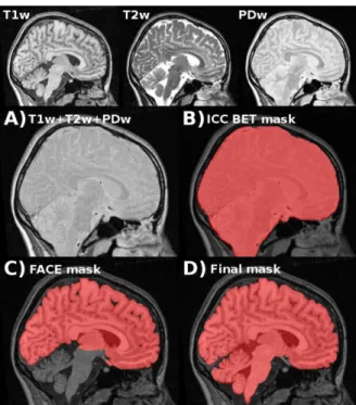
NIHPD and ICBM: The NIHPD and ICBM databases contain T2w and PDw images in addition
to T1w images. T1w images have high signal for the brain tissue, while T2w and PDw images have high signal for CSF (see Fig. 1). We take advantage of this fact to build the priors library. By adding intensities from the three different sequences, we obtained an image with a very high signal for the intracranial cavity (ICC) (Fig. 1A), which could be easily extracted using the widely used Brain Extraction Tool (BET) (Smith, 2002) from the FMRIB Software Library (FSL, http://www.fmrib.ox.ac.uk/fsl) (Smith et al., 2004) (Fig. 1B). From the ICC segmentation, we used Fast Accurate Cortex Extraction (FACE) (Eskildsen and Ostergaard, 2006) to delineate the boundary between GM and CSF in the cerebrum (Fig. 1C). Cerebellum and brain stem were added by non-linearly fitting masks in stereotaxic space. Finally, extensive and careful manual corrections were performed to get an optimal brain segmentation matching our definition (see Section 2) (Fig. 1D). On average, such corrections took between 1 and 2 h per brain.
ADNI: Priors from the ADNI database were constructed using the semi-automatic segmentations
used in MAPS (Leung et al., 2011). These segmentations are accurate definitions of the GM and WM of the brain, but all interior CSF is excluded (see Fig 2A). Therefore, we deformed a spherical mesh initialized around the brain to fit smoothly along the border of the segmentation. In this manner, we obtained a similar definition of brain segmentation as for the NIHPD and ICBM data. Finally, these segmentations were manually corrected in the same way as was done for the NIHPD and ICBM data (Fig. 2B).
All library priors were flipped along the mid-sagittal plane to increase the size of the library utilizing the symmetric properties of the human brain, yielding 160 priors (original and flipped) from the 80 semi-automated segmentations described above.
3.3 Patch-based segmentation
The proposed method is an extension of the patch-based segmentation method described in Coupé et al. (2011). In brief, a label is applied to a given voxel in the target image based on the similarity of its surrounding patch P(xi) to all the patches P(xs,j) in the library within a search
volume. For each voxel xi of the target image, the surrounding neighbourhood is searched for
similar patches in the N library images. A nonlocal means estimator v(xi) is used to estimate the
label at xi:
( ) ∑ ∑ ( ) ( )
∑ ∑ ( ) (1)
where l(xs,j) is the label of voxel xs,j at location j in library image s. We used l(xs,j) {0,1}, where
0 is background and 1 is object (brain). The weight w(xi, xs,j) assigned to label l(xs,j) depends on
the similarity of P(xi) to P(xs,j) and is computed as:
( ) ‖ ( ) ( )‖ , (2)
where ||∙||2 is the L2-norm, normalized by the number of patch elements and computed between
function is locally adapted as in Coupé et al. (2011) by using the minimal distance found between the patch under study and the patches of the library.
These calculations are computationally impractical if made for all patches in all library images. Thus, to decrease computation time several strategies are used in our method.
Initialization mask: First, to reduce the size of the area to segment, an initialization mask M is constructed as the union of all segmentation priors Si minus the intersection of all Si:
( ) ( ) (3)
The patch-based segmentation is performed within this region of interest (ROI) only under the assumption that the library is representative of all brain sizes after spatial normalization. This approach reduces the ROI by 50% compared with the union of all Si and by 85% compared with
the entire stereotaxic space (Fig. 3).
Template pre-selection: Furthermore, the N closest images from the library are selected based on their similarity to the target image within the defined ROI (initialization mask, see Eq. 3). The similarity is calculated as the SSD between the target and each of the template images in the library.
Patch pre-selection: Finally, to reduce the number of patches to consider, preselection of the most similar patches is done as proposed in Coupé et al. (2011) using the patch mean and variance. The main idea is that similar patches should have similar means and similar variances. Thus, patches that are dissimilar with regard to mean and variance are not used in the weighted estimation. We use the structural similarity (ss) measure (Wang et al., 2004):
, (4)
where μ is the mean and σ is the standard deviation of the patches centered on voxel xi and voxel
xs,j at location j in template s. Only patches from the library with ss > 0.95, when compared to the
3.4 Multi-resolution framework
In order to obtain optimal performance for brain extraction, the patch size needs to be large compared to the patch sizes used to segment smaller structures such as the hippocampus. For example, a small patch in the dura may resemble gray matter of the brain as the T1 intensities of these structures often are similar. Thus, a large patch size, including more structural information, is needed to avoid inclusion of extra-cerebral tissue, such as dura or fat. This is computationally impractical in the stereotaxic resolution. Therefore, we suggest embedding the patch-based segmentation within a multi-resolution framework, which provides the opportunity to effectively have spatially large patch sizes while still being computationally practical.
In brief, the multi-resolution framework enables propagation of segmentation across scales by using the resulting segmentation at the previous scale to initialize the segmentation at the current scale.
The library images, labels, initialization mask, and target image at the stereotaxic resolution Vj are all resampled to a lower resolution Vj−k, and the patch-based segmentation is performed. The nonlocal means estimator vVj−k (xi) at the Vj−k resolution is propagated to a higher resolution
Vj−k+1 by upsampling using trilinear interpolation. The estimator function vVj−k(xi) can be
considered as the confidence level of which label to assign the voxel. Values close to 0 are likely background, while values close to 1 are likely object. We define a confidence level α to assign labels to the voxels at each scale. Voxels with vVj−k(xi) < α are labelled background, and voxels
with vVj−k(xi) > (1 − α) are labelled object. Segmentation of these two sets of voxels is considered
final, and they are excluded from further processing. Voxels with vVj−k(xi) in the range [α ; 1 − α]
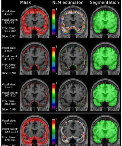
are propagated and processed at a higher resolution (Vj−k+1). This procedure is repeated until the resolution of the stereotaxic space Vj is reached. In this manner, the initialization mask of each resolution step is limited to the voxels with uncertain segmentation at the previous step (Fig. 3). This greatly reduces the computational cost. At the stereotaxic resolution, segmentation is done by thresholding the estimator vVj(xi) at 0.5.
During experiments, we used three resolutions (k = 2) with isotropic voxel spacing respectively of 4 mm, 2 mm, and 1 mm (stereotaxic space resolution) (see Fig. 3). We empirically chose
confidence level α and variable patch size and search area depending on the resolution (see Table 1).
Voxel size (mm3) Patch size (voxels) Search area (voxels) α
4×4×4 3×3×3 3×3×3 0.2
2×2×2 3×3×3 9×9×9 0.2
1×1×1 5×5×5 13×13×13 -
Table 1. Patch size, search area, and confidence level α chosen for the three resolutions
4. Validation
In our validation of the proposed method we used the Dice similarity coefficient (DSC) (Dice, 1945) adapted to binary images when comparing to the gold standard brain segmentations described above. The DSC is defined as | | | | | |, where A is the set of voxels in the proposed segmentation and B is the set of voxels in the reference segmentation and |∙| is the cardinality. Furthermore, we calculated the false positive rate (FPR) as | |
| | and the false negative rate
(FNR) as | |
| |, where FP is the set of false positive voxels, TN the set of true negative voxels,
FN the set of false negative voxels, and TP the set of true positive voxels.
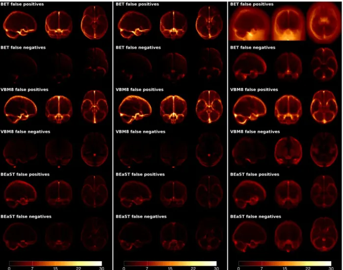
To visualize errors, we generated false positive and false negative images for each segmentation using the gold standard. These error images were averaged and the resulting image intensities were projected onto the three principal planes (axial, coronal, sagittal) using mean intensity projection in a manner similar to that done in Segmentation Validation Engine (Shattuck et al., 2009).
4.1 Leave-one-out cross validation
To evaluate the robustness and the accuracy of BEaST, we measured the segmentation accuracy in a leave-one-out cross validation (LOOCV) fashion. Each of the 80 library images was processed with the remaining 79 images as priors (158 after mid-sagittal flipping), and the resulting segmentation was compared to the manually corrected labels in the library. In this
experiment, we varied the number of selected priors from the library to evaluate the impact of N on segmentation accuracy. During our experiment, N varied from 2 to 40.
4.2 Comparison to other methods
A comparison to BET (Smith, 2002) and VBM8 (http://dbm.neuro.uni-jena.de/vbm/download) was performed. We chose to compare with BET, as BET is publicly available, widely used, and has been shown to perform well in several recent brain extraction comparisons (Carass et al., 2011; Iglesias et al., 2011; Leung et al., 2011). The choice of VBM8 was based on its availability and the fact that it is the highest-ranking publicly available method in the archive of the online Segmentation Validation Engine for brain segmentation (Shattuck et al., 2009) (http://sve.loni.ucla.edu/archive/).
BET iteratively deforms an ellipsoid mesh, initialized inside the brain, to the GM/CSF boundary. The target of BET is very similar to our definition of the optimal brain segmentation (see Section 2). We used BET version 2.1 from FSL version 4.1. Since BET performs better with robust brain center estimation and when the neck is not visible in the image (Iglesias et al., 2011), we applied BET on the normalized and stereotaxically aligned images with default parameters.
VBM8 performs the brain extraction by thresholding the tissue probability map in stereotaxic space, generated using the SPM framework (Ashburner, 2007; Ashburner and Friston, 2009), and followed by repeated morphological openings to remove non-brain tissues connected by thin bridges. We used release 419 of VBM8, which was the latest version by the time of writing. By experiments, we found that VBM8 provided better results when initialized with native images in contrast to stereotactically registered images. In order to perform the best fair comparison, this method was thus applied in native space.
BET and VBM8 were applied on the entire library of scans and DSCs, FPRs, and FNRs were calculated using the gold standard segmentations.
4.3 Independent validation
Comparing the results of BEaST to gold standard segmentations, which are also used as priors, a bias may be introduced that affect the results in favour of BEaST. Such a comparison effectively demonstrates that the method can provide results similar to our definition. However, when
comparing to methods with no priors, a bias is introduced. Therefore, we performed validation using an independent test set available in the online Segmentation Validation Engine (SVE) of brain segmentation methods (Shattuck et al., 2009). The test set consists of 40 T1w MRI scans (20 males and 20 females; age range 19 - 40). The web service allows the comparison of results with hand-corrected brain masks. The DSC, sensitivity (SEN), and specificity (SPE) are calculated automatically, where SEN and SPE are related to FNR and FPR by: SEN=1 - FNR and SPE=1 - FPR. The web service contains an archive of all uploaded results, which enables segmentation methods to be objectively benchmarked and compared between each other.
4.4 Robustness
Finally, we evaluated the robustness of BEaST, and compared it to BET, by applying the method to all 1.5T T1w baseline ADNI data (200 AD, 408 MCI, and 232 CN). A strict manual quality control procedure was carried out to label the results “pass” or “fail” corresponding to whether the individual brain mask met the definition given in Section 2 and whether the mask was sufficient for further processing in a cortical surface analysis study. Masks from BEaST and BET were rated in a blinded fashion (i.e., the rater did not know which of the 1680 masks came from which procedure. This way, the failure rate of BEaST was compared to the failure rate of BET on the same data. A comparison to BET was chosen as BET demonstrated better compliance with our brain mask definition (see Section 2) than VBM8 during our validation experiments.
5. Results
5.1 Leave-one-out cross validation
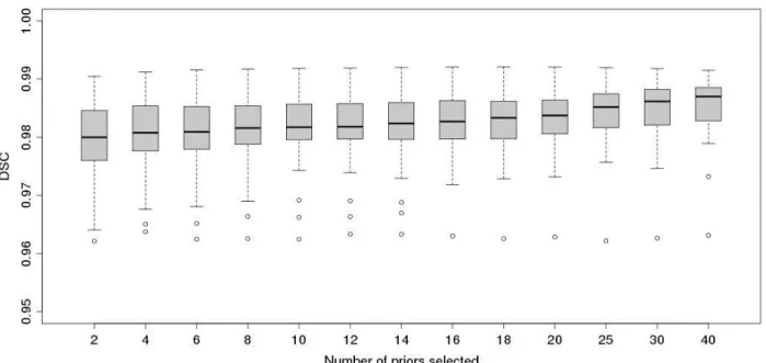
Figure 4 shows the DSCs for increasing number of priors selected from the library when compared to the gold standard. As shown in Coupé et al. (2011), increasing the number of selected priors improves the segmentation accuracy with the average DSC increasing from 0.9797 (N=2) to 0.9856 (N=40). In our experiment, accuracy is high even when using only very few selected priors. Increasing the number of selected priors appears to make the segmentations more consistent as the standard deviation is reduced from 0.0072 (N=2) to 0.0049 (N=40). The results show a single persistent outlier that does not benefit from increasing N. This outlier is the segmentation of the youngest (age=6y) subject in the dataset. The remaining NIHPD subjects in
the dataset are aged from 7y to 18y. This suggests that the maturation of the brain and skull alters the structural appearance in the T1w scans. Thus, the structural redundancy of the “youngest scan” is low within the library, and increasing N does not increase the number of similar patches.
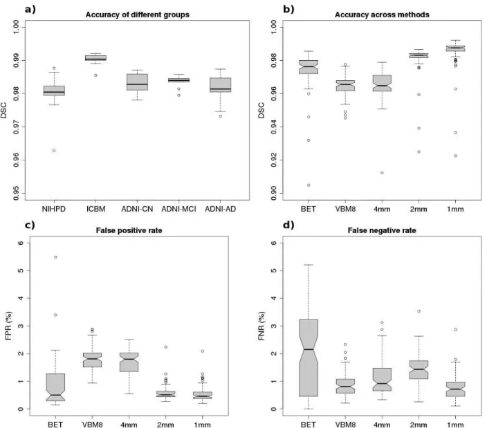
Though the experiment showed an increase of accuracy with increasing N, we chose N=20 for further experiments as the higher accuracy comes at a cost of longer computation time. Figure 5a shows the segmentation accuracy within the different groups used in the experiments for N=20. With an average DSC of 0.9901, the accuracy on ICBM data is significantly higher (p<0.001, two-tailed t-test) than the accuracy of the other groups tested. This may be due to the fact that the 10 ICBM data sets evaluated here were acquired on a single scanner, and thus are more homogeneous than the other groups, which lead to higher redundancy and better matches of patches during the segmentation process for this group of example data.
5.2 Comparison to other methods
In Table 2, the DSC, FPR, and FNR are provided for BET, VBM8, and BEaST (N=20) when tested on the three different datasets used in our study. BET yielded very high DSC for ICBM and NIHPD, while the results are more mixed on ADNI as indicated by the high standard deviation and the increased rates of false positives and false negatives. VBM8 provided slightly lower DSC on ICBM and NIHPD with similar FPR and FNR distributions, which are visualized in Fig. 6. On the ADNI dataset, VBM8 provided on average DSC values larger than those obtained by BET and is more consistent in its segmentation. In fact, VBM8 never results in catastrophic segmentations, which BET has a tendency to do from time to time (this can be observed on the false positives map in Fig. 6c, top row). BEaST yielded consistently high DSC on all data with generally balanced FPR and FNR that were significantly lower than the other methods except for the FNR on ICBM and ADNI, where VBM8 provides similar FNR values.
Table 2. Average DSC, FPR, and FNR for the methods tested on the different data sets used. The best results from each column are underlined. Two bottom rows: p-values for two-tailed paired
t-test comparing BEaST and respectively BET and VBM8. Significant (p<0.05) results are shown in italic and highly significant (p<0.01) results are shown in bold.
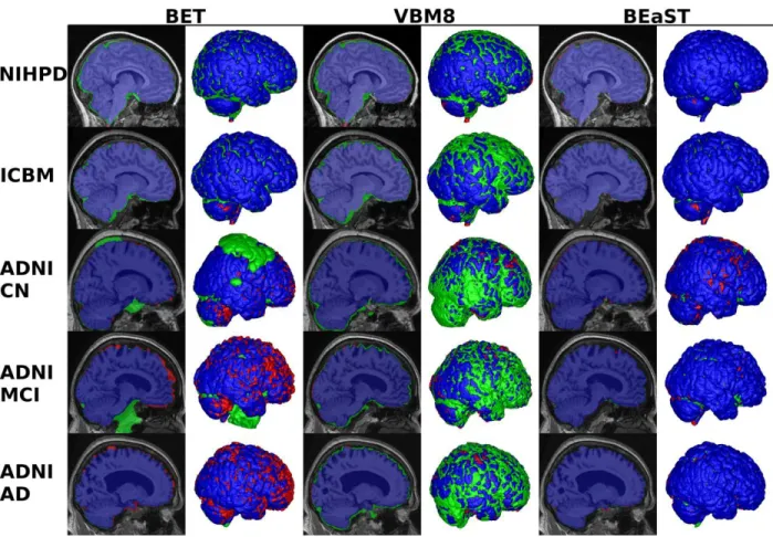
Figure 7 shows typical examples of brain masks obtained by BET, VBM8 and BEaST on the five different groups tested here (NIHPD, ICBM, ADNI-CN, ADNI-MCI, ADNI-AD). On NIHPD and ICBM data, BET behaved quite well with only minor segmentation errors, such as inclusion of the transverse sinus and part of the eye sockets. On ADNI data, more serious errors were found using BET. These include inclusion of dura and marrow of the skull while gyri are often cut off in atrophic brains. VBM8 had a tendency to perform over-segmentations on all groups and sometimes included dura proximate to the brain, carotid arteries, ocular fat / muscle, and parts of the eyes. On the positive side, VBM8 rarely removes part of the brain due to the consistent over-segmentation (see Fig. 6). BEaST generally provided a more consistent and robust segmentation without serious errors.
Figure 5b-d show the resulting DSCs, FPRs, and FNRs of BEaST compared to BET and VBM8. We measured the segmentation output for BEaST at each resolution by thresholding the nonlocal means estimator at 0.5. As shown, the accuracy increases along with scale, and at 2 mm voxel sizes (requiring about 1.25 min) BEaST has already significantly (p=0.01, paired t-test) higher median (and mean) accuracy than BET (Fig. 5b). The difference in DSCs between the techniques may seem small. However, when measuring DSC in the context of whole brain segmentations, small changes in the coefficient correspond to large changes in volume as demonstrated in (Rohlfing et al., 2004). In our case a change of 0.01 in DSC corresponds to about 30-40 cm3
ICBM NIHPD ADNI
Method DSC FPR % FNR % DSC FPR % FNR % DSC FPR % FNR % BET 0.975±0.003 1.28±0.22 0.45±0.13 0.975±0.003 1.33±0.15 0.24±0.05 0.944±0.115 3.81±12.7 2.71±1.25 VBM8 0.967±0.002 1.69±0.13 0.55±0.07 0.972±0.003 1.32±0.21 0.84±0.23 0.963±0.005 1.88±0.43 0.92±0.46 BEaST 0.990±0.002 0.41±0.12 0.49±0.12 0.981±0.005 1.02±0.27 0.20±0.07 0.985±0.011 0.53±0.40 0.91±0.40
BEaST compared to other methods (p-values)
BET 1.44×10⁻⁸ 9.39×10⁻⁸ 3.28×10⁻¹
2.59×10⁻⁴ 4.43×10⁻⁴ 4.62×10⁻²
6.66×10⁻³ 5.01×10⁻²
2.19×10⁻¹⁵
depending on brain size and the false positives - false negatives ratio. This volume is relatively large when compared to the size of the structures, which are usually measured in neuroimaging studies (e.g.; the size of the human hippocampus is about 3.5 cm3). The varying bias of the DSC when segmenting structures of different sizes (Rohlfing et al., 2004) in our case is considered low, as the brains have been spatially normalized. The FPRs and FNRs shown in Fig. 5c-d illustrate the large effect of a small difference in DSC. Compared to VBM8, the FPR is reduced by 74% using BEaST, and FNR is reduced by 67% compared to BET. Because of the consistent over-segmentation, VBM8 has an FNR similar to BEaST at the highest resolution. Even though the results of BET have a similar median FPR compared to the FPR of BEaST, the FPR of BET is significantly (p=0.05) different from the FPR of BEaST.
5.3 Independent Validation
Images from the independent test dataset from the Segmentation Validation Engine were normalized in the same way as the library images. Validation of BEaST (N=20) using the test dataset resulted in a mean DSC of 0.9781±0.0047 with FPR of 1.13%±0.35% and FNR of 0.60%±0.25% (see http://sve.loni.ucla.edu/archive/study/?id=244). At the time of writing, this result was the best of all the methods published on the website. MAPS had a second place with a DSC of 0.9767±0.0021 followed by VBM8 with a DSC of 0.9760±0.0025. When compared with BEaST, the differences in results with these two other techniques are statistically significant (p<0.03, paired t-test).
5.4 Robustness
After careful, blinded quality control of the 2×840 baseline ADNI data volumes from BEaST
(N=20) and BET, 599 images processed with BEaST were found to be acceptable for further
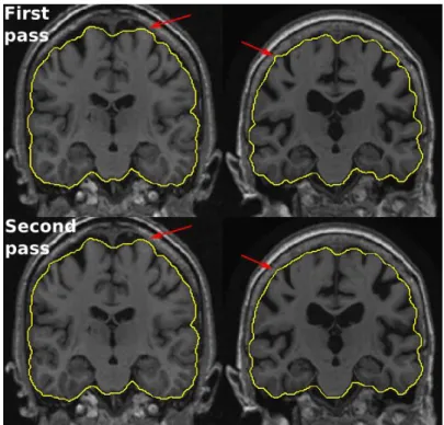
cortical surface analysis while only 125 images processed with BET were acceptable. This corresponds to a failure rate of 29% for BEaST and 85% for BET. Figure 8 shows examples of segmentations that failed the quality control. As seen from the figure, if any part of the cortex was removed or any part of the dura was included by the segmentation, the result was rejected. Performing a second pass with BEaST (N=20) using the 599 accepted segmentations with corresponding images as priors, and re-applying BEaST (with the subject's MRI left out of the
template library) the failure rate was reduced to 10% corresponding to 86 scans (see Fig. 8 for examples of improvements after second pass). Many of these persistently failing scans had motion or Gibbs ringing artifacts, and some had parts of the brain present outside the initialization mask. No catastrophic errors were detected and the manual corrections needed for passing the brain masks were small. In fact, for other types of analyses, such as segmentations of deep brain structures, all brain masks produced by BEaST would pass the quality control.
5.5 Computation time
In our experiments, with 20 images selected from the template library, the total processing time using a single thread on an Intel Core i7-950 processor at 3.06 GHz was less than 30 min per subject. With 10 images, the processing time was less than 20 min per subject. By contrast, without the multi-resolution step, but using the initialization mask, the processing time was around 320 min. Removing the initialization mask increased the processing time to 42 h. The average processing times of BET and VBM8 were about respectively 2.5 min and 12 min, including the spatial and intensity normalization. Obtaining the segmentation of BEaST at 2 mm voxel sizes takes about 2 min including the spatial and intensity normalization, and the corresponding DSCs are significantly (p<0.03) higher than either BET or VBM8 (Fig. 5b). This suggests that a fast low-resolution result may be available for certain analyses that do not require a highly detailed mask. Compared to MAPS, which yields similar accuracy as BEaST, the processing time of BEaST is about 40 times shorter on similar hardware.
6. Discussion
The leave-one-out cross-validation showed that the segmentation accuracy is consistently high (average DSC for N=20: 0.9834±0.0053) and that selecting more priors from the library increase the accuracy. However, there is a trade-off between the number of selected priors and segmentation accuracy, why we chose to set N=20 for our validation. The results showed a higher accuracy on ICBM data compared to the other groups tested. This may be caused by the fact that i) all ICBM images were acquired using the same scanner, and ii) the anatomical variability within this group may be smaller than the other groups studied. This suggests that the accuracy may be improved by extending the number of priors for the groups with higher
anatomical variability and multi-site acquisitions. Although the results show that only a relatively small library is needed, the library still needs to be representative of all the data for the patch-based segmentation to work optimally.
The excellent results on ICBM and NIHPD suggest that using an unbalanced library of priors does not impair the segmentation accuracy of the data, which is underrepresented in the library. We used only 10 priors from each of these databases in the library, while using 60 priors from the ADNI database. The template pre-selection seems sufficiently robust to select the appropriate priors.
The chosen patch sizes and search areas seem appropriate for segmenting the brain. The choice of α=0.2 was chosen empirically. Generally, the choice of α can be viewed as a trade-off between computation time and segmentation accuracy. However, performing the segmentations only at the highest resolution may result in false positives as illustrated in Fig. 3, bottom row. Thus, the aim of the low resolution segmentation is to exclude dura and other tissues with similar intensity compositions as those found within the brain. We found that setting α=0.2 consistently achieved this.
6.1 Comparison to publicly available methods
Our comparison to other popular brain extraction methods showed that BET and VBM8 provides very good results for scans of normal individuals, while pathological data seems to impose a problem for these methods. BET has widely been the preferred brain extraction method for almost 10 years, and for many purposes BET is still sufficient. The simplicity of the method without the need for priors or registration is appealing. However, the emergence of large databases with thousands of images with and without pathology calls for flexible and robust brain extraction methods. This can be achieved by using label fusion methods as demonstrated in (Leung et al., 2011) and our study.
Testing on all baseline ADNI data demonstrated that BEaST reduced the failure rate from 85% to 29% when compared to BET. These high failure rates were caused by a very strict quality
control, where a brain segmentation was discarded if any error according to the definition (Section 2) was discovered. A failure rate of 29% is still unacceptable. However, after a second pass, where the accepted segmentations were included into the library of priors, the failure rate was reduced to 10%, which is acceptable as the manual corrections needed are small. A third pass may have passed a few more brain masks. However, as the errors seemed to stem from either image artifacts or insufficient initialization mask (or insufficient linear registration), a third pass was not attempted. Learning from priors enables iterative procedures (boot-strapping) for propagating the segmentation definition, where low failure rates can be obtained. This cannot be achieved by segmentation methods without priors, such as BET and VBM8.
Compared to BET and VBM8, BEaST produced less than half of the segmentation errors, increasing the average DSC from respectively 0.9522 and 0.9647 to 0.9834. In terms of speed, BET is faster than BEaST, if the segmentations are performed at the highest resolution. However, stopping the processing at 2 mm voxel sizes results in computation times similar to BET, while still obtaining significantly (p=0.01, paired two-tailed t-test) higher segmentation accuracy. Compared to the combined atlas and morphological approach in VBM8, BEaST yields superior segmentation results on all data tested in the study. The error maps (Fig. 6) show that VBM8 consistently oversegments the brain compared to our definition. BET behaves similarly, but with less over-segmentations. To be fair, such segmentations may be useful in many cases and thus should not be considered as erroneous. However, for the application of cortical surface analysis, it is crucial to not include proximate dura in the brain segmentation, as this may lead to over-segmentations of the cortex and in turn to overestimations of cortical thickness (van der Kouwe et al., 2008).
A limitation of the quantitative comparison is that the DSC does not necessarily say anything about whether the resulting segmentation is sufficient for the subsequent processing. For example, many false negatives may be due to only removing CSF from the surface of the brain compared to the gold standard. As such, these discrepancies are not fatal errors for the subsequent processing.
The high DSC of BEaST compared to VBM8 and BET in the LOOCV can be explained by the fact that BEaST learns from the priors, while the other methods have no segmentation priors. This means that BEaST delivers segmentations we can expect to match the definition, while this is not the case for BET and VBM8. Thus the results of BEaST are biased toward the segmentations of the priors and the DSC may be artificially high in the LOOCV. That is why the independent validation using the SVE was necessary.
The bias toward the priors illustrates the flexibility of the patch-based approach. If another definition is needed, the right priors just need to be available for BEaST to provide consistent segmentations on new data. This is also a limitation of BEaST in its current form. While other pathologies, which do not significantly change the appearance of the brain tissues, such as fronto-temporal dementia, should be consistently segmented with the current library of BEaST, other pathologies, such as tumors and lesions, may impose a problem for the segmentation. Over time, a library representative for the large variety of brains may be constructed to overcome this limitation in the future.
6.2 Comparison to state of the art
In terms of Dice overlap, results obtained by BEaST are better than those reported from recent hybrid brain extraction approaches (Carass et al., 2011; Iglesias et al., 2011) and similar to those from a label fusion approach, MAPS (Leung et al., 2011). In the label fusion approach, the library is more than 10 times larger and the processing time about 40 times longer. The short processing time in BEaST (<30 min) results from only needing linear registrations and the advantage of using the ROI in the multi-resolution strategy. The current implementation runs as a single thread. However, the nonlocal means calculations can easily be parallelized and implemented to exploit the common multi-core CPUs and even GPU processing (Palhano Xavier de Fontes et al., 2011), which will decrease processing time significantly, possibly making it close to real time.
Using the online segmentation validation engine (Shattuck et al., 2009) we obtained a truly objective measure of the performance of BEaST. A mean DSC of 0.9781 is significantly
(p=0.03, paired t-test) better than the best score by MAPS (0.9767). An advantage of the nonlocal means approach is the possibility to use the redundancy in the image priors. While conventional label fusion approaches provide a one-to-one mapping between the image under study and the image priors, the nonlocal means approach provides a one-to-many mapping to support the segmentation decision at each voxel. That is why a relatively small number of library priors are needed in the patch-based segmentation compared to conventional label fusion approaches. This makes it feasible to distribute the method as downloadable software. We intend to make BEaST available online (http://www.bic.mni.mcgill.ca/BEaST) including the library if permission to redistribute the data can be obtained.
As in conventional label fusion, the nonlocal means approach enables the segmentation of different targets simultaneously. For example, the intracranial cavity may be obtained by generating priors using appropriate methods, such as the multi-modal approach used as intermediate step to obtain the brain segmentation priors for the ICBM and NIHPD datasets. Also, separation of cerebellum and brain stem from the cerebrum may be achieved with high accuracy if the appropriate structural priors are available.
Recent work by Wang et al. (2011) showed that several segmentation algorithms perform systematic errors, which can be corrected using a wrapper-based learning method. In the study, BET was used to demonstrate the wrapper-based approach, which improved the average DSC from 0.948 to 0.964. This similarity is still lower than the average similarity obtained by BEaST. There are no indications that the accuracy of BEaST can be improved using the wrapper-based learning approach, as the error maps of BEaST show no systematic error (Fig. 6). The false positives and false negatives are uniformly distributed across the brain. The segmentations of VBM8 may benefit from the wrapper approach, as these exhibit consistent over-segmentations.
All images used in this study were acquired using scanners with 1.5T field strengths. Though the results demonstrated robustness towards multi-site acquisition, the sensitivity to scanner field strength remains to be investigated. As shown in (Keihaninejad et al., 2010), the scanner field strength has significant impact on intra-cranial cavity segmentations. A similar effect can be
expected for brain extractions. However, our results indicate that extending the library with appropriate templates (in this case images from 3T scanners) may deal with a potential bias. This is supported by the results obtained by MAPS (Leung et al., 2011) on data from scanners with 1.5T and 3T field strengths.
7. Conclusion
In conclusion, we have proposed a new brain extraction method, BEaST, based on nonlocal segmentation embedded within a multi-resolution framework. The accuracy of the method is higher than BET, VBM8, and recent hybrid approaches and similar to that of a recent label fusion method MAPS, while being much faster and requiring a smaller library of priors. Using all baseline ADNI data, the study demonstrated that the nonlocal segmentation is robust and consistent if the right priors are available.
Acknowledgements
The authors would like to thank Professor Nick Fox, Dementia Research Centre, Institute of Neurology, London, for contributing with the ADNI semi-automatic brain segmentations. This work has been supported by funding from the Canadian Institutes of Health Research MOP-84360 & MOP-111169 as well as CDA (CECR)-Gevas-OE016. KKL acknowledges support from the MRC, ARUK and the NIHR. The Dementia Research Centre is an Alzheimer's Research UK Co-ordinating Centre and has also received equipment funded by the Alzheimer's Research UK. This work has been partially supported by the Spanish Health Institute Carlos III through the RETICS Combiomed, RD07/0067/2001.
The authors recognize the work done by Professor Steve Smith and Dr. Christian Gaser for making respectively BET and VBM8 available to the neuroimaging community.
Data collection and sharing for this project was funded by the Alzheimer's Disease Neuroimaging Initiative (ADNI) (National Institutes of Health Grant U01 AG024904). ADNI is funded by the National Institute on Aging, the National Institute of Biomedical Imaging and Bioengineering, and through generous contributions from the following: Abbott, AstraZeneca AB, Bayer Schering Pharma AG, Bristol-Myers Squibb, Eisai Global Clinical Development,
Elan Corporation, Genentech, GE Healthcare, GlaxoSmithKline, Innogenetics, Johnson and Johnson, Eli Lilly and Co., Medpace, Inc., Merck and Co., Inc., Novartis AG, Pfizer Inc, F. Hoffman-La Roche, Schering-Plough, Synarc, Inc., as well as non-profit partners the Alzheimer's Association and Alzheimer's Drug Discovery Foundation, with participation from the U.S. Food and Drug Administration. Private sector contributions to ADNI are facilitated by the Foundation for the National Institutes of Health (www.fnih.org). The grantee organization is the Northern California Institute for Research and Education, and the study is coordinated by the Alzheimer's Disease Cooperative Study at the University of California, San Diego. ADNI data are disseminated by the Laboratory for Neuro Imaging at the University of California, Los Angeles. This research was also supported by NIH grants P30AG010129, K01 AG030514, and the Dana Foundation.
References
Aljabar, P., Heckemann, R., Hammers, A., Hajnal, J.V., Rueckert, D., 2007. Classifier selection strategies for label fusion using large atlas databases. Medical image computing and computer-assisted intervention : MICCAI ... International Conference on Medical Image Computing and Computer-Assisted Intervention 10, 523-531.
Ashburner, J., 2007. A fast diffeomorphic image registration algorithm. NeuroImage 38, 95-113. Ashburner, J., Friston, K.J., 2000. Voxel-based morphometry--the methods. NeuroImage 11, 805-821. Ashburner, J., Friston, K.J., 2009. Computing average shaped tissue probability templates. NeuroImage 45, 333-341.
Baillard, C., Hellier, P., Barillot, C., 2001. Segmentation of brain 3D MR images using level sets and dense registration. Medical image analysis 5, 185-194.
Boesen, K., Rehm, K., Schaper, K., Stoltzner, S., Woods, R., Luders, E., Rottenberg, D., 2004. Quantitative comparison of four brain extraction algorithms. NeuroImage 22, 1255-1261.
Buades, A., Coll, B., Morel, J.M., 2005. A Review of Image Denoising Algorithms, with a New One. Multiscale Modeling & Simulation 4, 490-530.
Carass, A., Cuzzocreo, J., Wheeler, M.B., Bazin, P.-L., Resnick, S.M., Prince, J.L., 2011. Simple paradigm for extra-cerebral tissue removal: Algorithm and analysis. NeuroImage 56, 1982-1992. Collins, D.L., Neelin, P., Peters, T.M., Evans, A.C., 1994. Automatic 3D intersubject registration of MR volumetric data in standardized Talairach space. Journal of computer assisted tomography 18, 192-205. Collins, D.L., Pruessner, J.C., 2010. Towards accurate, automatic segmentation of the hippocampus and amygdala from MRI by augmenting ANIMAL with a template library and label fusion. NeuroImage 52, 1355-1366.
Coupé, P., Manjón, J., Fonov, V., Pruessner, J., Robles, M., Collins, L., 2010. Nonlocal patch-based label fusion for hippocampus segmentation. Medical image computing and computer-assisted intervention : MICCAI ... International Conference on Medical Image Computing and Computer-Assisted Intervention 13, 129-136.
Coupé, P., Manjón, J., Fonov, V., Pruessner, J., Robles, M., Collins, L., 2011. Patch-based segmentation using expert priors: application to hippocampus and ventricle segmentation. NeuroImage 54, 940-954. Coupe, P., Yger, P., Prima, S., Hellier, P., Kervrann, C., Barillot, C., 2008. An optimized blockwise nonlocal means denoising filter for 3-D magnetic resonance images. Medical Imaging, IEEE Transactions on 27, 425-441.
Dale, A.M., Fischl, B., Sereno, M.I., 1999. Cortical surface-based analysis. I. Segmentation and surface reconstruction. NeuroImage 9, 179-194.
Dice, L.R., 1945. Measures of the Amount of Ecologic Association Between Species. Ecology 26, 297 - 302.
Eskildsen, S.F., Ostergaard, L.R., 2006. Active surface approach for extraction of the human cerebral cortex from MRI. Medical image computing and computer-assisted intervention : MICCAI ...
International Conference on Medical Image Computing and Computer-Assisted Intervention 9, 823-830. Evans, A.C., 2006. The NIH MRI study of normal brain development. NeuroImage 30, 184-202.
Fennema-Notestine, C., Ozyurt, I.B., Clark, C.P., Morris, S., Bischoff-Grethe, A., Bondi, M.W., Jernigan, T.L., Fischl, B., Segonne, F., Shattuck, D.W., Leahy, R.M., Rex, D.E., Toga, A.W., Zou, K.H., Brown,
G.G., 2006. Quantitative evaluation of automated skull-stripping methods applied to contemporary and legacy images: effects of diagnosis, bias correction, and slice location. Human brain mapping 27, 99-113. Fonov, V., Evans, A.C., Botteron, K., Almli, C.R., McKinstry, R.C., Collins, D.L., 2011. Unbiased average age-appropriate atlases for pediatric studies. NeuroImage 54, 313-327.
Goldszal, A.F., Davatzikos, C., Pham, D.L., Yan, M.X., Bryan, R.N., Resnick, S.M., 1998. An image-processing system for qualitative and quantitative volumetric analysis of brain images. Journal of computer assisted tomography 22, 827-837.
Hahn, H.K., Peitgen, H.-O., 2000. The Skull Stripping Problem in MRI Solved by a Single 3D Watershed Transform. Proceedings of the Third International Conference on Medical Image Computing and
Computer-Assisted Intervention. Springer-Verlag, pp. 134-143.
Hartley, S.W., Scher, A.I., Korf, E.S., White, L.R., Launer, L.J., 2006. Analysis and validation of automated skull stripping tools: a validation study based on 296 MR images from the Honolulu Asia aging study. NeuroImage 30, 1179-1186.
Heckemann, R.A., Hajnal, J.V., Aljabar, P., Rueckert, D., Hammers, A., 2006. Automatic anatomical brain MRI segmentation combining label propagation and decision fusion. NeuroImage 33, 115-126. Iglesias, J., Liu, C., Thompson, P., Tu, Z., 2011. Robust Brain Extraction Across Datasets and
Comparison with Publicly Available Methods. Medical Imaging, IEEE Transactions on 30, 1617-1634. Kapur, T., Grimson, W.E., Wells, W.M., 3rd, Kikinis, R., 1996. Segmentation of brain tissue from magnetic resonance images. Medical image analysis 1, 109-127.
Keihaninejad, S., Heckemann, R.A., Fagiolo, G., Symms, M.R., Hajnal, J.V., Hammers, A., 2010. A robust method to estimate the intracranial volume across MRI field strengths (1.5T and 3T). NeuroImage 50, 1427-1437.
Lee, J.M., Yoon, U., Nam, S.H., Kim, J.H., Kim, I.Y., Kim, S.I., 2003. Evaluation of automated and semi-automated skull-stripping algorithms using similarity index and segmentation error. Computers in biology and medicine 33, 495-507.
Lemieux, L., Hagemann, G., Krakow, K., Woermann, F.G., 1999. Fast, accurate, and reproducible automatic segmentation of the brain in T1-weighted volume MRI data. Magnetic resonance in medicine : official journal of the Society of Magnetic Resonance in Medicine / Society of Magnetic Resonance in Medicine 42, 127-135.
Leung, K.K., Barnes, J., Modat, M., Ridgway, G.R., Bartlett, J.W., Fox, N.C., Ourselin, S., 2011. Brain MAPS: an automated, accurate and robust brain extraction technique using a template library.
NeuroImage 55, 1091-1108.
Leung, K.K., Barnes, J., Ridgway, G.R., Bartlett, J.W., Clarkson, M.J., Macdonald, K., Schuff, N., Fox, N.C., Ourselin, S., 2010. Automated cross-sectional and longitudinal hippocampal volume measurement in mild cognitive impairment and Alzheimer's disease. NeuroImage 51, 1345-1359.
Manjon, J.V., Carbonell-Caballero, J., Lull, J.J., Garcia-Marti, G., Marti-Bonmati, L., Robles, M., 2008. MRI denoising using non-local means. Medical image analysis 12, 514-523.
Mazziotta, J.C., Toga, A.W., Evans, A., Fox, P., Lancaster, J., 1995. A probabilistic atlas of the human brain: theory and rationale for its development. The International Consortium for Brain Mapping (ICBM). NeuroImage 2, 89-101.
Mikheev, A., Nevsky, G., Govindan, S., Grossman, R., Rusinek, H., 2008. Fully automatic segmentation of the brain from T1-weighted MRI using Bridge Burner algorithm. Journal of magnetic resonance imaging : JMRI 27, 1235-1241.
Mueller, S.G., Weiner, M.W., Thal, L.J., Petersen, R.C., Jack, C., Jagust, W., Trojanowski, J.Q., Toga, A.W., Beckett, L., 2005. The Alzheimer's disease neuroimaging initiative. Neuroimaging clinics of North America 15, 869-877, xi-xii.
Nyul, L.G., Udupa, J.K., 2000. Standardizing the MR image intensity scales: making MR intensities have tissue-specific meaning. In: Mun, S.K. (Ed.). SPIE, San Diego, CA, USA, pp. 496-504.
Palhano Xavier de Fontes, F., Andrade Barroso, G., Coupé, P., Hellier, P., 2011. Real time ultrasound image denoising. Journal of Real-Time Image Processing 6, 15-22.
Park, J.G., Lee, C., 2009. Skull stripping based on region growing for magnetic resonance brain images. NeuroImage 47, 1394-1407.
Rehm, K., Schaper, K., Anderson, J., Woods, R., Stoltzner, S., Rottenberg, D., 2004. Putting our heads together: a consensus approach to brain/non-brain segmentation in T1-weighted MR volumes.
NeuroImage 22, 1262-1270.
Rex, D.E., Shattuck, D.W., Woods, R.P., Narr, K.L., Luders, E., Rehm, K., Stoltzner, S.E., Rottenberg, D.A., Toga, A.W., 2004. A meta-algorithm for brain extraction in MRI. NeuroImage 23, 625-637. Rohlfing, T., Brandt, R., Menzel, R., Maurer, C.R., Jr., 2004. Evaluation of atlas selection strategies for atlas-based image segmentation with application to confocal microscopy images of bee brains.
NeuroImage 21, 1428-1442.
Sabuncu, M.R., Balci, S.K., Shenton, M.E., Golland, P., 2009. Image-driven population analysis through mixture modeling. IEEE transactions on medical imaging 28, 1473-1487.
Sadananthan, S.A., Zheng, W., Chee, M.W., Zagorodnov, V., 2010. Skull stripping using graph cuts. NeuroImage 49, 225-239.
Sandor, S., Leahy, R., 1997. Surface-based labeling of cortical anatomy using a deformable atlas. IEEE transactions on medical imaging 16, 41-54.
Segonne, F., Dale, A.M., Busa, E., Glessner, M., Salat, D., Hahn, H.K., Fischl, B., 2004. A hybrid approach to the skull stripping problem in MRI. NeuroImage 22, 1060-1075.
Shan, Z.Y., Yue, G.H., Liu, J.Z., 2002. Automated histogram-based brain segmentation in T1-weighted three-dimensional magnetic resonance head images. NeuroImage 17, 1587-1598.
Shattuck, D.W., Prasad, G., Mirza, M., Narr, K.L., Toga, A.W., 2009. Online resource for validation of brain segmentation methods. NeuroImage 45, 431-439.
Shattuck, D.W., Sandor-Leahy, S.R., Schaper, K.A., Rottenberg, D.A., Leahy, R.M., 2001. Magnetic resonance image tissue classification using a partial volume model. NeuroImage 13, 856-876. Sled, J.G., Zijdenbos, A.P., Evans, A.C., 1998. A nonparametric method for automatic correction of intensity nonuniformity in MRI data. IEEE transactions on medical imaging 17, 87-97.
Smith, S.M., 2002. Fast robust automated brain extraction. Human brain mapping 17, 143-155. Smith, S.M., Jenkinson, M., Woolrich, M.W., Beckmann, C.F., Behrens, T.E., Johansen-Berg, H., Bannister, P.R., De Luca, M., Drobnjak, I., Flitney, D.E., Niazy, R.K., Saunders, J., Vickers, J., Zhang, Y., De Stefano, N., Brady, J.M., Matthews, P.M., 2004. Advances in functional and structural MR image analysis and implementation as FSL. NeuroImage 23 Suppl 1, S208-219.
van der Kouwe, A.J., Benner, T., Salat, D.H., Fischl, B., 2008. Brain morphometry with multiecho MPRAGE. NeuroImage 40, 559-569.
Wang, H., Das, S., Suh, J.W., Altinay, M., Pluta, J., Craige, C., Avants, B., Yushkevich, P., 2011. A learning-based wrapper method to correct systematic errors in automatic image segmentation:
consistently improved performance in hippocampus, cortex and brain segmentation. NeuroImage 55, 968-985.
Wang, Z., Bovik, A.C., Sheikh, H.R., Simoncelli, E.P., 2004. Image quality assessment: from error visibility to structural similarity. IEEE transactions on image processing : a publication of the IEEE Signal Processing Society 13, 600-612.
Ward, B.D., 1999. 3dIntracranial: Automatic segmentation of intracranial region.
Warfield, S.K., Zou, K.H., Wells, W.M., 2004. Simultaneous truth and performance level estimation (STAPLE): an algorithm for the validation of image segmentation. Medical Imaging, IEEE Transactions on 23, 903-921.
Zhuang, A.H., Valentino, D.J., Toga, A.W., 2006. Skull-stripping magnetic resonance brain images using a model-based level set. NeuroImage 32, 79-92.
Figures
Fig. 1. Construction of library priors using multiple modalities. A) Intensities from T1w, T2w, and PDw images are added. B) BET (Smith, 2002) is used to produce an ICC mask. C) FACE (Eskildsen and Østergaard, 2006) is used to delineate the cortical boundary and produce a cerebrum mask. D) Cerebellum and brain stem are added by stereotaxic masks, and the mask is manually corrected.
Fig. 2. Adaptation of library priors using deformable surface. A) Semi-automatic GM/WM mask as used by MAPS (Leung et al., 2011). B) Adapted mask generated by deforming a surface mesh to the boundary of the GM/WM mask and manually corrected.
Fig. 3. The multiresolution segmentation process (row 1-3) compared to a single resolution approach (row 4). Column 1: Initialization mask. Column 2: Nonlocal means (NLM) estimator map. Column 3: Segmentation by thresholding the NLM estimator and adding the intersection mask. Processing times are accumulated time from initialization. Notice the inclusion of dura in the single resolution approach.
Fig. 4. Box-whisker plot of Dice similarity coefficient of segmentations using an increasing number of priors from the library. Experiment performed by leave-one-out using the library of 80 priors (10 NIHPD, 10 ICBM, 60 ADNI). The boxes indicate the lower quartile, the median and the upper quartile. The whiskers indicate respectively the smallest and largest observation excluding the outliers. Observations deviating more than two standard deviations from the mean are considered outliers and are marked as circles.
Fig. 5. a) Accuracy of BEaST segmentation within groups measured using Dice similarity coefficient. b) Segmentation accuracy measured at varying voxel sizes with BEaST compared to accuracy of BET and VBM8. c) False positive rate and d) false negative rate for BET, VBM8, and BEaST at varying voxel sizes. The notches in the box-whisker plots indicate the interquartile range and suggest statistically significant difference between the medians where the notches do not overlap.
Fig. 6. False positive and false negative maps for BET, VBM8, and BEaST on NIHPD, ICBM and ADNI data. All the error maps are displayed with the same scale. BET provided errors mainly located in the cerebral falx and medial temporal lobe structures. On the ADNI data, BET had a few catastrophic failures, which is visible in the false positive image. VBM8 tended to produce a systematic over-segmention compared to the used manual gold standard. The errors obtained by BEaST were more uniformly distributed indicating non-systematic segmentation errors.
Fig. 7. Typical results using BET, VBM8 and BEaST on the five test groups. The figure shows sagittal slices and 3D renderings of the segmentations. Column 1-2: BET segmentation. Column 3-4: VBM8 segmentation. Column 5-6: BEaST segmentation. Blue voxels are overlapping voxels in the segmentation compared to the gold standard. Green voxels are false positives and red voxels are false negatives.
Fig. 8. Examples of ADNI brain masks produced by BEaST not passing the quality control in the first pass (first row) and passing the quality control after second pass (second row). Left segmentation is discarded due to cortex clipping, while right segmentation is discarded due to inclusion of dura as indicated by the arrows. After second pass these errors are removed.