Design and implementation of a relative state estimator for docking and formation control of modular autonomous spacecraft

Design and Implementation of a Relative

State Estimator for Docking and Formation

Control of Modular Autonomous Spacecraft

by

Nicholas R. Hoff

iii

Submitted to the Department of Aeronautics and Astronautics

in partial fulfillment of the requirements for the degree of

Master of Science

at the

MASSACHUSETTS INSTITUTE OF TECHNOLOGY

June 2007

@

Massachusetts Institute of Technology 2007. All rights reserved.

A u th o r ...

...

... ...

Department of Aeronautics and Astronautics

May 25, 2007

Certified by ...

David W. Miller

Professor of Aeronautics and Astronautics

Thesis Supervisor

Accepted by...

Jaime Peraire

JUL 1

12007

Professor of Aeronautics and Astronautics

Chair, Committee on Graduate Students

Design and Implementation of a Relative

State Estimator for Docking and Formation

Control of Modular Autonomous Spacecraft

by

Nicholas R. Hoff

iii

Submitted to the Department of Aeronautics and Astronautics

on May 25, 2007, in partial fulfillment of the

requirements for the degree of

Master of Science

Abstract

Modularity is a promising design concept for space systems. In a modular satellite, the

individual subsystems would be broken down into physically distinct modules, which

would then dynamically recombine into an aggregate vehicle. This could improve the

flexibility and reusability of satellites, and could even enable some mission objectives

which are not possible at all with monolithic vehicles. However, modularity requires

that some additional new elements be included in the design that are not needed with

a monolithic satellite. Two of these are a docking interface to allow modules to attach,

and a position measurement system to allow modules to fly accurately in formation

and dock with each other. These two additional elements are explored in this thesis.

The central focus is on a relative state estimator based on an extended Kalman filter.

The estimator is first presented theoretically, then the results of implementation and

hardware testing are discussed. This thesis presents two main hardware applications

for the estimator, both of which mirror prime space-based applications of modularity

itself: docking and formation maintenance/reconfiguration.

Thesis Supervisor: David W. Miller

Title: Professor of Aeronautics and Astronautics

Acknowledgments

Parts of this work were funded by NASA MSFC under Award

#

01-44-49-001. We

are thankful for their support.

Several fellow graduate students in the Space Systems Lab at MIT were

invalu-ably helpful during this work. Simon Nolet, on whose work most of my work is

based, answered my endless questions about estimation on SPHERES and was

ex-tremely helpful throughout. Alvar Saenz-Otero was also invaluable in running tests

on SPHERES and SPHERES-related hardware, and spent many hours with us

work-ing on the electronics for SWARM. My colleague Swati Mohan was an instrumental

partner in the SWARM and SIFFT projects. Lennon Rodgers was a partner in the

design and fabrication of the UDP, discussed in Chapter 2. My advisor David W.

Miller provided technical suggestions and direction for this work, I am thankful to

him for letting me work in his lab. The team at the Flight Robotics Laboratory at

NASA MSFC was helpful with the SWARM and SIFFT testing described in Chapter

4, we thank them for letting us use their floor. Steve Sell and Chris Krebs of

Pay-load Systems Inc. have been helpful in creating high-quality mechanical designs and

fabricating high-quality hardware for us. The SPHERES project itself began as an

undergraduate design course, and credit for the current SPHERES satellites goes to

all the students who have worked on it over the years.

Lastly, I am so grateful to my mother for her endless love and support. It is the

only thing that I can count on absolutely, and it has made everything possible.

To my grandfather

An engineer

Contents

1 Introduction 15

1.1 M otivation . . . . 15

1.2 O verview . . . . 17

2 Universal Docking Port (UDP) 19 2.1 UDP Requirements ... ... 19 2.2 UD P Design . .. . . . .. . . . . 20 2.3 Estimation Hardware ... 24 2.4 Conclusion . . . . . 25 3 Relative Estimator 27 3.1 Architecture Choices . . . . 27 3.2 Available Measurements . . . . 28

3.3 State Vector and Attitude Representation . . . . 30

3.4 EKF Process - Linear Case . . . . 31

3.5 N onlinearities . . . . 34

3.5.1 Nonperiodic Measurements . . . . 35

3.5.2 Nonlinear Measurements . . . . 36

3.6 P refilter . . . . 41

3.7 C onclusion . . . . 42

4 Results and Applications 43 4.1 Testing of Ultrasound Receivers . . . . 43

4.2 Testing in Simulation . . . .

47

4.3 Hardware . . . .

50

4.3.1

SPHERES Satellites . . . .

53

4.3.2

Air Carriages . . . .

55

4.3.3

Avionics Stack . . . .

56

4.3.4

UDPs, Subapertures, and Other Hardware . . . .

57

4.3.5

Flat Table . . . .

57

4.4 SW ARM . . . .. . . . . .. . . . . 58

4.4.1

Setup . . . .

59

4.4.2

Experimental Plan . . . .

60

4.4.3

Sample Docking Results . . . .

61

4.4.4

Overall Docking Results . . . .

64

4.4.5

Reconfiguration Results . . . .

65

4.5 SIFFT . . . .

65

4.5.1

Hardware Setup . . . .

66

4.5.2

Estimation Configuration . . . .

66

4.5.3

Test plan . . . .

67

4.5.4

Results with Module 1 Fixed . . . .

69

4.5.5

Results with Rotation of Module 1 . . . .

69

4.6 Conclusion . . . .

71

5 Future Work and Conclusions 73

5.1

Future Work . . . .

73

5.1.1 UDPs use Beacons and Receivers . . . . 73

5.1.2 Star Tracker Mode . . . . 78

5.1.3 Full Global . . . . 82

5.1.4 Use Thruster Commands and Accelerometers . . . . 83

5.2 Conclusion . . . . 85

A Selected Code Segments 87

A.1 Overall Estimator Cycle . . . .

87

A.2 pads-stateUSBeaconDetPvarEKF() . . . . 89

A.3 pads hgenUSBeaconUpdatePvarEKF() . . . . 91

A .4 Qrot () . . . . 93

B Quaternion Attitude Representation 95

B. 1 Quaternion Composition and Properties . . . . 95

B.2 Quaternion Propagation . . . . 98

List of Figures

2-1 CAD drawing of a mostly-assembled UDP . . . . 21

2-2 CAD drawing of the UDP locking mechanism . . . . 22

2-3 CAD drawing of the UDP ring counterrotation mechanism . . . . 24

2-4 CAD drawing of the UDP with metrology rings in place . . . . 25

2-5 A picture of the front face of a fully assembled UDP . . . . 26

3-1 Timing diagram for ultrasound and infrared sensors . . . . 30

3-2 Update/Propagate diagram of an EKF . . . . 32

3-3 Basic cycle of a linear Kalman filter . . . . 33

3-4 Propagate/Update diagram of an EKF . . . . 35

3-5 Diagram showing nonlinearity in beacon-receiver separation measure-m ents . . . . 36

3-6 Notation of beacon and receiver positions in chaser and target reference fram es . . . . 37

4-1 60 seconds of raw data from one beacon-receiver pair . . . . 44

4-2 60 seconds of raw data from one beacon-receiver pair, zoomed in . . . 45

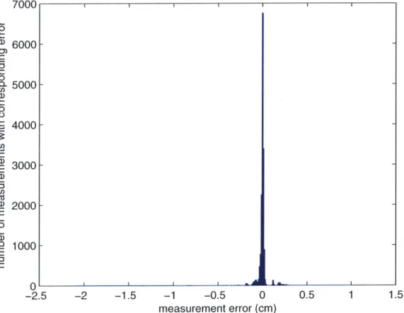
4-3 Histogram showing all Tij. from beacon-receiver pairwise tests . . . . 48

4-4 Relative estimator simulation,

o

4-5 Relative estimator simulation, ko

. . . .

52

4-6 A single SPHERES satellite . . . . 53

4-7 The SPHERES expansion port . . . . 54

4-8 A single puck air carriage . . . . 55

4-9 The avionics stack . . . . 56 11

4-10

4-11

4-12

4-13

4-14

4-15

4-16

4-17

4-18

4-19

The telescope aperture . . . .

The flat table in the MIT SSL . . . .

The SWARM tug module . . . .

The SWARM subaperture module . . . .

Data from a docking maneuver at MSFC . . . .

Data from a docking maneuver at MSFC . . . .

The SIFFT hardware setup . . . .

SIFFT estimation configuration and UDP field-of-view

A SIFFT formation reconfiguration test . . . .

A SIFFT formation reconfiguration test with rotation .

5-1 Notation of beacon and receiver positions in chaser and target reference

fram es . . . .

5-2 A possible measurement reordering . . . .

5-3 An external beacon . . . .

5-4 Beacon/receiver arrangement for the star tracker mode . . . .

5-5 Position/attitude coupling with single beacon star tracker . . . .

12 . . . . 57

. . . .

58

. . . .

59

. . . .

60

. . . .

62

. . . .

63

. . . .

66

. . . .

68

. . . .

70

. . . .

72

74

76

79

79

81

List of Tables

4.1 Summary of results from single beacon-receiver pair test. . . . . 46 4.2 Summary of results from all beacon-receiver pairs. . . . . 47

Chapter 1

Introduction

1.1

Motivation

The exploration, development, and use of space is limited by the complexity of oper-ating in such a remote and fault-intolerant environment. Large spacecraft are often brought down by a single small failure. Additionally, the increasingly ambitious science objectives and exploration goals are driving spacecraft to larger and more complex designs, further increasing their cost and risk. A modular spacecraft design could ameliorate many of these difficulties. For example, if a spacecraft consisted of separate propulsion, communication, and payload modules, then a damaged subsys-tem could be replaced without ending the entire mission. Modularity in spacecraft design adds additional complications, though, not found in monolithic designs. One of these additional elements is a subsystem by which different modules can measure each other's relative positions so that the whole formation can behave in a coherent and useful way. This relative measurement system is the focus of this thesis.

A modular space system would operate differently from most conventional

mono-lithic space systems. Under a modular approach, the system would be broken down into convenient subsystems, each of which would be identified as an individual mod-ule. A common and sensible way to make these divisions is by functionality. In a typical satellite system for example, there may be a communication module, a bat-tery module, a thruster module, a science payload module, etc. Manned systems may

have other elements like a food storage module or waste jettison module.

Interfaces between modules, both 'hard' and 'soft,' must be well defined. Perhaps modules do not need to physically connect at all in some systems. In others, standard-ized connecting hardware is required. The electronic and data connections between modules are equally important. Modules can communicate by physically joining con-nectors or they can communicate wirelessly. This communication and other common actions must be well coordinated.

Some of the benefits of modularity could be realized simply by dividing the vehicle into modules for purposes of fabrication and construction, and then assembling them into a monolithic vehicle for operation. The Space Shuttle Main Engine (SSME) is constructed in this manner. The H2 and 02 turbopumps, some of the controller

electronics, parts of the nozzle, the injectors, and some other components can be fab-ricated, repaired, replaced, or possibly even redesigned in isolation, then reintegrated

with the rest of the SSME

[201.

The full benefits of modularity, however, come from physically separating the modules, even during operation. Each module would be a physically distinct unit; the modules would then combine and recombine in space in different numbers and arrangements to produce overall functionalities. As an example, consider a hypothet-ical Earth observing satellite. The modules would be packed in the payload fairing of a launch vehicle, then released upon reaching orbit. Perhaps a sensor module would measure the deployment velocities of all the other modules, then a tug module would collect them all. Then, an assembler module could find the observation payload, connect it to a battery module, a computer module, and an antenna module and it could begin taking observations. Meanwhile, the tug could keep all the other mod-ules nearby in some storage arrangement. This could all be controlled wirelessly by a computer module. Resupply of battery or fuel modules could periodically be sent up and the assembler modules could use them as appropriate. Perhaps even a new payload module could be launched to alter the mission [7].

Building a modular space system, as opposed to a monolithic space system, neces-sitates some additional hardware and software. First, a docking interface which allows

modules to connect and disconnect is required. Second, the modules must be able to accurately measure their positions relative to each other in order to successfully dock and reconfigure. Both of these additions will be considered in this thesis.

1.2

Overview

The focus of this thesis is on the design, implementation, and testing of a relative state estimator for modular spacecraft.

A docking interface is a critical hardware component of both a modular

satel-lite system in general and the relative estimator presented in this thesis specifically. Chapter 2 quickly presents the requirements and design of the UDP, including the sensing hardware.

The theory and implementation of the relative estimator is presented in Chapter 3. The estimator is an extended Kalman filter (EKF) which takes measurements from various kinds of sensors on the modules and maintains an updated estimate of the relative state of each module. At first, the theoretical basics of the Kalman filter are presented assuming that the measurements are linear functions of the state variables. Then, the analysis is expanded to nonlinear measurements, which is the case with these sensors. The analysis is further expanded to include several other nonlinearities and complications, to finally arrive at the relative estimator coded and used on the hardware in these projects.

The estimator is put to the test in Chapter 4. It begins with a low-level analysis of the reliability of the sensors themselves in Section 4.1, then moves to a test of the full estimator, running in simulation, in Section 4.2. The goal is to test the estimator on hardware and present physical data, but first, a description of the hardware elements to be used in the various tests is presented in Section 4.3. The relative estimator was tested in two main projects - SWARM (Synchronized Wireless Autonomous Reconfigurable Modules) and SIFFT (Synthetic Imaging Formation Flight Testbed). The performance of the estimator in each of these projects is shown in Sections 4.4

and 4.5, respectively.

Finally, there are several clear ways that the estimation system could be improved,

and these are presented in the future work section of Chapter 5. Overall conclusions

from the thesis are presented at the end of the chapter.

Some of the more critical or important code segments of the estimator are included

and explained in Appendix A.

Chapter 2

Universal Docking Port (UDP)

In a modular satellite system that requires modules to physically connect and dis-connect, one critical element is a docking interface. This chapter introduces satellite docking interfaces and presents the specific requirements and implementation of the

UDP built for this project.

Depending on the specific application, a docking system may need to be rigid or flexible, structural or purely informational, autonomous or manual. It may need to allow transfer of fluids, heat, electricity, data, humans, etc. A docking interface could be as simple as a pure adhesive, it could be a manipulator on the end of an arm, or a port rigidly bolted to the structure of a module [9, 10, 14].

2.1

UDP Requirements

The docking interfaces for the SWARM project were designed and built under the following requirements [2]:

Autonomously Dock and Undock Modules must be able to connect and

dis-connect autonomously. This is the main function of the interface. The module itself must control the acquisition, approach, contact, locking, and any subse-quent transfers, as well as the entire undock and departure sequence.

Genderless Any docking port must be able to dock to any other docking port. In

other words, the docking port must be 'universal.' This requirement eliminates the possibility of designing male and female docking ports.

Transfer Mechanical Loads

The interface must be structurally strong enough

that when two modules are docked, they behave as a rigid body. With this

requirement, thruster or ACS modules can translate and rotate the whole

as-sembly.

Transfer Electrical Power Modules must be able to share electrical power, so that battery modules can recharge at a charging station, or modules with low batteries can recharge at the expense of modules with full batteries. This func-tion of the interface is not used in the work presented in this thesis, but it did impact the design.

Provide Metrology Hardware Modules must have data with which to calculate each other's position, and it was decided that the UDP would be the location

of the sensors that collect this data.

Another important property of the UDP is its docking tolerance. Both the position measurement system and the thruster system have some precision with which they can measure and control the position and attitude of a module. Therefore, when two UDPs are approaching to dock, they will probably not be perfectly aligned either in

angle or position. The UDP must be able to successfully dock even with this initial misalignment in the orientation or position of the modules. This initial misalignment is called docking tolerance. There is not a formal requirement on the docking tolerance of the UDP; the final product has ± 2 cm of translation tolerance and ± 400 of angle tolerance, which is sufficient for these applications.

2.2

UDP Design

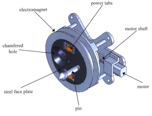
A CAD drawing of the UDP is shown in Figure 2-1. There is a pin and a hole on the

front of the UDP; when two UDPs come together to dock, the pin from one goes into 20

power tabs

electromagnet

chamfered hole

steel face plate

motor shaft

motor pin

Figure 2-1: A CAD drawing of a mostly-assembled UDP. For clarity, the drawing does

not show the wrappings of the electromagnet or the metrology boards (shown later).

the hole on the other. There is a pin capture mechanism inside each interface which captures and holds the pin from the other interface [1, 2].

Design features on the front of the UDP include:

* Electromagnet An electromagnet encircles the front plate assembly. When

two UDPs are coming together to dock, the electromagnets from each UDP attract to assist in the maneuver. The main purpose of this is to increase the docking tolerance.

" Steel Face Plate Core The core of the faceplate is made out of steel. This

increases the mass of the UDP, but the steel's mild ferromagnetic properties multiply the effect of the electromagnet.

* Power Tabs There are two spring loaded copper tabs extending from the face

plate of each UDP. By convention, the bottom one is ground and the top one

pin from second UDP

locking holes .

drive pin slot counter-rotating

locking rings

Figure 2-2: This CAD drawing isolates just the counterrotating rings of one UDP and

the pin of another. The rings have 'teardrop' shaped holes in then which, when the rings are open, allow the pin to enter, but when closed, lock the pin in place.

is power. Upon docking, the tabs from each UDP touch each other and make an electrical contact.

* Chamfered Hole and Angled Pin Head These increase docking tolerance.

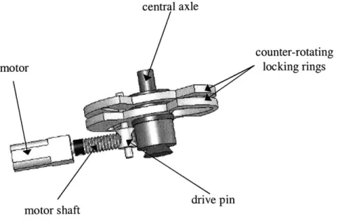
The locking mechanism in the back of the interface is shown in Figure 2-2. Two counterrotating rings allow the pin head to enter, then rotate to close around it, as detailed in the figure.

Design features of the back of the UDP include:

* Central Axle This extends through the entire interface and helps the rings

and motor shaft to be properly mounted and aligned.

* Locking Rings There are two of these rings in each interface, placed

back-to-back. Irregular shaped holes are cut in each ring such that when the rings are 'open' there is a large hole, and when the rings are 'closed' there is a small hole. The sizes of these resulting holes are designed so that the pin from another interface can enter when the rings are open, but is locked in place when the rings are closed.

rings. The slots are cut such that when the pin moves radially toward or away from the central axel, the rings open or close. The pin has a tapped hole and rides along the motor shaft.

* Motor Shaft The motor shaft is a strait threaded piece which drives the drive

pin. The shaft is connected to the motor on one end. For stability, the other

end is secured in place near the axle. The drive pin and motor shaft are shown

in Figure 2-3.

*

plate by a simple bracket.

" Pin Sensor During a docking, the UDP control board needs to know when

the pin from another interface has come far enough in for the rings to begin

closing. This is detected by an infrared optical interrupt switch. When the pin

breaks the IR beam, the UDP control board will drive the motor which will

close the rings.

" Current Spike Sensor The interface control board also needs to know when

the rings have finished rotating and have grabbed the pin, so that it can turn

off the motor. Fortunately, because of the construction of a DC motor, when

the motor hits its stop and stalls meaning the rings have finished rotating, it

will suddenly draw a large amount of current. A current spike sensor is built into the interface control board to detect these spikes and stop the motors at the correct time.

There is a circuit board (the UDP control board) which controls the functions of the interface and communicates with the module to which the UDP is attached. It controls the motor, the electromagnet, the power tabs, reads the pin sensor and the current spike sensor, receives commands from the module, and reports status to the module. There are also connections for signals from the metrology boards (discussed in Section 2.3). These signals are not processed on the interface control board, they are sent to the computer on board the module where the estimator runs.

central axle

counter-rotating motor locking rings

motor shaft drive pin

Figure 2-3: This CAD diagram shows the mechanism which counterrotates the rings. It consists of the motor, drive shaft, pin, rings, and axle.

2.3

Estimation Hardware

The interface contains the ultrasound and infrared sensors and receivers necessary for state estimation. These components are on circuit boards which are arranged annularly around the front plate assembly, as shown as a simplified CAD drawing in Figure 2-4 and as a photograph in Figure 2-5. There are three each of ultrasound receivers, ultrasound beacons, infrared LEDs, and infrared phototransistors.

When being used for estimation, it is important to know the precise locations of the ultrasound beacons and receivers relative to the CM of the module to which they are attached. These locations, of course, depend on the size and geometry of the module and the location of the UDP on the module. For each module, the estimator must 'know' the locations of the UDPs.

Figure 2-4: This CAD diagram shows the UDP with the metrology ring in place. Here, they are just modeled as green plates, but in reality, they have many electronic components mounted on them.

2.4

Conclusion

The main purpose of this chapter has been to present the design of the genderless

UDP, which is used in the projects described later in this thesis. The UDP was

de-signed under a set of requirements which included autonomy, androgyny, and netrol-ogy. The final design relies on two counter-rotating rings on each UDP to lock onto a pin from the other UDP during a (locking. The UDPs also provides the sensors used in relative state estiamtion.

ultrasound

beacon/receiver

electromagnet

V\

/ F

steel face plate

chamfered

hole

infrared receiver

power tabs

pin

infrared LED

Chapter 3

Relative Estimator

In order for two or more modules to maneuver in a collectively useful way, it is almost always necessary for the system to have knowledge of the relative or absolute positions of the individual modules. The relative position is useful in docking, tight formation flight maneuvers, or pointing operations, for example. The absolute position of the formation in the sky would be useful for applications such as ground observation, communication, or solar measurements. For most applications, the relative position must be estimated at higher frequency and accuracy than the absolute position [8, 6,

19].

This chapter is concerned with the development of a relative estimation system for multi-module separated spacecraft, specifically in the SWARM project. These modules will be performing formation control, formation reconfiguration, and docking, and all of these maneuvers require accurate measurements of the modules' relative separations and attitudes.

3.1

Architecture Choices

Depending on the other requirements of the system, the requirement of having po-sition information could be implemented in several ways. One approach is for each module to take measurements and calculate its position in an absolute global refer-ence frame (probably fixed to the Earth). Relative distances would then be calculated

by subtracting global positions. For actual formation flying satellites, however, this

is an unlikely scenario. Proximity operations often require distance measurements accurate to less than a centimeter, and it would be difficult to achieve this accuracy

by subtraction of absolute measurements, because few on-orbit satellites can measure

their absolute position around the Earth to sub-centimeter accuracy.

A better solution is to implement a relative measurement system. During most

formation flight maneuvers, especially docking, it is the relative separation which is most important. For most applications, the separation between the two modules must be known more accurately (and at a higher frequency) than the absolute position in the orbit. This is convenient because high accuracy relative measurements are easier to collect than high accuracy absolute measurements.

Another architecture choice to be made deals with where the measurements and calculations take place. For example, a single master module could take all the mea-surements, calculate the positions of each module in the formation, and communicate that position to each module. Alternatively, each module could do its own measure-ment and calculation. The hardware requiremeasure-ments for these two choices are different, and the capabilities of each differ as well.

The relative estimation system implemented here is based on the Extended Kalman Filter (EKF) technique. This chapter will describe the measurements available to the estimator and the process by which those raw measurements are reduced to filtered state estimates [131.

3.2

Available Measurements

The state sensing hardware available on each module is

" ultrasound beacons " ultrasound receivers

* infrared emitters * infrared receivers

* rate gyros

* accelerometers

The inertial sensors (gyros and accelerometers) will be considered separately. The ultrasound and infrared sensors generate separation information by measuring time of flight differences as discussed here.

During this discussion, it may be useful to keep in mind a docking operation as an example scenario. Additionally, to facilitate the discussion, the terms 'pinger' and 'detector' will be used to denote two modules involved in relative estimation. This does not have to do with a master/follower or chaser/target distinction, it is simply used to distinguish two modules for this discussion.

When it is time for a position update, one module (the detector) will emit an omnidirectional infrared pulse. The other module will detect this pulse effectively instantaneously, using its infrared receivers. At this point, the ultrasound beacons on the pinger begin emitting chirps at points in time specified by their beacon number, as shown in Figure 3-1. Beacon #1 chirps 10 ms after the reception of the IR pulse, Beacon #2 chirps 30 ms after the IR pulse, and Beacon #3 chirps 50 ms after the IR pulse. The chirps are separated by 20 ms to allow sufficient time for the energy from each chirp to dissipate. If a receiver on the detector detects a chirp 32 ms after the IR pulse, for example, then that chirp must have taken 2 ms to travel from Beacon #2. It is not possible that it took 22 ms to travel from Beacon #1, because after 20 ms the energy from Beacon #1 is fully dissipated. There is margin built into the 20 ms delay, so the estimator can confidently assume that any chirp detected came from the most recent beacon.

When all chirps and receptions are complete, each receiver on the detector has detected a chirp from each beacon on the pinger. The estimator knows when these chirps were emitted and when they were received, so using the speed of sound, the separation distance between each beacon-receiver pair can be calculated. Each of these separation distances is put into an array called the distance matrix. These nine numbers (3 receivers and 3 beacons) provide enough information to calculate the full

pinger

detector

time (Ms) t=io t=30 t=50 t=70

Figure 3-1: Timing diagram for ultrasound and infrared sensors on both modules. The dotted line at time t=O indicates the infrared flash by the detector module. The solid black lines at t=10, t=30, t=50 indicate beacon pings (the one at t=10 indicates beacon #1, and so on). The grey box on the detector's timeline from t=10 to t=20 indicates the window during which ultrasound receptions will be interpreted as coming from beacon #1 on the pinger.

relative state.

3.3

State Vector and Attitude Representation

In order to fully maneuver, the satellites need to measure their relative position, velocity, attitude, and rotation rates. The state vector is 13 elements long:

x

=

vo

where r is the position, v is the velocity, q is the attitude (represented by a quater-nion), and w is the rotation rate.

There are several ways to represent the attitude of the vehicle, such as Euler angles, a direction cosine matrix, or a quaternion. Euler angles are singular and non-intuitive. The direction cosine matrix transforms a vector in one frame to a vector in a rotated frame, but is highly redundant. The matrix has nine elements, and a general rotation only has three independent degrees of freedom, so there are six redundant parameters. The quaternion representation of attitude was chosen because it is intuitive, it is non-singular, and it contains only one redundant element. See Appendix B for a mathematical introduction to quaternions and their use in

attitude representation.

3.4

EKF Process

-

Linear Case

A brief summary of the EKF, as it applies to SWARM, is presented here. For more

detail on the Kalman filter see [17, 19]. Most of the operation of the estimator can

be presented by treating the filter as linear and the measurements as periodic; this is

done first. Following in Section 3.5, a few non-linear extensions will be presented, as

well as an extension to non-periodic measurements, to finally arrive at the actual full

relative estimator [3].

For the purposes of presenting the Kalman filter, the system model can be thought

of as a simple linear state space model with additive noise.

x

=

Ax+Bu+w

(3.2)

y

=

Cx+Du+v

where w and v are additive noise:

w

N(OQ)

(3.3)

V

~

N(O, R)

The D matrix is assumed to be zero. The noise in the system model, or process noise,

is assumed to be normally distributed with zero mean and standard deviation

Q.

Similarly, the measurement noise is assumed to be unbiased with standard deviation

R. The filter also keeps track of the estimated noise P on the state x at each time step.

The qua tities

Q,

R, and P are matricies, where each element gives the covariance

between two states or measurements. For example, the (i, i) element in P gives the

variance of the

element of the state vector, xi. The (i,

j)

element, though, gives

the co riance between xi and xj. The matrix

contains covariances at time k. The

measuroments can be considered to be taken periodically.

The EKF maintains a current best estimate of the state of the vehicle. When

a new measurement comes in at time k, the filter compares the measurements to

Xkl1 +Xk-l Xk + Xk k1 +X 1

---t

k-1

k

k+1

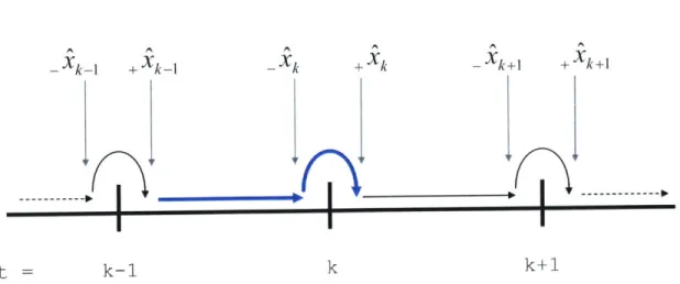
Figure 3-2: When a new piece of data comes in at time k, the estimator shown here would update the estimates using the new data, then propagate forward to the next time step (bold bllie arrows). Names of the states at each time step are shown at the top of the figure

for clarity.

the current estimated state of the vehicle and uses the two to generate a new best estimate. The filter then propagates forward to the next time a measurement is expected. This process is shown in Figure 3-2.

A note about notation - subscripts to the right of x indicate the time step, sub-scripts to the left indicate whether that state is before or after the update with '-' indicating before and '+' meaning after, and hats indicate an estimated state rather than the true state. So, for example, ik+ would indicate the estimated state at time k+ 1, but before the update. Remember that -k and +ik are both estimates at

the same time; _kk is the propagated state from the previous update without taking into account the new measurements, and +ik is an estimate of the states at the same

time, but taking into account the new measurements.

The filter takes _kk along with the measurements at time k to generate the new es-timate +ik, and the Kalman gains determine whether the propagated eses-timate (-kk)

or the actual measurement has more impact on deciding +Xk. If the measurements are more trustworthy (less noisy) than the model, then the measurements would have a larger impact on the new estimate. If the measurements are known to be very noisy, then the model propagation from the previous step would take priority. This balance is captured in the Kalman gains as described below.

data comes in at time k

previous estimates _ Xk and _P- are known

'I

compute Kalman gains

L=- PCT

(C R

Xk+1

-k+1 = A+R

PI A+ +Q

Figure 3-3: This diagram shows the basic cycle of the linear Kalman filter. It begins at the top with new data coming in.

Once a new piece of data becomes available, the EKF follows the following general cycle, described in this section and illustrated in Figure 3-3 [18].

1. compute Kalman gains

2. update state estimates

3. update covariance

4. propagate

When a new measurement comes in at time k, the propagated estimates from the previous update, -xk and -Pk are known. Now, Kalman gains Lk must be computed.

Lk= _PC(CPCT

₊

33

update stat estimate

This takes into account the covariance of the previous estimates -Pk and the

noise in the sensors R to create a set of gains which will control how much the new measurements are able to alter the new state estimate. The new state estimate +±k

is then calculated using the Kalman gains according to

+Xk = -Xk + Lk(yk - C-ik) (3.5)

We have the new updated state estimate +kk, and we must also update the covariance matrix P. The covariance matrix is updated using

+Pk = (I - LkC) -Pk (3.6)

Now, the update phase (the 'hop' at time k in Figure 3-2) is complete, and the only remaining task is to propagate in preparation for the next measurement at k +1. With this system model, the state propagation is simple:

-Xk+1 = Ad+ik (3.7)

where the subscript d emphasizes that Ad is part of a discretized, not continuous, system model. At this stage, the control inputs are not accounted for in the prop-agation, see Section 5.1.4 for a discussion of this as future work. Propagating the covariance matrix is simple as well, keeping in mind that the model noise Qk must be included.

-Pk+1 = Ad +Pk Ad

+

We now have XIk±1 and -Pk+1, which when the filter runs the next time will

become ikk and -Pk, so the filter is complete and ready to be run again.

3.5

Nonlinearities

Two extensions to the linear periodic Kalman filter have been made for the relative estimator. The first allows for non-periodic measurements, and the second allows for

Xk-1 + Xk-1 -k + Xk -k+1 + Xk+1

t

k-1

k

k+1

Figure 3-4: When a new piece of data comes in, the estimator shown here would first propagate the state from the last known time to the clurrent time, then update the estimate with the new data (bold blue arrows).

non-linear system model and non-linear measurements. They will be presented in this order.

3.5.1

Nonperiodic Measurements

The real system has both ultrasound measurements and gyro measurements. These two forms of data do not come at the same frequency, and occasionally, an ultrasound receiver will 'drop out' for one cycle. This means that it is not possible to predict when the next measurement will occur. The filter must be able to handle this.

The consequence for the filter presented above is that it is no longer possible to propagate at the end of the cycle. The last step is to take +kk and propagate it forward in time to the point of the next measurement, creating Xk+, but this is no

longer possible because the filter would not know when the next measurement will be available so it would not know how far forward to propagate.

The problem can be solved by simply changing the order of steps in the filter. When the filter begins, it will be given +kk-1 and its first step will be to propagate to the present time. It will then compute gains and update the measurements. In effect, the diagram has been changed to the one shown in Figure 3-4.

a O

66

00b

1

2

3 4

Figure 3-5:

Crosses represent beacons and circles represent receivers. If a receiver is at

position 1 and moves slightly to position 2, then the measurement (distance between beacon

and receiver) will change by a small amount. However, if the receiver is at position 3 and

moves slightly to position 4, then the measurement will change by a larger amount. This

is evidence of nonlinearity in the relationship between change in measurements and change

in states.

3.5.2

Nonlinear Measurements

The ultrasound measurements from the UDPs are definitely nonlinear. Consider the

case of two UDPs facing each other. If one UDP moves slightly, the ultrasound

distance measurements will change by a certain amount, as shown in Figure 3-5.

However, if the UDPs are separated transversely and move by the same amount, then

the measurements will change by a different amount.

The use of the C matrix above implicitly ignored this problem, now we must

correct it. The correction can be made by creating a full nonlinear model of the

sensor behavior, and linearizing a C matrix at each time step. The linearized C is

the Jacobian, called H.

The plan is to find the function

which outputs the expected

measure-ments given the state of the system, then differentiate that function. The function

hk(x(tk))

is a vector valued function of a vector, so its derivative will be a matrix,

the Jacobian H. The linearized C matrix at each time step is the Jacobian at that

time step,

H

=

(3.9)

&X(tk) X(tk)=-k

Chaser

Target

X

Figure 3-6: This figure shows the notation of the position of beacons and receivers in the reference frames of the two modules. Crosses represent beacons and circles represent receivers. The beacons and receivers would actually be on a UDP, of course, but for clarity, just the SPHERES satellite and the beacons and receivers are drawn.

that one module has beacons pinging, and the other module uses its receivers to measure the pings. The module with beacons pinging will be called the target and the module with receivers active will be called the chaser. As before, this has nothing to do, in principle, with a target/chaser distinction in a docking maneuver, they are just names to distinguish the two. The filter must 'know' the locations of the beacons and receivers relative to the CM of each module, but reference frames are important to specify. As shown in Figure 3-6, the position of beacon number i in the body coordinates of the target module will be denoted bfT. The position of receiver number

j

j

The first step is to calculate the expected measurements h given the state of the vehicle x. This calculation, like most in this section, will take place in the reference frame of the target (the module with active beacons). The measurements are times

of flight of ultrasound signals, which are converted into distances using the speed of sound. So, for each beacon ping, h is a vector containing separations between a beacon and each receiver. In other words, when beacon i pings, the jth element of h is the separation distance between beacon i on the target and receiver j on the chaser. Calculating their separation distance is simply a matter of finding all their positions in one reference frame and subtracting.

The mechanical construction of the modules and the UDP dictates bTT and s7c

These are hard coded in the software. The quantity that changes is s'7. Finding s7T knowing the relative state of the two vehicles is simple:

sCT

= QsCC +

(3.10)

where

Q

j

to beacon i is

di = - T (3.11)

but the ultrasound metrology system only measures the magnitude of the separation, not the full vector, so the distance from the beacon to receiver

j

hj = djj (3.12)

= T - SCT 2 + (bTT - SCT) 2 + (bT - SCT) 2 (3.13)

This is the function hk(Xk). The elements of the state vector Xk do not explicitly appear in Equation 3.13, but they are involved in calculating sCT in Equation 3.11. The position appears as r, and the attitude quaternion is required in calculating the rotation matrix

Q.

Now, we must find the Jacobian, H, which is 9. The number of rows of H will be the number of measurements (number of receivers), and the number of columns will be the length of the state vector.

state length (13)

E

It can be seen at this point that H will only have 7 non-zero columns, the other

6 columns will be full of zeros. Only 7 of the state elements appear in

-

the

position and attitude states. The velocity and rotation rate state elements do not

appear at all, so their derivatives will be zero.

Block #1 describes how changing each position state element affects each

mea-surement, and Block #2 shows how changing each attitude state element affects each

measurement.

To calculate Block

#1,

(b.T

+

(b'T

a

(bTT

₊

Or

Or

1 1

-!2 (b

(b

(bTT

1

S3)

-(3.17)

To analyze the vector derivative, consider it one element at a time. For the rx component,

Ohi bT - sCT

O

9r~

+

)

for the ry component,

b TT - sqT

b T

+ (bST

+ bi-

sT )

and for the r, component,

So,

0h

Or

Oh

Or

This completes the calculation of Block #1.

For Block #2, we must differentiate the measurements hi with respect to the attitude of the module, contained in the rotation matrix

Q.

ahq

₁

_(bTT

Oq

\

oq

i S

The vector derivative ' can be broken down by splitting it into three general com-ponents (u,v,w). Recall that b.T - can be written as dij, as is done for Equation

3.24.

Ohi

(

=

d

q

(d)

OU

+

O(di)

_{+ a (d j)}

09

Ow)

(3.24)

If the vector (u,v,w) is set equal to QsjC, then Equation 3.24 reduces to

bTT

(O

X

+

QsC)

(3.25)

+

QsC)

(3.19)

(3.22)

bzx

bTT

h4

Ohi

+

sy

+

z

j

However, s7T is a constant, so it can be removed from the derivatives.

Oh_

bTT

-

s T

(Q

cc

q = - - s 3 (3 .2 7 ) Now, we must calculate '. To generate a rotation matrix from the elements of a quaternion, the relationship is [13]:

F2

(l2+~4

q-

q2-

Q(q) = 2(q1q2- qq4) -q2 +q2 - q2 + q2 2(q2q3+ qq4) (3.28)

2(qiq3 + q2q4) 2(q2q3 qlq4)

-q

-

Differentiating all nine of these elements by each of the elements of q creates a quantity with three dimensions and 36 elements. Each differentiation is simple, so they will not be explicitly shown here. They are contained in a piece of code attached in Appendix A.4.

We can now construct H, using Equation 3.22 for Block #1, and Equation 3.27 for Block #2. This completes the development of nonlinear measurement capability in the relative estimator.

3.6

Prefilter

As will be discussed and analyzed in Section 4.1, the ultrasound sensors sometimes give bad readings. They occasionally give a reading which is obviously incorrect (a meter off, for example), and they sometimes miss readings all together and return zero. In either of these cases, this erroneous data could throw off the estimator. It is helpful to have a prefilter before the estimator to screen the data. The prefilter currently has three stages.

* Remove Zeros When a receiver returns exactly zero for its measurement, it

means that the receiver did not receive anything. It doesn't actually mean that the beacon and the receiver are very close, it just indicates a missed reading.

These cases are removed by the prefilter, so the data does not get to the esti-mator where it would be interpreted as the beacon and receiver being separated

by 0 cm.

* Remove Geometrically Impossible Readings The receivers on the UDP

are separated by fixed distances. If two receivers give readings that are off by more than the largest of these distances, than one (or both) of the readings is wrong. Instead of figuring out which one is correct (which takes time and is not always possible), the prefilter throws out the whole update, and the estimator just propagates through that time step without a measurement update.

" Remove Large Readings The ultrasound energy from a beacon dissipates

after 3 meters, so any readings larger than that must be incorrect. They are removed.

3.7

Conclusion

This chapter presented the core theoretical basis for the EKF-based relative state estimator. Data for the estimator comes from the ultrasound range measurements between beacons and receivers. To generate a new state estimate each time new data becomes available, the estimator follows a four step process - propagate, com-pute Kalman gains, update state estimate, and update covariance. For actual imple-mentation, there are several nonlinear extensions to the basic linear Kalman filter, including the nonlinear measurement model and the ability to handle nonperiodic measurements. To further filter the data, a prefilter runs before the estimator to screen out obviously erroneous measurements. The next chapter will cover actual testing of the estimator.

Chapter 4

Results and Applications

This chapter discusses the use of the relative estimator in several relevant hardware

projects. The estimator is most useful and enabling in projects involving

modular-ity, formation flight, docking, and reconfiguration. The projects discussed here are

SWARM (Synchronized Wireless Autonomous Reconfigurable Modules) and SIFFT

(Synthetic Imaging Formation Flight Testbed).

The relative estimator was tested in three phases. First, a low-level verification

and analysis of the ultrasound receivers was carried out. This test was necessary to

show that the receivers gave steady and accurate time-of-flight measurements, and

that they did not respond to extraneous ultrasound energy. Second, the full estimator

was coded in Matlab@ and then run on actual data. This showed that the estimator

was coded correctly and that the estimates produced were reasonable. Third, the

estimator was translated into

C

code and run in actual docking experiments on real

hardware. This is the final test of usefulness for the estimator. Each of these three

phases of testing is described in this chapter.

4.1

Testing of Ultrasound Receivers

To test the ultrasound receivers (and beacons), a beacon-receiver pair was placed a

fixed distance apart, and a large number of time-of-flight measurements was taken.

The measurement here is just the pure time delay of the ultrasound ping, there is

30- 25-E 20-E 15-C,) E 10-

5-0

time (s)

Figure 4-1: This plot shows 60 seconds of data for one beacon-receiver pair. Overall, the data is very consistent. Notice one error at approximately 10 seconds, and several zero readings, indicating times when the sensor temporarily dropped out.

no filtering or estimation. Because neither the beacon nor the receiver is moving, the expected result of the test is that all the measurements will be tightly clustered around the actual separation. The most useful result of this test, though, will be to determine if the receivers commonly pick up ultrasound noise produced in the environment, if they commonly detect pings from the previous beacon (echoes), or if they commonly miss a ping altogether.

Because there are three receivers and three beacons on each UDP, many combi-nations of beacon-receiver pairs were tested. If just one beacon and one receiver were chosen for this test, then the results would not be generalizable to all pairs.

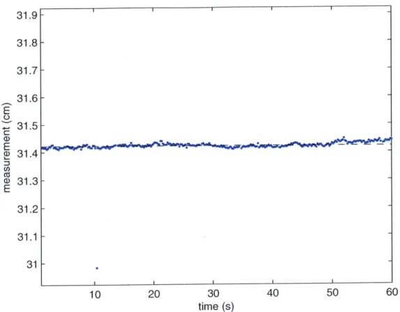
Figure 4-1 shows the time series data from a single beacon-receiver pair. The beacon is pinging at 5 Hz for 60 seconds. Clearly, the measurements are very steady

31.9- 31.8- 31.7- 31.6-E U 31.5-E Co) a) 31.3-E 31.2 31.1 31 -10 20 30 40 50 60

time (s)

Figure 4-2: This plot shows the same data as Figure 4-1, but zoomed in so that the entire vertical axis represents 1 cm. Except for one outlier, all the data falls within about half a millimeter.

with no large scale deviations. There are occasional large errors and occasional zeros. In this data set, there are six zero measurements, when for unknown reasons, the sensor did not read anything (so returns zero). There is one case (just after 10 seconds) where the sensor did record a different, non-zero range, but the reading was wrong. Overall, in this data set, 2% of the measurements were missed (zero), and

less than 1% were non-zero but erroneous.

Figure 4-1 does not show the small amount of noise around the mean. In Figure 4-2, the vertical axis is tightened to half a centimeter on either side of the mean to show this behavior. Even at this small scale, the sensor is still quite consistent - the standard deviation of the measurements is only 0.267 nn.

A missed mieasuremiemit is not really a reading of zero, it is just a time when no

---Table 4.1: Summary of results from single beacon-receiver pair test.

number of measurements

300

standard deviation (mm)

0.267

number of lost measurements

6

percentage lost

2%

data came in. The prefilter will remove these data points before they even get to the

estimator. Table 4.1 sumarises the data from this test.

The data also shows that the sensor does not often receive signals from extraneous

ultrasound sources and record them as data. This is significant because it is possible

that there could be such sources in the environment in the lab (or in the space station),

but they do not seem to cause frequent errors in the data.

This data is just from one beacon-receiver pair in a time series. Although it is

useful to analyze the data like this to make sure that there are no large scale or low

frequency errors, it is more useful to analyze all data from all beacon-receiver pairs

and analyze their deviations from their expected values. To this end, a larger set of

data was collected (in several runs). In each run, data was collected from all nine

possible beacon-receiver pairs. That's approximately 60 seconds of data from each

pair. A total of seven data runs were carried out for a total of 16947 measurements.

So, for a given beacon-receiver pair, approximately 60 seconds of data was taken and

this was repeated seven times.

Let Tij, represent the set of measurements taken from receiver

j

of the distance

to beacon i during run

r.

(The data plotted in Figure 4-1 and Figure 4-2 happens to

be T

.) With data being taken at 5 Hz for approximately 60 seconds, each Tij, will

contain approximately 300 measurements. To compare data from one beacon-receiver

pair to another, the means are subtracted out and just the errors are analyzed.

Tijr ( Tijr - An(Thjr)

(4.1)