A decomposed symbolic approach to reactive planning

(1)

A DECOMPOSED SYMBOLIC APPROACH TO

REACTIVE PLANNING

by

Seung H. Chung

B.A.Sc., Aeronautical and Astronautical Engineering University of Washington, 1999

SUBMITTED TO THE DEPARTMENT OF AERONAUTICS AND ASTRONAUTICS IN PARTIAL FULFILLMENT OF THE REQUIREMENT FOR THE DEGREE OF

MASTER OF SCIENCE at the

MASSACHUSETTS INSTITUTE OF TECHNOLOGY

June 2003

@

MASSACHUSETTS INSTITUTE OF TECHNOLOGY

SEP 1 0 2003

LIBRARIES

Signature of Author ...

Department of Aeroautics and Astronautics May 23, 2003

Certified by ... ...-- -- ...

Brian C. Williams

Associate Professor of Aeronautics and Astronautics Thesis Supervisor

Accepted by ... . ---- -. . . .

--Edward M. Greitzer

H.N. Slater Professor of Aeronautics and Astronautics

Chair, Department Committee on Graduate Students

(2)

(3)

A Decomposed Symbolic Approach to

Reactive Planning

by

Seung H. Chung

Submitted to the Department of Aeronautics and Astronautics on May 23, 2003, in partial fulfillment of the

requirements for the degree of Master of Science at the Massachusetts Institute of Technology

Abstract

Autonomous systems that operate in uncertain dynamic environments must respond to unanticipated events and goals by reconfiguring themselves in real-time. Reactive plan-ning achieves reconfiguration in real-time by constructing a goal-directed plan (GDP) for

all possible events and goals offline and then executing the GDP online, while monitoring the outcome of each execution step. A GDP, however, is susceptible to an explosion in space that is proportional to the square of the system's state space.

This thesis presents a new reactive plan encoding called a decomposed goal-directed plan (DGDP), which addresses the state space explosion problem by unifying two

com-plementary approaches in the literature: transition-based decomposition and symbolic encoding. The DGDP encoding first uses transition-based decomposition to reduce the overall complexity of the planning problem by dividing the problem into a set of subprob-lems that may be solved independently, and then combined serially. This decomposition is based on the structure of the system's transition dependency graph (TDG), which cap-tures the transition dependencies among the system components. Next, a GDP for each subproblem is generated using a compact symbolic encoding in terms of Ordered Bi-nary Decision Diagrams (OBDD). Finally, these GDPs are combined into a full plan, the

DGDP, based on the transition-based decomposition. This thesis makes two additional

contributions to state-of-the-art reactive planning. First, it generalizes the "divide-and-conquer" approach introduced by the Burton reactive planner to systems with interde-pendent components, where a system with interdeinterde-pendent components is characterized

by cycles within its TDG. Second, it generalizes OBDD plan encodings from universal

plans, which are conditioned on all possible initial states, to goal-directed plans that are also conditioned on all possible goal states. The new decomposed symbolic reactive planner is empirically validated on representative spacecraft subsystem models.

Thesis Supervisor: Brian C. Williams

Title: Associate Professor of Aeronautics and Astronautics

(4)

(5)

Acknowledgments

This thesis is dedicated to my parents, Shin-Kwan and Young-Soon Chung. They are the source of all knowledge I deem most invaluable. They taught me of faith and love. They will remain the greatest teachers of my life, and I will eternally be grateful to them. I also thank my sisters, Hee-Won Chung and Hee-Sun Chung, for their love and friendship.

I especially thank my advisor, Professor Brian C. Williams, for his inspirational

breadth of knowledge and guidance through which this thesis was made possible.

I thank Michel Ingham for his support and encouragement, not to mention his

leader-ship as the senior graduate student of the Model-based Embedded and Robotic Systems Group. I also thank Paul Elliott and Robert Ragno for the discussions on C++ coding styles, and the rest of the Model-based Embedded and Robotic Systems Group members who worked together as a team in the development of the model-based executive.

A special thanks goes to Margaret Yoon, Greg Sullivan, and Mark Hilstad for their

time commitment in proof-reading this thesis. I thank David Watson and Mike Pekala at the Johns Hopkins University Applied Physics Laboratory for being supportive of the model-based technology research and development. I thank all MIT students in the Space Systems Laboratory who have provided great moral support.

Most importantly, I thank God for His grace and blessings.

This research was supported in part by NASA's Cross Enterprise Technology Develop-ment program under contract NAG2-1466, DARPA's MOBIES program under contract

F33615-OOC-1702, and NASA Graduate Student Research Program Fellowship.

(6)

(7)

List of Figures

1-1 Model-base Executive. . . . . 17

1-2 Mode Reconfiguration . . . . 18

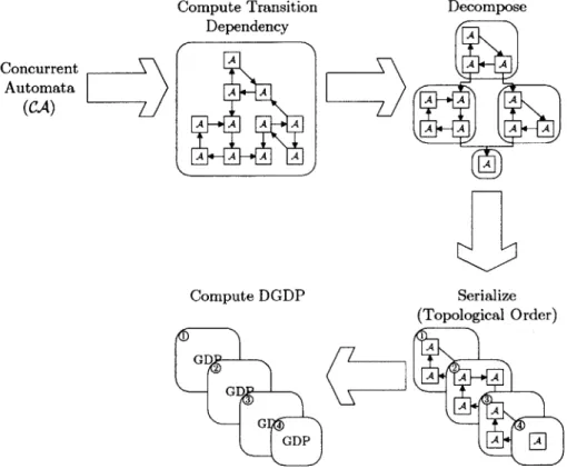
1-3 Decomposed Goal-directed Planning Process . . . . 22

2-1 MESSENGER Telecommunication System . . . . 27

2-2 MESSENGER Antenna Locations . . . . 29

2-3 Simplified Telecommunication System . . . . 31

2-4 Bus Controller Model . . . . 32

2-5 Transmitter Model . . . . 32

2-6 Amplifier Model . . . . 34

2-7 Antenna Model . . . . 35

3-1 Amplifier Automaton . . . . 41

3-2 Bus Controller and Transmitter CA . . . . 43

3-3 OBDD Examples . . . . 46

3-4 Amplifier States and State Space OBDDs . . . . 47

3-5 Amplifier Automaton without Fault Transitions . . . . 48

3-6 Transition and Transition Relation OBDDs . . . . 50

4-1 Composed Automaton of a System . . . . 54

4-2 Transition Relation Size vs. Number of States . . . . 57

4-3 Goal-directed Plan . . . . 58

5-1 Bus Controller and Switch Concurrent Automata . . . . 67

5-2 Transition Dependency Graph . . . . 69

5-3 SCC Composed Automaton . . . . 70 11

(12)

5-4 T1/A1 SCC Composed Automaton GDP . ...

6-1 Bus Controller SCC Composed Automaton GDP

6-2 T1/A1 SCC Composed Automaton GDP . ...

6-3 Simplified Telecommunication System TDG . .

6-4 Three Types of TDGs ...

7-1 GDP and DGDP Size vs. Number of States . .

(x1 4 X2)A (X3 4 x 4) OBDD ...

Three BDD Reduction Methods ... BDD Reduction Example ...

Reduced Ordered Binary Decision Diagram. Restrict Operation ... . . . . 99 . . . . 100 . . . . 101 . . . . 101 . . . . 102 71 78 78 79 85 92 A-1 A-2 A-3 A-4 A-5

(13)

List of Tables

3.1 Amplifier Transition Function . . . . 7.1 BuDDy Functions for OBDD Operators.

7.2 Plan Size Comparison . . . .

A.1 BDD Operation Time Complexity . . . .

13

. . . . 4 1

. . . . 88 . . . . 9 1 . . . . 104

(14)

(15)

Chapter 1 Introduction

NASA's MErcury Surface, Space ENvironment, GEochemistry, and Ranging (MESSEN-GER) mission will launch in March 2004 to explore Mercury for the first time in nearly

30 years. One of the most critical stages of the mission is Mercury orbit insertion (MOI). A fault during this stage could cause the MESSENGER spacecraft to either crash into

Mercury or miss Mercury altogether, resulting in mission failure.

Traditionally, a ground operator controls a spacecraft by uploading the necessary sequence of commands. However, this type of open-loop commanding lacks robustness. Especially, if an anomaly occurs during the execution of the command sequence, the spacecraft could not only fail to achieve the intended objective, but the execution of the remaining commands in the sequence, given an off-nominal state, could potentially have disastrous effects.

If a spacecraft and its operational environment always behaved exactly as expected, open-loop commanding would suffice. Due to possible occurrences of anomalies, however, closed-loop control is necessary. Typically, control is provided with ground operators in the loop. While ground operators are very capable, their ability to react to anomalies is limited by the communication-time delay. For example, MESSENGER and Earth are so distant during MOI (approximately 200 million kilometers), that round-trip commu-nication is delayed by approximately 21 minutes. If an unanticipated fault arises within 21 minutes prior to MOI, the spacecraft will be helpless.

Missions, like MESSENGER [1], use onboard rule-based systems for fault recovery. Rule-based system reactions are not limited by communication delay, but their recovery capability is limited to only the set of faults predicted by the engineers. Also, as spacecraft

(16)

become more complex to accommodate ambitious mission requirements, hand coding robust recovery rules becomes more arduous and prone to error. Thus, a new type of onboard reactive system is necessary to autonomously respond to anomalies.

1.1 Model-based Executive

Remote Agent, which flew on board Deep Space One (DS1) as one of the New Millennium Program technologies, provided the first demonstration of fully autonomous and adaptive operation of a spacecraft [27, 26]. Embracing the essential features of Remote Agent, the concepts of model-based programming and execution were developed to address the problems in traditional software development practice that can lead to software that is unreliable and lacks modularity and portability [30, 29]. Model-based programming was developed as an instance of the "executable specification" paradigm, in which a specification is automatically translated into system interactions by the model-based executive. This is in contrast to the traditional approach of hand translating a software implementation into a specification used for verification, where the hand coding opens up a considerable potential for human introduced errors. Model-based programming is distinguished from other executable specification languages [20, 4] in that it is state

and fault aware. Specifications are expressed at a high level in terms of hidden state evolutions, rather than through detailed command and observation sequences. This allows the error prone process of reasoning through system interactions to be delegated to the model-based executive. Specifications are fault aware, in that they include models of the physical plant's nominal and faulty behaviors. This allows the executive to act appropriately during failure in order to achieve the specified state evolutions.

A model-based executive consists of two components, a control sequencer and a

de-ductive controller, as shown in Figure 1-1 [29]. The control sequencer is responsible for generating a sequence of configuration goals using the control program and the plant state estimates. Each configuration goal specifies an abstract state of the plant to be achieved.

(17)

1.2 Motivation for Tractable Reactive Planning

Figure 1-1: Model-based executive architecture.

(ME) and Mode Reconfiguration (MR) (see Figure 1-1). The two software modules along with the physical plant (e.g., spacecraft hardware) form a closed-loop control system. The ME module estimates the most likely state of the plant that is consistent with the model, the observations from the plant sensors, and the knowledge of the executed commands. Given the state estimates from ME, the MR module generates the commands necessary to achieve the goals specified by the control sequencer. Fault protection is inherent to this closed-loop architecture. In the event of a fault, ME diagnoses the faulty state, and MR immediately attempts to command the plant out of the faulty state and into the goal state that corresponds to the configuration goals. If such a command exists, MR executes it, thus recovering from the fault.

The MR module is comprised of two submodules as depicted in Figure 1-2. The first submodule is Goal Interpretation (GI). GI takes the configuration goals and generates the goal state that satisfies the configuration goals. The second submodule is the Reactive Planner (RP). RP determines and executes the command that will progress the plant from the estimated state to the goal state. The focus of this thesis is the RP submodule.

1.2 Motivation for Tractable Reactive Planning

While any general-purpose onboard planners could be put in place of the reactive planner, due to the PSPACE-complete nature of planning problems [9], real-time response cannot

(18)

Configuration Goal

Estimated State Command

Figure 1-2: Mode Reconfiguration submodule of the deductive controller.

be guaranteed by a general-purpose planner. In time-critical situations, such as MOI, late response to a fault could be disastrous for the mission. A reactive planner compiles a plan offline for all possible situations, and then executes the plan online. Reactive planning is an approach that guarantees real-time response.

One of the early approaches to reactive planning is universal planning [28]. Given a goal state, a universal plan maps a set of all possible initial states to the actions that lead towards the goal state. With a universal plan, the correct sequence of actions can be decided at the execution-time, while observing the outcome of each action. Although universal plans provide the means to react to a nondeterministic environment in realtime, Ginsberg pointed out the intractability of universal planning due to the exponential state space explosion problem [18].

In addition, a universal plan cannot react to rapidly changing goals. Since a universal plan is valid only for a specific goal, a new universal plan must be generated for each new goal. As such, realtime response cannot be guaranteed when the goal changes. For example, if the primary propulsion system of MESSENGER fails just prior to MOI, the secondary propulsion system must be turned on, that is, a new goal state must be achieved.

Alternatively, Burton reactive planner produces a goal-directed plan (GDP) that can react to all possible initial states and goals as well. Burton is innovative for its use of a "divide-and-conquer" approach that divides a planning problem into smaller subprob-lems. This permits Burton to encode an extremely compact plan, where the plan's size

(19)

1.3 Thesis Contributions 19

is linear in the number of system components. However, Burton's reactive planning ca-pability is limited to problems in which no components are interdependent, that is, no two components may depend on one another for their transitions.

1.3 Thesis Contributions

This thesis presents a new reactive plan encoding called a decomposed goal-directed plan

(DGDP), which addresses the state space explosion problem by unifying two

complemen-tary approaches in the literature: transition-based decomposition and symbolic encoding. The DGDP encoding first uses transition-based decomposition to reduce the overall com-plexity of the planning problem by dividing the problem into a set of subproblems that can be solved independently, and then combined serially. Next, a GDP for each subprob-lem is generated using a compact symbolic encoding in terms of Ordered Binary Decision Diagrams (OBDD). Finally, these GDPs are combined into a full plan, the DGDP, based on the transition-based decomposition.

This thesis makes two additional contributions to state-of-the-art reactive planning. First, it generalizes the "divide-and-conquer" approach introduced by the Burton reactive planner to systems with interdependent components. Second, it generalizes OBDD plan encodings from universal plans, which are conditioned on all possible initial states, to goal-directed plans that are also conditioned on all possible goal states.

1.3.1 Handling State Explosion through Decomposition

The method of divide-and-conquer is a well known, effective approach to solving prob-lems. The transition-based decomposition approach [31] leveraged in this thesis is an approach that effectively divides a planning problem into subproblems. This decomposi-tion is based on the structure of the transidecomposi-tion dependency graph (TDG), which captures the transition dependencies among the system components. Although this method is very different in its specifics from that of the structural decomposition methods used for constraint satisfaction (CSP), database theory, and Bayesian Network problems, the con-tribution of transition-based decomposition to planning is analogous to that of structural

(20)

decomposition methods.

CSPs are known to be NP-complete in general; however, Freuder has shown that a

CSP with a tree-structured constraint graph is solvable in linear time [17]. Similarly,

Williams and Nayak have shown that if a planning problem has an acyclic TDG (i.e., the dependency among all components with respect to the transition conditions is unidirec-tional), then the problem can be solved within a state space that grows linearly in the number of system components [31]. For CSPs that do not have a tree-structured con-straint graph, Dechter and Pearl have shown that the concon-straint graphs of those problems can be transformed into tree-structured graphs using a tree decomposition technique [16]. For planning problems with cyclic TDG (i.e., some components are interdependent), this thesis introduces a transition-based decomposition that transforms a cyclic TDG into an acyclic TDG. Thus, through the transition-based decomposition technique, even planning problems with cyclic TDG can be solved within a state space that grows approximately linearly in the number of system components.

1.3.2 Handling State Explosion through Symbolic

Representa-tion

The transition-based decomposition method reformulates a problem into a set of subprob-lems, then the global solution is constructed from serial solutions to the subproblems. The transition-based decomposition method addresses the state space explosion prob-lem at the global level, similar to Burton, but then uses symbolic encoding methods to address the explosion problem difficulty at the subproblem level.

The logic synthesis and model checking communities have made very effective use of a symbolic representation called Ordered Binary Decision Diagrams (OBDD) [6] to con-struct compact state space encodings. An OBDD-based model checking technique has proven particularly successful in dealing with the state space explosion problem [8]. Rec-ognizing the similarities between model checking and planning, Cimatti et al. introduced a new universal planning technique that takes advantage of the OBDDs [11]. Since then, several OBDD-based universal planning algorithms have been developed for operating

(21)

1.4 Thesis Outline 21

within nondeterministic domains [13, 12, 21]. Likewise, the new reactive planning ap-proach adopts the OBDD encoding technique to compile the goal-directed plans (GDP) that can react to the nondeterministic environment as well as rapidly changing goals. In essence, a GDP maps all possible situations and goals to an action that is guaranteed to progress the system toward the goal state. The GDPs of the subproblems are combined into a decomposed goal-directed plan (DGDP) for the entire planning problem.

1.4 Thesis Outline

The remaining chapters discuss a new approach to reactive planning that unifies the aforementioned decomposition and symbolic representation methods. Figure 1-3 outlines the planning process that computes DGDPs:

First: A behavioral model of a system is represented as concurrent automata, CA. In addition, for compactness these concurrent automata are encoded in OBDDs.

Second: The TDG of the concurrent automata is computed. The TDG describes how the transitions of an automaton depend on other concurrent automata.

Third: A cyclic TDG is transformed into an acyclic TDG by decomposing the system

into smaller subsets. Then, the concurrent automata in each subset are composed into a single automaton.

Fourth: The composed automata are serialized in topological order.

Fifth: A DGDP is produced by computing a GDP for each composed automaton in

topological order.

To set the context of this technical development, a spacecraft telecommunication sys-tem example is first introduced in Chapter 2. This example is used to help guide the reader throughout the aforementioned planning process. Chapter 3 maps to the first planning process. This chapter defines a concurrent automata formally and presents an

(22)

Compute Transition Dependency Concurrent Automata (CA) Compute DGDP Decompose A A A A A A A A A A A Serialize (Topological Order)

Figure 1-3: Decomposed goal-directed planning process.

E*

(23)

1.4 Thesis Outline 23

OBDD representation of the concurrent automata. Before going into the details of de-composition, Chapter 4 introduces the method for computing and executing a GDP using a symbolic encoding. The algorithms outlined in this chapter also provides the founda-tion for computing DGDPs. Chapter 5 then discusses the decomposifounda-tion, serializafounda-tion, and DGDP computation. This chapter's discussions correspond to steps 3 through 5 of the planning process mentioned above. Chapter 6 discusses how a DGDP is executed, followed by Chapter 7, which provides a discussion of implementation and experimental results. Finally, Chapter 8 provides concluding statements and future work.

(24)

(25)

Chapter 2 Spacecraft Telecommunication

System

NASA's MErcury Surface, Space ENvironment, GEochemistry, and Ranging (MESSEN-GER) mission will launch in March 2004 to explore Mercury for the first time in nearly

30 years. The objective of the mission is to further our understanding of Mercury's

geological and atmospheric characteristics, ultimately advancing our knowledge of the terrestrial planets and their evolution. The telecommunication system is one of the spacecraft's critical subsystems required to achieve MESSENGER's objective. Without the telecommunication system, the commands necessary to carry out the science activ-ities cannot be uploaded to MESSENGER and science data cannot be downloaded to Earth; without the science data, the mission will be a failure.

Maintaining an operational telecommunication system is crucial for the mission. If a reparable fault occurs in some component of the telecommunication system, it must be restored to an operational state immediately. An offline telecommunication system would result in the loss of science opportunities, as no commands can be uploaded to initiate any science activities. In the worst case, ground operators will be incapable of uploading the commands that initiate time-critical maneuvers, such as orbit insertion around Mercury, resulting in complete mission failure. Furthermore, since the ground operators cannot upload the commands necessary to repair the faulty telecommunication system, this repair operation must be autonomous.

As such, the telecommunication system is an appropriate example for illustrating an autonomous repair capability based on reactive planning. Furthermore, the complexity

(26)

and redundancy that the telecommunication system possesses presents an ideal scenario for an autonomous reconfiguration demonstration. This chapter introduces MESSEN-GER's telecommunication system design and provides a functional description of its components. Finally, a simplified, yet representative telecommunication system is in-troduced. The remaining chapters will use the simplified telecommunication system to describe the decomposed symbolic approach to reactive planning.

2.1 MESSENGER Telecommunication System

Due to its criticality to the mission, MESSENGER's telecommunication system was designed to be fully redundant with no credible single-point failures. As illustrated in Figure 2-1, the telecommunication system consists of two X-band Small Deep Space Transponders (DST), a hybrid coupler, two solid-state power amplifiers (SSPA), two radio-frequency (RF) switch assemblies, and eight antennas. A computer and a 1553 bus controller, a simplified integrated electronics module (IEM), were added to complete the data flow. In this section, each of these components is described in more detail.

Integrated Electronics Module

The IEM consists of three components: a computer, a 1553 bus controller, and a 1553 bus. The IEM's computer generates all data to be transmitted to Earth, and all data received from Earth is routed to the computer. The computer also commands all controllable devices (e.g., commanding the transponder to be on or off). The 1553 bus controller is responsible for directing the flow of data and commands between all devices connected on the 1553 bus. For example, the bus controller directs data to be downloaded to the appropriate DST, and routes the data received in the latest uplink by a DST back to the computer. Though the MESSENGER design includes a redundant IEM, only one is shown for the clarity of the diagram.

(27)

2.1 MESSENGER Telecommunication System 27

IEM Telecommunication System

Small DST#1 RF Switch Assembly #1 LGA (-Y)

3-

- Receiver

LGA (-Z)

- - Transmitter, - - SSPA #1 -+Diplexerean(Y

Fanbeam (-Y)

Phased _(Y

1553 Aay #1Swirih

Computer -Bus -ouHybr

Controller _CuerPhased (Y Array #2 Fanbeamn (+Y) Trnmttr- _{+SSPA #2} _Diplexer LA(Y

X-Band RIF Switch Assembly #2 1 LGA (+Z)

Small"DST #2

Figure 2-1: On the right side of the dotted line is the schematic of the MESSENGER telecommunication system [1]. To the left of the dotted line is a simplified schematic of MESSENGER's integrated electronics module (IEM).

(28)

Deep Space Transponder

Two DSTs are available within MESSENGER for redundancy. Each DST consists of a transmitter and a receiver. The transmitter converts the downlink data to an X-band signal that is appropriate for transmission via available antennas. The receiver converts the received X-band uplink signal into data that is recognizable by the computer.

Hybrid Coupler

A hybrid coupler is a passive device that distributes the signal from each transmitter to

two SSPAs. The design of the hybrid coupler is very simple; as such, its failure rate is low enough not to be considered a credible point of failure, and no redundancy is necessary.

Solid-State Power Amplifier

Two SSPAs are available for redundancy; each one is associated with one RF switch assembly. Each SSPA is capable of amplifying the signal strength to the level required for transmission via one of the available antennas.

RF Switch Assembly

The amplified signal from each SSPA is sent to the corresponding RF switch assembly. An RF switch assembly is comprised of a diplexer and a series of switches. A diplexer allows the antennas to be used for both transmitting and receiving simultaneously. A series of switches in the two RF switch assemblies allow either of the diplexers to be connected with any of the available lowgain or fanbeam antennas, enabling multiple diplexer/antenna combinations to be used for transmitting and receiving data.

Antennas

The MESSENGER spacecraft uses three types of antennas. Two phased array anten-nas are used exclusively for downlinking data. A phased array antenna provides high bandwidth transmission at 40 bits per second (bps), with the ability to direct the signal in various directions. Unlike high bandwidth parabolic antennas, no mechanical parts are necessary for deployment or pointing. Lowgain and fanbeam antennas can be used

(29)

2.1 MESSENGER Telecommunication System 29

Top View Side View

Back

Back Fanbeam Forward

Phased Array- Lowgain

Back

Lowgain

Front

Lowgamn Front

Front / Phased Array Aft

Fanbeam Lowgain

+Y - +Y

+X *--. +Z

Figure 2-2: MESSENGER antenna locations with respect to the body axis

[1].

for both uplink and downlink. The main difference is that a lowgain antenna (LGA) provides omnidirectional (i.e., approximately hemispherical coverage) transmission and reception at a bandwidth of 7.8 bps. A fanbeam antenna provides higher bandwidth at

10 bps, but the transmission and reception direction is limited compared to the lowgain

antenna.

For additional redundancy, multiple antennas are positioned in various locations on the MESSENGER spacecraft (see Figure 2-2). The primary reason for the multiple antennas is that none of them can transmit or receive in all directions due to either limited beamwidth or transmission/reception obstruction by the spacecraft itself. Due to the close proximity of Mercury to the Sun, the MESSENGER spacecraft must cope with high heat and radiation. A heat shield in front of spacecraft protects the instruments onboard, and the MESSENGER spacecraft must always point its heat shield toward the Sun. The multiple location of antennas ensures that MESSENGER always has at least one antenna pointed toward the Earth, while the heat shield is maintained pointed toward the Sun. Furthermore, if one antenna fails, one of the others antenna can be used for transmission and reception.

(30)

2.2 Transmitter and Amplifier Interdependency

One important operational safety requirement on the telecommunication system is that the amplifier must be off before the transmitter can be turned on. The process of switch-ing on the transmitter may generate a transient signal spike. If the amplifier is on and the power of the transient signal spike is beyond the acceptable range for the input to the amplifier, it could be damaged. Moreover, even if the transient signal does not damage the amplifier, the amplified transient signal spike may damage the devices downstream, such as the diplexer or antennas. Furthermore, for an additional safety, the transmitter is required to be on before the amplifier is turned on.

As described, the amplifier and transmitter components are interdependent, that is, the amplifier imposes an operational constraint on the transmitter, and the transmitter imposes an operational constraint on the amplifier. In many engineered systems, the be-havioral specifications only impose a unidirectional operational constraints. Occasionally, however, the safety requirements impose bidirectional operational constraints on compo-nents. These interdependent components present a challenge for reactive planning. The upcoming chapters will demonstrate the use of transition-based decomposition to address this issue.

2.3 Simplified Telecommunication System

In the remaining chapters, a simplified model of MESSENGER's telecommunication sys-tem will be used to present the decomposed symbolic approach to reactive planning. As illustrated in Figure 2-3, the simplified system includes two transmitter/amplifier/LGA subsystems connected to the computer via the bus controller. The 1553 bus, receivers, hybrid coupler, diplexers, and switches are excluded from the simplified model. To

sim-plify the model further, the computer is assumed to behave nominally at all times, thus

the computer behavior is not modelled. Figure 2-3 depicts the direction of signal flow among the components. The computer sends data to be transmitted through the bus controller. When the data is received, the bus controller routes it to the transmitters.

(31)

2.3 Simplified Telecommunication System 31 Transmitter #1 TI Antenna #1 Al Amplifier #1 Computer a otrolle Amplifier #2 A2 Antenna #2 e T2 Transmitter #2

Figure 2-3: Simplified spacecraft telecommunication system.

The transmitters receive the data and generate the corresponding X-band signal. The signal is then amplified by the amplifiers and is finally transmitted through the antennas. The computer is also responsible for controlling the devices. For example, it may com-mand the transmitter and amplifier to turn on or off. Again, these comcom-mands are sent to the appropriate devices via the bus controller. In the following sections, the behavior models for each component of the simplified telecommunication system are described in more detail.

2.3.1 Bus Controller Model

The computer can switch the Bus Controller on or off. Figure 2-4 illustrates the behavior of the component graphically. In the diagram, a state of a component is represented by a circle. The Bus Controller B has two operational modes: on (labelled B = on) and off (labelled B = off). For system safety concerns, a component model must include an unknown failure state that captures all unanticipated behaviors to ensure completeness of the model [24]. For most of the components in the simplified telecommunication system, however, these unknown failure modes have been omitted for the sake of keeping this illustrative example simple. However, in practice, the unknown failure state must never be left out.

(32)

transi--cmdB = off) -,(cmdB = on)

cmdB = off

B = on Be off

cmdB = on

Figure 2-4: Simplified model of the Bus Controller.

I'B=onA' A B=on A , A1 =off A , Al = off A cmd, = off cmdT, = on B = on A Al = off A cmd,, = off T1 = on T1 off B = on A Al = off A cm4, = on

Figure 2-5: Simplified model of Transmitter #1.

tion condition(s) labelled on the arc. As illustrated in Figure 2-4, the computer can turn on the Bus Controller from the off state by simply issuing the command cmdB = on. If the command is not issued (i.e., the condition -,(cmdB = on) is true), the Bus Controller stays off. Here, the - symbol represents the logical operator not. When the Bus

Con-troller is in the on state, the computer may turn it off by commanding cmdB = off. Oth-erwise, if the computer does not command the Bus Controller to turn off, -(cmdB = off), then the Bus Controller remains on.

2.3.2 Transmitter Model

As illustrated in Figure 2-5, Transmitter #1 also has two possible states, T1 = on and T1 = off, similar to the Bus Controller. The conditions on the transitions, however, are more complex for the transmitter than for the Bus Controller. Since all commands from the computer are routed by the Bus Controller, the computer cannot command the transmitter if the Bus Controller is off. Thus, all transitions of the transmitter are conditioned on the state of the Bus Controller being on. Also, the interdependency between the transmitter and amplifier (as discussed in Section 2.2) adds extra complexity to the transition conditions.

(33)

2.3 Simplified Telecommunication System

For example, the computer can switch Transmitter #1 on from the off state only if the Bus Controller is currently on, the Amplifier #1 is off, and cmdTl = on is commanded. The simultaneous requirement of these three conditions is represented using the logical conjunction operator A (i.e., B = on A Al = off A cmdTi = on). If any of these conditions

are not satisfied (i.e., - (B = on A Al = off A cmdTl = on)), the transmitter must remain

in the off state.

Similarly, the computer can turn Transmitter #1 off from the on state only if the Bus Controller is currently on, the Amplifier #1 is off, and cmdTl = off is commanded (i.e.,

B = on A Al = off A cmdTl = off). Again, if the conjunction of the conditions is not

satisfied, the transmitter must remain on.

The model for Transmitter #2 is exactly the same as Figure 2-5 except that T1, Al, and cmdT are replaced by T2, A2, and cmdT2, respectively.

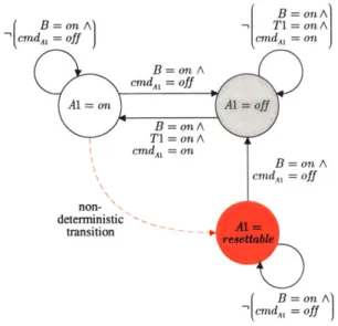
2.3.3 Amplifier Model

As illustrated in Figure 2-6, in addition to having on and off states, Amplifier #1 includes a repairable failure state (Al = resettable). This state captures situations in which a failed amplifier can be repaired simply by turning it off and then back on. For example, when the state of the power amplifier becomes uncertain due to observed off-nominal behavior, spacecraft operators would restore the nominal behavior of the amplifier by resetting it. In the case of the Mars Polar Lander's SSPA, the engineers found that if the RF output power drops below the required level, cycling the power off and on solves the problem [10]. Inclusion of this state will help demonstrate the reactive planner's ability to repair in the upcoming chapters.

Due to the interdependency between Transmitter #1 and Amplifier #1, the transition from off to on is conditioned on the Bus Controller being on, Transmitter #1 also being

on, and Amplifier #1 being commanded on (B = onAT1 = off AcmdAl = on). Otherwise,

the amplifier remains in the off state. Since turning the amplifier off does not have any harmful effects on any downstream components, turning the amplifier off from the on state only requires the Bus Controller to be on and the amplifier to be commanded off

(34)

B = on A (B = on A) ,T1=onA ,[cmdA, = off cmd,~ = on B = on A cmdc, = off A1l on A1=off B = on A cmd~l= onB _{= on A} cmd = off non_ determnistic transition-(B = on A ~cmdA, = off

Figure 2-6: Simplified model of Amplifier #1.

(B = on A cmdAl = off). For the same reason, the computer can turn the amplifier

off from the resettable state if B = on A cmdAl = off. Note that from the on state, the amplifier can non-deterministically fail to the resettable state at any time without the need to satisfy any constraints. Such non-deterministic unconstrained transitions are typical of failures, which generally occur unexpectedly.

Again, the model of the Amplifier #2 is exactly the same as Figure 2-6 except that T1, Al, and cmdT are replaced by T2, A2, and cmdT2, respectively.

2.3.4 Antenna Model

A lowgain antenna (LGA) is a passive device consisting of two possible states, nominal

and failed (see Figure 2-7). The nominal state is the operational state of the antenna. The failed state represents the unknown faulty state of the antenna. Although the antennas themselves serve no purpose in demonstrating commanding and repair, they will be used to demonstrate the reactive planner's capability to reconfigure the system quickly back to an operational state when an irreparable failure occurs. For example, assume that the Transmitter, Amplifier, and Antenna #1 are being used for downlink. If Antenna

(35)

Figure 2-7: Simplified model Antenna #1.

Amplifier #2 to maintain downlink capability.

(36)

(37)

Chapter 3 Symbolic Representation of

Concurrent Automata

A central idea in the model-based programming paradigm is the notion of an executable

specification [29]. In an executable specification, the system behavioral description is used directly for reactive planning. Thus, the conceptual description of the system be-havior must be written in, or automatically mapped to, some form of model on which deductive algorithms can operate. Furthermore, the computational model must be ca-pable of representing complex behaviors of a system while facilitating computationally tractable reactive planning.

Within the model-based execution framework, the behavior of the system being con-trolled is modelled as a factored partially observable Markov decision process (POMDP) that is compactly encoded as probabilistic concurrent constraint automata (CCA) [30]. Concurrency is used to model the behavior of a set of components that operate syn-chronously. Constraints are used to represent co-temporal interactions and intercommu-nication between components. Probabilistic transitions are used to model the stochastic behavior of components, such as failure.

While compact, this representation is also expressive enough to facilitate both mode estimation and reconfiguration. For the purpose of reactive planning, however, only a subset of the full CCA model is necessary, corresponding to state and control variables and transition functions. The constraints on dependent variables are eliminated by sub-stituting them with entailed constraints on state and control variables. The essential elements of the CCA model are extracted using knowledge compilation methods [31]

(38)

and encoded as concurrent automata (CA) for reactive planning. In essence, CA rep-resent a nondeterministic transition system with finite state and concurrently operating components. Compiling a CCA into a CA eliminates the need for constraint-based rea-soning. Also, the elimination of the dependent variables reduces the size of the state space. For example, the Deep Space One (DS1) CCA model developed for the Remote Agent included approximately 3000 propositional variables; with the dependent variables eliminated, only about 100 variables remained.

Regardless of the compactness of this representation, the exponential state space explosion problem pointed out by Ginsberg [18] still remains for reactive planning. This problem is addressed by leveraging the transition-based decomposition and the compact state space encoding capability of Ordered Binary Decision Diagrams (OBDD), i.e., a symbolic encoding. OBDD-based model checking [8] and OBDD-based universal planning

[11, 13, 12, 21] have proven particularly successful in dealing with the state explosion

problem. This problem can be mitigated for reactive planning by encoding CA as OBDDs, similar to how a typical automaton is encoded in an OBDD [7]. Once CA is represented using OBDDs, the planning algorithms can be defined in terms of OBDD operators.

In this chapter, a formal description of the CA computational model is introduced. Then, after a brief introduction to OBDDs, the OBDD representation of CA is discussed. Examples based on the simplified telecommunication system discussed in Chapter 2 are interleaved throughout this chapter.

3.1 Computational Model: Concurrent Automata

CA denote a set of concurrently operating automata. Though the CA model has not yet been formally introduced, the models of the simplified telecommunication system depicted in Section 2.3 (see Figures 2-4, 2-5, 2-6, and 2-7) are, in fact, graphical repre-sentations of the system's CA. In this section, the automaton for a single component is first formally defined, then CA is defined as a set of such automata. These definitions are similar to the definition of a CCA [30, 31, 29].

(39)

3.1 Computational Model: Concurrent Automata

3.1.1 Automaton Definition

Each automaton has an associated state variable si with domain D(si). Given the current state assignment (si = v), an automaton transitions its state in the next time step, according to a transition function ri. A transition function may be conditioned on a constraint involving the state of other automata and/or values of control variables. A transition is enabled if its constraint is entailed. In general, the domain of all control variables includes the default noCmd (i.e., no command) value. Formally, the automaton is defined as follows:

Definition 3.1. The automaton As for component i is a 4-tuple (Hi, Ei, -r, oM0_{3), where:}

1. Hi = H; U Hf is a finite set of variables for the component, where each variable

x E Hi ranges over a finite domain D(x). Hi is partitioned into a set of control variables H1 and a set of state variables H that includes the component's state variable si and possibly other sys.

2. E is a finite set of full assignments over Hs. A state of the automaton, denoted o-3, is an assignment to the component state variable si (i.e., og = (si = v)), where

si E fI and v E D(si). The state space of the component is the set E' C Ei, the projection of Ei to variable si. E C Ei is the projection of Ei to Uf.C

3. ri : Ei x C (He) -* 2E' is a transition function. C(Hi) denotes the set of all finite domain constraints over Us. A constraint is defined using propositional state

logic, in which a proposition is an assignment to a variable (x = v), or one of the constants true or false. Propositions are composed into a formula using the standard first-order logic operators: AND (A), OR (V), and NOT (-,). Given a

state assignment o(t) E Ei at time t and a constraint c) E C(H1) entailed at

time t, (, ct)) specifies a set of states to which the automaton can transition

at time t + 1. The transition function captures both nominal and fault behaviors, represented by ri" C ri and rf C -r, respectively. In the absence of fault behavior,

(40)

the nominal transition function is always deterministic (i.e., F : Ei x C(Hi) -+ Ei)

The fault transitions introduce nondeterminism into the system.

4. oO E E' is the initial state of the automaton.

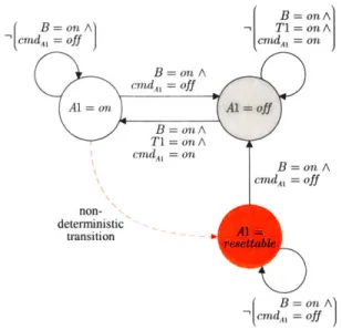
For example, consider Amplifier #1 illustrated once again in Figure 3-1. The au-tomaton is represented as 4-tuple (HAi, E1, TAl, ) where:

1. UA1 =

{B,

A1, Ti, cmdA1} is the set of variables, of which the state variable of Amplifier #1's component is Al. The variables are partitioned into a set of state variables Hi = {B, A1, Tl} and a set of control variables Hli =

{cmdAl}.

The domain of Al is D(A1) = {off, on,resettable}, and the domain of the remaining

variables are D(B) = D(Tl) = {off, on} and D(cmdAl) = {off, on, noCmd}.

2. While set EAi = D(B) x D(A1) x D(T1) x D(cmdAl) is too large to list, having 24 elements, the set of Amplifier #1 states (i.e., projection of EA1 to SAi) is El =

{A1 = off, Al = on, Al = resettable}, and the projection of EA1 to HAi is E'Ai =

{cmdAi = off, cmdAi = on}.

3. The set of constraints C(7Ai) associated with the transition function TAi is defined

in Equation 3.1.

(B= on A T1 = on A cmdAl = on), B = on A Ti = on A cndAl = on,

C(HAi) = , (B = on A cndAl = off), (3.1)

B = on A cmdAl = off,

The transition function TAi(UAi, CAi), where 0A1 E EA1 and CAi E C(HA1) is defined in Table 3.1.

(41)

3.1 Computational Model: Concurrent Automata B =on Al ~ cmdA = offj T1 = on A cmdAl = on B =on A , T1=onA cmd, = onI B = on A cmdA, = off non-deterministic transition B = on A -cmdI = off

Figure 3-1: Automaton of Amplifier #1 from the simplified telecommunication system.

qAl E EA1 Al = off Al = off Al = on Al = on Al = resettable Al = resettable

Table 3.1: Amplifier #1's Transition Function

CA1 E CA1

, (B = on A T1 = on A cmdAl = on) B on A T1 = on A cmdAl = on

(B = on A cmdAl = off) {A1 = on B = on A cmdAl =off {A1 = off

(B = on A cmdAl = off) {A1 B = on A cmdAl = off A1(OAl, CA1) [Al = off} {Al = on} , Al = resettablet} ,Al = resettablet} = resettable} {A1 = off }

tRepresents faulty behavior.

(42)

3.1.2 Concurrent Automata

CA is a set of concurrently operating automata. The simplified telecommunication sys-tem's CA consists of seven automata, one for each modelled component (i.e., Bus Con-troller, Transmitter #1 and #2, Amplifier #1 and #2, and Antenna #1 and #2). Within

this formalism, all automata are assumed to operate synchronously, that is, at each time step every component performs a single state transition. In this section, CA and its legal

execution are formally defined.

Definition 3.2. CA is a 3-tuple (A, H, E), where A = {A 1, A2,... ,,A} is a finite set

of automata associated with the n components in the system. H = H U J" ' is the set

of system variables, where each variable x E H ranges over a finite domain D(x). H is partitioned into a set of control variables flc =

Ul

₁ I and a set of state variables

Uls =

Un=

₁Hr. E =

fJ>

E, is a finite set of full assignments over Hi.

The state space of CA, denoted Es, is the Cartesian product of the individual au-tomaton state spaces E" , for all automata A, E A. The state of the system at time t, ( E , is

Un

₁ 0 , where (t) is the state of automaton A, at time t. Similarly, a

control action pi(t) E Ec is an assignment to all control variables, flc.

Definition 3.3. A legal execution of a CA is a trajectory of states [o( 0),a(1),...] and

control actions [I(0), p(, ...

]

such that:

1. o40) is an initial state of the system.

2. t+1 E U1Uri(o , c.) is the state of the system in the next time step t + 1,

for all c3 E C(HI) entailed by a(t) and 1().

The second part of the definition asserts that the next state, U(t+1), is defined by the transition functions {ri(oft, cj)|i = 1, 2,... , n}, where each transition is enabled by some

(43)

3.1 Computational Model: Concurrent Automata I'B =on A) A1 ₌ off _Al cmd₇, = off ,(cmdB = off) (a) B = on A ,I A1= offn cmdn = on B = on) (b)

Figure 3-2: Concurrent automata of (a) Bus Controller and (b) Transmitter #1.

nondeterministic behavior, the enabled transitions may lead to a set of possible states. Thus, 0(t+) is defined as one of those possible states, that is (t+1) E

1L=

₁U3 r-(uzt) c3).

For example, consider a subset of the simplified telecommunication system in which there are only three components: Bus Controller, Amplifier #1, and Transmitter #1. The graphical representations of the three concurrent automata are once again illustrated in Figures 3-2(a), 3-2(b), and 3-1, respectively. A state trajectory

{B = off,T1 = off,A1 = off}, {B = on,T1 = off,A1 = off},

{B = on,T1 = on,A1 = off},

{B = on, T1 = on, A1 = on},

(3.2)

and a sequence of control actions:

{cmdB = {cmdB = {cmdB =

on, cmdT1 = noCmd, cmdAl = noCmd},

noCmd, cmdTl = on, cmdAl = noCmd},

noCmd, cmdTl = noCmd, cmdAl = on},

(3.3)

represent a legal execution. In this scenario, all components are initially off, {B = off, T1=

off, Al = off }, and one by one each component is turned on.

(44)

3.2 Symbolic Representation of

CA

The use of a symbolic encoding called Ordered Binary Decision Diagram (OBDD) for reactive planning is motivated by the exponential state space explosion problem. This problem is not exclusive to reactive planning, but it has been a major source of dis-couragement for research in this area. After all, responsiveness, the objective of reactive planning, is generally realized by trading off the required computational time for the memory space.

The state space explosion problem is obvious and can be observed even in a model as simple as the simplified telecommunication system. Of the seven components in the simplified telecommunication system, five components have two states and the remaining two components have three states. This means that the simplified telecommunication system has a total of 25 x 32 = 288 possible states, that is, the number of states in a

system is exponential in the number of components. To alleviate this problem, OBDDs are used to encode all variable assignments, E, as well as transitions, r, of a CA. OBDDs provide two distinct benefits: (1) a compact state space encoding and (2) operators that allow a state space to be searched without the need to enumerate all of the states explicitly.

Encoding CA using OBDDs involves representing each finite domain variable in H and the transition functions ri as OBDDs. In this section, OBDDs are briefly introduced for readers who are not familiar with this representation. Then, the method for encoding finite domain variables in OBDDs is presented, followed by the method for encoding the transitions. For a more detailed discussion of OBDDs, refer to Appendix A.

3.2.1 Ordered Binary Decision Diagram

An Ordered Binary Decision Diagram (OBDD) is a rooted, directed acyclic graph (DAG) representation of a Boolean function, where the set of Boolean variables are ordered sequentially. A Boolean function

f

: B" -+ B is an expression formed with Boolean variables, and Boolean operators, including, but not limited to, negation -, conjunction A, disjunction V, implication =>, and equivalence e, where B is the Boolean domain

(45)

3.2 Symbolic Representation of CA 45

{true,

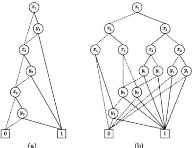
false}. Equation 3.4 is an example of a Boolean function.

(x1 Ay1)V (X2A y2) V (XsA y3) (3.4)

The corresponding OBDD with x₁ -< Y1 -< x2 -< Y2 -< x₃ -< y3 ordering is shown in

Figure 3-3(a). Each node of an OBDD represents a Boolean variable. The dotted and solid outgoing edges respectively represent false and true evaluations of the Boolean variable. The terminal nodes 1 and 0 represent the evaluation of the Boolean function (i.e., OBDD) where each path from the root to a terminal evaluates to 1 for true or 0 for false. The OBDD in Figure 3-3(a) has a total of five different paths from the root to terminal 1:

{x

1 = true, y1 = true}

{x1 = true, y1 = false,x2 = true, y2 = true}

{

x1 = f alse, x2 = true, Y2 = true} (3.5)

{xi = f alse,x2 = true, y2 = false,x3 = ture, y3 = ture}

{x

1 = false, x2 = false, x3 = true, y3 = true}

The fact that

{xi

= true, yi = true} terminates to 1 implies that as long as x1 = true and yi = true, Equation 3.4 evaluates to true regardless of the values of x2, X3, y2, and

Y3-The ordering of the variables is crucial to the compactness of an OBDD representation. For example, if the ordering of the same Boolean function in Equation 3.4 changes to

x1 < X2 -< x3 -< Y1 -< x2 -< y3, the size of the OBDD becomes considerably larger as shown in Figure 3-3. Unfortunately, determining an ordering that minimizes the size of the OBDD is a coNP-Complete problem [6]. However, ordering the "dependent" variables near each other is a good heuristic for reducing the size of an OBDD [14]. For example,

X1 Y1 - x₂-< Y2 -< X3 -< y3 places the "dependent" variables near each other. That is,

one possible solution of Equation 3.4 requires both x1 and y1 to be true, thus x1 and yi

are "dependent" on one another. Similarly, x2 and y2 are "dependent" on one another,

A decomposed symbolic approach to reactive planning

A DECOMPOSED SYMBOLIC APPROACH TO

REACTIVE PLANNING

@

SEP 1 0 2003

A Decomposed Symbolic Approach to

Reactive Planning

Abstract

Acknowledgments

Contents

List of Figures

List of Tables

Chapter 1

Introduction

1.1

Model-based Executive

1.2

Motivation for Tractable Reactive Planning

1.3

Thesis Contributions

1.3.1

Handling State Explosion through Decomposition

1.3.2

Handling State Explosion through Symbolic

Representa-tion

1.4

Thesis Outline

E*

Chapter 2

Spacecraft Telecommunication

System

2.1

MESSENGER Telecommunication System

[1].

2.2

Transmitter and Amplifier Interdependency

2.3

Simplified Telecommunication System

2.3.1

Bus Controller Model

2.3.2

Transmitter Model

2.3.3

Amplifier Model

2.3.4

Antenna Model

Chapter 3

Symbolic Representation of

Concurrent Automata

3.1

Computational Model: Concurrent Automata

3.1.1

Automaton Definition

{B,

{cmdAl}.

3.1.2

Concurrent Automata

Ul

Un=

fJ>

Un

]

1L=

3.2

Symbolic Representation of

CA

3.2.1

Ordered Binary Decision Diagram

f

{true,

{x

{

{x

{xi