Design Algorithms for Parallel Transmission
in Magnetic Resonance Imaging
by
Kawin Setsompop
M.Eng, Engineering Science
Oxford University, 2003
Submitted to the Department of Electrical Engineering and Computer Science
in Partial Fulfillment of the Requirements for the Degree of
Doctor of Philosophy
at the Massachusetts Institute of Technology
June 2008
© 2008 Massachusetts Institute of Technology
All rights reserved.
Author . . . .. . . . . .
Department of Electrical Engineering and Computer Science
May 2, 2008
Certified by. . .
Elfar Adalsteinsson
Robert J. Shillman Assistant Professor of Electrical Engineering and Computer
Science; Harvard-MIT Division of Health Science and Technology
Thesis Supervisor
Accepted by . . .
Terry P. Orlando
Chairman, Department Committee on Graduate Students
Design Algorithms for Parallel Transmission
in Magnetic Resonance Imaging
by
Kawin Setsompop
Submitted to the Department of Electrical Engineering
and Computer Science
on May 2, 2008, in Partial Fulfillment of the
Requirements for the Degree of
Doctor of Philosophy
Abstract
The focus of this dissertation is on the algorithm design, implementation, and validation of parallel transmission technology in Magnetic Resonance Imaging (MRI). Novel algorithms are proposed which yield excellent excitation control, low RF power requirements, methods that extend to non‐linear large‐flip‐angle excitation, as well as a new algorithm for simultaneous spectral and spatial excitation critical to quantification of low‐SNR brain metabolites in MR spectroscopic imaging. For testing and validation, these methods were implemented on a newly developed parallel transmission platform on both 3 T and 7 T MRI scanners to demonstrate the ability of these methods for high‐ fidelity B1+ mitigation, first by excitation of phantoms and then by human imaging.
Further, spatially tailored RF pulses were demonstrated beyond conventional slice‐ or slab‐selective excitation.
Thesis Supervisor: Elfar Adalsteinsson
Title: Robert J. Shillman
Assistant
Professor of Electrical Engineering and Computer
Science; Harvard-MIT Division of Health Science and Technology
Acknowledgements
This work would have not been possible without the help and support of many individuals.
First, most importantly, I would like to thank my advisor, Prof. Elfar Adalsteinsson, who has been instrumental to this work. It has been a pleasure working with him. I am grateful for his inputs, enthusiasm, support, and guidance. I have learned so much from our discussions, not just on MRI, but on the general approach towards ones work.
I am fortunate to have the opportunity to work with Prof. Larry Wald. He has helped me tremendously. I thank him for his input and his reasoned advice which has significantly improved the work in this thesis.
I thank Prof. Dennis Freeman, who kindly gave his time to serve on my thesis committee.
I am grateful to my main collaborator and friend, Vijay Alagappan, who has played an integral role in the research effort of this thesis. He built all the RF coil array hardware used in this work and has helped with the setup of all the experiments. There were countless weekends that we have shared together at the scanner, willing or not, tinkering with equipments, trying to make things work. Thanks for your patience and for putting up with me.
It has been a pleasure interacting and working with the students in the Magnetic Resonance Imaging Group. In particular, I would like to thank Borjan Gagoski, who has been there with me from the start. I thank him for his friendship, help, and technical collaboration. I would also like to thank Div Bolar, Padraig Cantillon‐Murphy, Joonsung Lee, Trina Kok, and Adam Zelinski.
I would like to express my appreciation to Arlene Wint who has made things run very smoothly for me and for the people in the lab.
I appreciate the help given to me by the students, and staff in the HST A. A. Martinos Center for Biomedical Imaging at MGH. In particular, I would like to thank Thomas Witzel, Dr. Jonathan Polimeni, and Dr. Graham Wiggins.
Siemens Medical Solution has provided both equipment and support that was essential for all the experiments in this thesis. The effort of Dr. Franz Schmitt, Ulrich
Fontius, Dr. Franz Hebrank, Dr. Andreas Potthast, and Dr. Juergen Nistler are especially appreciated.
I would like to acknowledge the financial support provided by the National Institutes of Health, NIBIB grants R01EB006847, R01EB007942, R01EB000790, and NCRR grant P41RR14075, Siemens Medical Solutions, R.J. Shillman Career Development Award, and the MIND Institute.
I wish to express my deepest appreciation for Chanikarn Wongviriyawong who has been such an integral part of my MIT experience. I thank her for her love, cheerful support, and encouragement that have kept me going for the last three years. I could not have found a truer companion through it all.
Finally, I would like to thank my parents, Wirote and Wandee, for their unconditional love and support. Without whom none of this would have been possible.
Massachusetts Institute of Technology
Kawin Setsompop
April 25, 2008
Contents
Acknowledgements ... 5
Contents ... 7
List of Figures ... 9
Introduction ... 15
Chapter 1 Background: RF Excitation in MRI ... 21
1.1 Magnetic Resonance Imaging ... 21
1.2. RF Excitation Pulse Design ... 24
1.2.1 Single Channel transmission Theory ... 25
1.2.2 Parallel Transmission Theory ... 30
1.3 Imaging Schemes for Contrast Generation ... 41
Chapter 2 Parallel RF Transmission at 3 Tesla... 49
2.1 Phantom experiments ... 49
2.1.1 Introduction ... 49
2.1.2 Methods ... 50
2.1.3 Results ... 57
2.1.4 Discussion ... 63
2.1.5 Conclusion ... 64
2.2 In Vivo Experiments ... 66
2.2.1 Introduction ... 66
2.2.2 Theory & Method ... 66
2.2.3 Results ... 68
2.2.4 Discussion and Conclusion ... 70
Chapter 3 Rapid Quantitative B1 mapping ... 71
3.1 Introduction ... 71
3.2 Theory ... 72
3.2.1 Saturated Double‐Angle method ... 72
3.2.2 Rapid Quantitative B1+ Mapping via Receive profile estimation ... 76
3.2.3 Experimental B1+ mapping ... 80
Chapter 4 Magnitude Least Square Optimization ... 83
4.1 Introduction ... 83
4.2 Theory ... 84
4.3 Methods ... 87
4.4 Results ... 91
4.5 Discussion ... 98
Chapter 5 In‐vivo Parallel Excitation at 7 Tesla ... 101
5.1 Introduction ... 101
5.2 Methods ... 101
5.3 Results ... 107
5.4 Discussion ... 118
5.5 Conclusion ... 119
Chapter 6 Spectral‐Spatial Parallel Excitation ... 121
6.1 Introduction ... 121
6.2 Theory ... 122
6.3 Method ... 123
6.4 Results ... 126
6.5 Discussion and Conclusions ... 132
Chapter 7 High‐Flip‐Angle Parallel Excitation ... 135
7.1 Introduction ... 135
7.2 Theory ... 136
7.3 Methods ... 142
7.4 Results ... 144
7.5 Discussion and Conclusions ... 148
Chapter 8 Summary and Recommendations ... 149
8.1 Summary ... 149
8.2 Recommendations ... 151
Bibliography ... 153
List of Figures
FIGURE1:RF EXCITATION AND SIGNAL GENERATION ... 23 FIGURE 2: EMPLOYING GRADIENT FIELD FOR SIGNAL ACQUISITION ... 24 FIGURE 3:SLICE-SELECTIVE EXCITATION; LEFT: TARGET EXCITATION AND ITS FOURIER TRANSFORM, RIGHT:
CORRESPONDING GRADIENT AND RF PULSES. ... 27 FIGURE 4:MIT LOGO TARGET EXCITATION PROFILE AND ITS TRANSFORM ... 28 FIGURE 5:2D EXCITATION DESIGN; TOP: TARGET’S FOURIER TRANSFORM AND SPIRAL K-SPACE TRAJECTORY,
BOTTOM: CORRESPONDING RF AND GRADIENT PULSES, AND THE RESULTING EXCITATION PROFILE. ... 28 FIGURE 6:SPOKES (LEFT) AND STACK OF SPIRAL (RIGHT) TRAJECTORIES. ... 29 FIGURE 7:CYLINDRICAL TARGET EXCITATION AND THE RESULTS OF SINGLE-CHANNEL ECHO PLANER
EXCITATION WITH 2X ACCELERATION LEADING TO ALIASING/WRAP-AROUND EFFECT ... 32 FIGURE 8:CYLINDRICAL EXCITATION (2X) VIA PARALLEL TRANSMISSION OF TWO ORTHOGONAL RF COILS
RESULTING IN NO ALIASING/WRAP-AROUND EFFECT ... 33 FIGURE 9:RF COIL ARRAYS EMPLOYED IN THIS WORK:(A) EIGHT-CHANNEL LOOP COIL ARRAY AT 3T,(B)
EIGHT-CHANNEL STRIPLINE ARRAY AT 7T,(C) SIXTEEN-CHANNEL STRIPLINE ARRAY AT 7T. ... 35 FIGURE 10:DIAGRAM OF THE BUTLER MATRIX WITH N/2 INPUTS FROM THE RF AMPLIFIERS AND N OUTPUTS
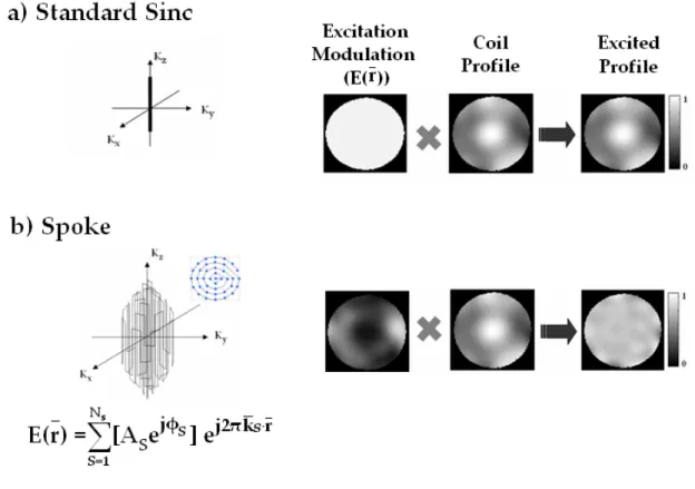
TO THE TRANSMISSION COIL ELEMENTS.THE POWER TRANSMITTED BY THE KTH AMPLIFIER IS SPLIT INTO EQUAL PARTS AND FEED TO THE OUTPUT WITH APPROPRIATE PHASE SHIFTS TO GENERATE THE KTH BIRDCAGE MODE. ... 37 FIGURE 11:SLICE-SELECTIVE B1+ MITIGATED EXCITATION VIA SINGLE CHANNEL RF, A)STANDARD SLICE
-SELECTIVE SINC EXCITATION WITH NO IN-PLANE MODULATION, RESULTING IN LARGE VARIATION IN THE EXCITED PROFILE. B)SPOKE EXCITATION WITH SUFFICIENT IN-PLANE MODULATION TO CORRECT FOR SEVERE B1+ INHOMOGENEITY. ... 39 FIGURE 12:ACCELERATION OF SPOKE TRAJECTORY VIA PARALLEL EXCITATION RESULTING IN A
SIGNIFICANTLY REDUCTION IN THE NUMBER OF REQUIRED SPOKES, AND HENCE EXCITATION DURATION. ... 41 FIGURE 13:(A)BASIC SATURATION-RECOVERY SEQUENCE:A STRING OF 90° EXCITATION PULSES
SEPARATED BY REPETITION TIME TR, ALONG WITH DATA ACQUISITION (REPRESENTED BY THE BLACK BLOCKS) AFTER EACH EXCITATION AT THE GRADIENT ECHO TIME TE. (B) TIME COURSE OF MZ: VALUE OF MZ PRIOR TO THE 90° PULSE DETERMINES THE RESULTANT SIGNAL GENERATED.FIGURE ADAPTED FROM (18). ... 42 FIGURE 14:SPIN ECHO GENERATION:AFTER THE 90° EXCITATION (A)-(B), DUE TO LOCAL FIELD VARIATION
THE TRANSVERSE MAGNETIZATION OF THE DIPOLE MOMENTS ROTATE AT SLIGHTLY DIFFERENT FREQUENCY RESULTING IN PHASE DISPERSION (C).THE PHASE DISPERSION IS NEGATED WITH A 180°
PULSE APPLIED ALONG THE X-AXIS (D), CAUSING THE DIPOLE MOMENTS TO REPHRASE AFTER TIME
τ
.FIGURE ADAPTED FROM (18). ... 45 FIGURE 15:SATURATION-RECOVERY SEQUENCE WITH SPIN ECHOES.FIGURE ADAPTED FROM (18). ... 45 FIGURE 16: A)SIEMENS 3T PARALLEL TRANSMISSION SCANNER. B)EIGHT-CHANNEL COIL ARRAY.EACH COIL
HAS 17 CM DIAMETER, AND PLACED IN AN OVERLAPPING PATTERN ON AN ACRYLIC CYLINDER WITH A
28 CM DIAMETER.CENTERED IN THE COIL IS A 17-CM DIAMETER OIL-FILLED SPHERICAL PHANTOM THAT WAS USED FOR EVALUATION OF THE PARALLEL RF EXCITATION DESIGNS. ... 51 FIGURE 17:DURATION OF RF PULSE DESIGN FOR THE HIGH-RESOLUTION IN-PLANE EXCITATION DESIGN AS A
FUNCTION OF ACCELERATION FACTOR. ... 52 FIGURE 18: K-SPACE TRAJECTORY FOR THE 4 SPOKES DESIGN (LEFT) AND FOR THE 7 SPOKES DESIGN (RIGHT)
FIGURE 19:MAGNITUDE (TOP) AND PHASE (BOTTOM) OF THE COIL PROFILES.COIL 1 IS ON THE LEFT, COIL 2
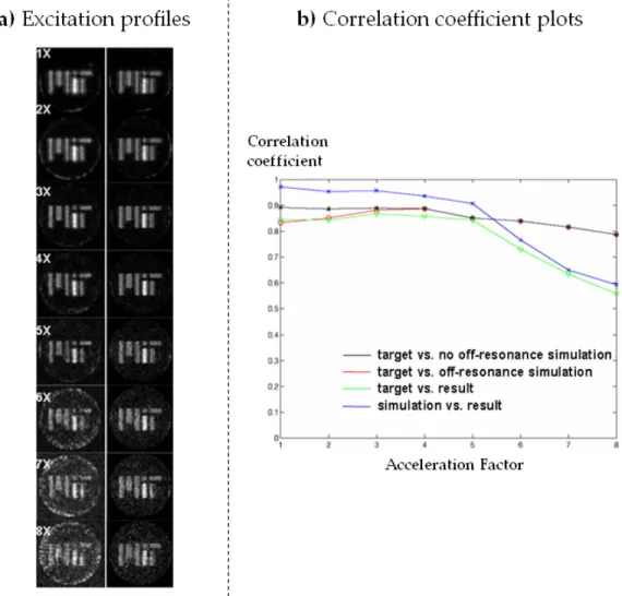
IS AT 45º CLOCKWISE TO COIL 1, AND SO ON FOR EACH OF THE 8 COILS. ... 57 FIGURE 20: A)MAGNITUDE OF 2D EXCITATION WITH 1X THROUGH 8X ACCELERATION.EXPERIMENTAL
DATA ARE SHOWN ON THE LEFT, AND SIMULATIONS ON THE RIGHT BASED ON THE MEASURED B1+ MAPS.
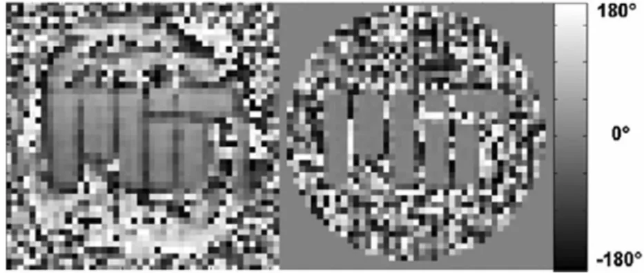
B)PLOT OF CORRELATION COEFFICIENTS AMONG ACQUIRED, SIMULATION, AND TARGET PROFILE AS A FUNCTION OF ACCELERATION FACTOR FOR THE 2D EXCITATION. ... 58 FIGURE 21:PHASE OF 2D EXCITATION DESIGN FOR 4X ACCELERATION, ACQUIRED DATA ON THE LEFT,
SIMULATION ON THE RIGHT. ... 59 FIGURE 22:EXPERIMENTAL RESULTS, FOR THE 2D EXCITATION AT 4X ACCELERATION WITH MISSING
CHANNEL(S) ARE SHOWN ON THE LEFT.EVEN WITH ONE CHANNEL MISSING SEVERE ARTIFACTS ARE APPARENT.ALSO DEPICT ARE THE SIMULATION OF THE PROFILES THAT WOULD HAVE BEEN CREATED BY EACH COIL IN THIS EXPERIMENT. ... 60 FIGURE 23:INCREASED EXCITATION VOLTAGE FOR A 4X ACCELERATION DESIGN WITH 2D EXCITATION
DEMONSTRATES THE INCREASED SNR WITH HIGHER VOLTAGE, BUT AT THE SAME TIME, INCREASED THE CANCELLATION ARTIFACTS IN THE BACKGROUND OF THE SPHERICAL PHANTOM DUE TO VIOLATION OF THE SMALL TIP ANGLE APPROXIMATION. ... 60 FIGURE 24: SHOWS THE RESULTS AND SIMULATION DATA FOR THE 4 SPOKES (LEFT) AND THE 7 SPOKES
(RIGHT) DESIGNS.IN EACH OF THE TWO SUB-FIGURES, THE TOP LEFT AND RIGHT ARE THE IN-PLANE AND SLICE SELECTION PROFILES OF RESULTS.THE BOTTOM LEFT IS THE Y-SLICES IN-PLANE PROFILES OF RESULT, AND THE BOTTOM RIGHT IS IN-PLANE DATA FROM THE SIMULATION. ... 62 FIGURE 25:SIMULATION OF STANDARD SLICE-SELECTIVE (TOP) AND RF SHIMMING (BOTTOM) EXCITATIONS.
IN EACH OF THE TWO SUBFIGURES THE LEFT PANEL DISPLAYS THE OVERALL IN-PLANE PROFILE, AND THE RIGHT PANEL SHOWS A SERIES OF IN-PLANE PROFILES. ... 62 FIGURE 26:B1+ MAP ESTIMATION:3-RD ORDER POLYNOMIAL IS USED TO REMOVED THE ANATOMY AND
SMOOTH THE MAGNITUDE PROFILE (TOP),B0 MAP IS USED TO REWIND THE PHASE OF THE PHASE PROFILE (BOTTOM) ... 67 FIGURE 27:A) AN 8-CHANNEL EXCITATION BODY ARRAY SYSTEM,B) AN 8-CHANNEL EXCITATION HEAD
ARRAY SYSTEM. ... 68 FIGURE 28:A)BODY-ARRAY EXCITATION:B0 MAP (TOP-LEFT) SHOWS LARGE INHOMOGENEITY IN THE
FRONTAL SINUS AREA, SLICE-SELECTIVE EXCITATION WITHOUT (TOP-RIGHT) AND WITH (BOTTOM-LEFT) B0 CORRECTION.SLICE PROFILE IS ALSO SHOWN (BOTTOM-RIGHT).B)HEAD-ARRAY EXCITATION:2X
ACCELERATION “TIM TX”EXCITATION WITHOUT (RIGHT) AND WITH (CENTER)B0 CORRECTION.4X
ACCELERATION “HALF BRAIN” EXCITATION WITHOUT B0 CORRECTION (LEFT). ... 69
FIGURE 29:THE RESET PULSE SEQUENCE USED IN SATURATED DOUBLE-ANGLE METHOD.SEQUENCE DIAGRAM IN (A) SHOWS THE SATURATION PULSE (MZRESET) BEING APPLIED AFTER EACH DATA ACQUISITION TO SATURATE MZ PRIOR TO THE NEXT EXCITATION.THE MZ TIME COURSE OF THIS SEQUENCE IS SHOWN IN (B). ... 74
FIGURE 30:FLOWCHART OUTLINING THE RAPID QUANTITATIVE B1+ MAPPING TECHNIQUE, WHERE FIRST RECEIVE PROFILE OF THE RECEPTION COIL IS ESTIMATED IN STEP 1-5, AFTER WHICH B1+ MAPS OF THE TRANSMIT COILS (OR MODES) CAN THEN BE OBTAIN VIA STEP 6-7. ... 79 FIGURE 31: A)EIGHT-CHANNEL TRANSMIT/RECEIVE STRIPLINE COIL ARRAY FOR 7T.THE INSERT ON THE
RIGHT PANEL OF A) SHOWS THE ESTIMATED TRANSMIT (TX) AND RECEIVE (RX) PROFILES AND THE TRANSMIT-RECEIVE IMAGE (TX-RX) OF THE CP MODE OF THE ARRAY FOR A WATER-FILLED SPHERICAL PHANTOM PLACED INSIDE A LOADING RING. B)THE UPPER PANEL SHOWS ESTIMATED MAGNITUDE
(INTENSITY SCALE NORMALIZED TO A MAXIMUM VALUE OF 1), AND THE LOWER PANEL SHOWS PHASE
(DEGREES) OF THE INDIVIDUAL EXCITATION COIL PROFILES. ... 81 FIGURE 32: A)SIXTEEN-CHANNEL TRANSMIT/RECEIVE STRIPLINE COIL ARRAY FOR 7T, AND THE BUTLER
MATRIX HARDWARE THAT WAS USED FOR THE EXPERIMENTS IN THIS WORK.THE INSERT ON THE RIGHT PANEL OF A) SHOWS THE ESTIMATED TRANSMIT (TX) AND RECEIVE (RX) PROFILES AND THE
TRANSMIT-RECEIVED IMAGE (TX-RX) OF THE CP MODE OF THE ARRAY FOR A WATER-FILLED SPHERICAL PHANTOM. B)THE UPPER PANEL SHOWS THE ESTIMATED MAGNITUDE PROFILE (INTENSITY SCALE NORMALIZED TO A MAXIMUM VALUE OF 1), AND THE LOWER PANEL SHOWS THE PHASE PROFILE
(IN DEGREES) OF THE EIGHT ORTHOGONAL BIRDCAGE TRANSMISSION MODES USED. ... 81
FIGURE 33:FLOW DIAGRAM OF THE MODIFIED LOCAL-VARIABLE EXCHANGE METHOD FOR MAGNITUDE
LEAST SQUARE OPTIMIZATION.DURING THE ITERATIVE OPTIMIZATION PROCESS, A SMOOTHED VERSION OF THE EXCITATION PHASE FROM THE PREVIOUS ITERATION IS USED AS THE TARGET
EXCITATION PHASE FOR THE CURRENT ITERATION.THE SMOOTHING OF THE EXCITATION PHASE PROFILE IS PERFORMED USING A DESIGNER-SPECIFIED GAUSSIAN FILTER, ENABLING THE DESIGNER TO SYSTEMATICALLY TRADE OFF THE ALLOWED SPATIAL PHASE VARIATION FOR AN IMPROVEMENT IN THE MAGNITUDE PROFILE AND REDUCTION IN RF POWER. ... 87 FIGURE 34:EIGHT-CHANNEL TRANSMIT/RECEIVE STRIPLINE COIL ARRAY FOR 7T THAT WAS USED FOR ALL
EXPERIMENTS IN THIS CHAPTER.THE INSERT ON THE RIGHT PANEL OF A) SHOWS THE ESTIMATED TRANSMIT (TX) AND RECEIVE (RX) PROFILES AND THE TRANSMIT-RECEIVED IMAGE (TX-RX) OF THE BIRDCAGE MODE OF THE ARRAY FOR A WATER-FILLED SPHERICAL PHANTOM PLACED INSIDE A LOADING RING.ALSO SHOWN IS AN EXAMPLE OF THE TRANSMIT-RECEIVED IMAGE (TX-RX) OF THE BIRDCAGE
MODE OF THE ARRAY FOR AN AXIAL BRAIN SECTION THAT DEMONSTRATES COMPARABLE
INHOMOGENEITY TO THE TRANSMIT-RECEIVED IMAGE OF THE PHANTOM. ... 89 FIGURE 35: A)EXPERIMENTAL SQUARE-TARGET EXCITATION, IMAGED IN A CENTRAL AXIAL SECTION OF A
3D-ENCODED READOUT.THE FIGURE ILLUSTRATES THE EXCITATION MAGNITUDE PROFILE IMPROVEMENT WITH THE MAGNITUDE LEAST SQUARES DESIGN WHEN COMPARED TO THE
CONVENTIONAL LEAST SQUARES DESIGN FOR THE TIKHONOV REGULARIZATION PARAMETER VALUE OF
1.5.THE TOP ROW COMPARES THE OVERALL EXCITATION.THE WINDOW AND LEVEL PARAMETERS FOR THE SECOND ROW ARE SET TO BRING OUT THE BACKGROUND NOISE, AND THE THIRD ROW IS WINDOWED TO BEST COMPARE THE INTENSITY VARIATION WITHIN THE SQUARE TARGET EXCITATION. B)PLOT OF NORMALIZED RMMSE VS.RF VOLTAGE NORM ACROSS ALL 8 CHANNELS ( b 2), FOR FOUR DIFFERENT SETTINGS OF THE TIKHONOV REGULARIZATION PARAMETER (L-CURVE). ... 93 FIGURE 36:EXPERIMENTAL SQUARE-TARGET EXCITATION FOR A FIXED VALUE OF TIKHONOV
REGULARIZATION PARAMETER (
β
=1.5), MAGNITUDE (LEFT) AND PHASE (RIGHT) BY, A)CONVENTIONAL LEAST-SQUARES OPTIMIZATION, AND B) BY MAGNITUDE LEAST SQUARES.LARGER VARIATION OF SPATIAL PHASE PROFILE IS OBSERVED FOR THE MAGNITUDE LEAST SQUARES DESIGN AS EXPECTED.ADDITIONALLY, THE MLS DESIGN YIELDS BETTER TARGET EXCITATION AND BACKGROUND SUPPRESSION WITHIN THE PHANTOM OUTSIDE THE TARGET SQUARE.PANEL C) SHOWS A ZOOMED REGION OF THE PHASE PROFILE FROM THE MLS DESIGN, AND SHOWS THE HIGH DEGREE OF SIMILARITY BETWEEN EXPERIMENTAL (LEFT) AND SIMULATION RESULTS (RIGHT). ... 94 FIGURE 37: A)& B)ACQUIRED DATA AND SIMULATION RESULTS FOR A 4-SPOKE EXCITATION BY
CONVENTIONAL LEAST-SQUARES (A), AND MAGNITUDE LEAST SQUARES (B), FOR THE TIKHONOV REGULARIZATION PARAMETER PAIR THAT RESULTED IN THE LOWEST EXPERIMENTAL RMMSE.IN EACH PANEL, THE TOP ROW SHOWS THE EXPERIMENTAL IN-PLANE AND THROUGH-SLICE PROFILES,
WHILE THE LOWER RIGHT IMAGE SHOWS THE PREDICTED PROFILE BASED ON A BLOCH-EQUATION SIMULATION OF THE RF WAVEFORMS.THE BOTTOM LEFT FIGURE IN EACH PANEL SHOWS SEVERAL SECTIONS THROUGH THE IN-PLANE PROFILE. C)L-CURVE PLOT OF THE NORMALIZED RMMSE VS.RF VOLTAGE NORM ACROSS ALL 8 CHANNELS ( b 2), FOR SIX DIFFERENT SETTINGS OF THE TIKHONOV REGULARIZATION PARAMETER. ... 96 FIGURE 38:EXPERIMENTAL MAGNITUDE (LEFT) AND PHASE (RIGHT) RESULTS FOR A 4-SPOKES EXCITATION
BY CONVENTIONAL LEAST-SQUARES (A), AND MAGNITUDE LEAST SQUARES (B), FOR THE TIKHONOV REGULARIZATION PARAMETER PAIR THAT RESULTED IN THE LOWEST EXPERIMENTAL RMMSE.
LARGER VARIATION OF SPATIAL PHASE PROFILE IS OBSERVED FOR THE MAGNITUDE LEAST SQUARES DESIGN AS EXPECTED.ADDITIONALLY, THE MLS DESIGN YIELDS A MUCH MORE UNIFORM MAGNITUDE PROFILE.PANEL C) SHOWS A ZOOMED PHASE SCALING VERSION OF THE PHASE PROFILE FROM THE MLS
DESIGN, AND SHOWS THE HIGH DEGREE OF SIMILARITY BETWEEN EXPERIMENTAL (LEFT) AND
SIMULATION RESULTS (RIGHT). ... 97 FIGURE 39: A)PROFILES FOR COMBINED TX-RX, ALONG WITH ESTIMATES OF THE SEPARATE TX AND RX OF
THE MODE-1 BIRDCAGE OF THE COIL FOR A HEAD SHAPED PHANTOM, AND B) HUMAN BRAIN (SUBJECT
1). ...102 FIGURE 40:MAGNITUDE (TOP) AND PHASE (BOTTOM)B1+ MAPS OF THE 8 OPTIMAL MODES FOR A) THE HEAD
-SHAPED PHANTOM, AND B) AN AXIAL SECTION IN HUMAN BRAIN (SUBJECT 1). ...104 FIGURE 41:THE OPTIMIZED THREE (A) AND TWO-SPOKE (B) K-SPACE TRAJECTORIES FOR THE PULSE DESIGN IN
THE HEAD-SHAPED PHANTOM AND HUMAN EXCITATION EXPERIMENT RESPECTIVELY.THE OPTIMIZED TWO-SPOKE PLACEMENTS IN (KX,KY) FOR THE IN THE IN VIVO EXPERIMENTS VARIED SLIGHTLY FROM SUBJECT TO SUBJECT, BUT IN ALL CASES WERE TWO-SPOKE DESIGNS. ...105
FIGURE 42:HEAD-SHAPED WATER PHANTOM B1+MITIGATION.FLIP-ANGLE MAPS AND LINE PROFILES FOR: A)
BIRDCAGE MODE WITH CONVENTIONAL 1-MS LONG SINC SLICE-SELECTIVE EXCITATION,
DEMONSTRATING A 1:6.8 MAGNITUDE VARIATION WITHIN THE FIELD-OF-EXCITATION (FOX); B)RF
SHIMMING,1 MS-LONG PULSE, DEMONSTRATING A SUBSTANTIAL RESIDUAL FLIP-ANGLE
INHOMOGENEITY AS MEASURED BY THE RESIDUAL STANDARD DEVIATION AND THRESHOLD METRICS;
AND, C) THREE-SPOKE MLS, SLICE-SELECTIVE 2.4-MS LONG PULSE, DEMONSTRATING EXCELLENT MITIGATION OF THE B1+ INHOMOGENEITY. ...109
FIGURE 43:COMPARISON OF B1+ MITIGATION BY A) A LEAST-SQUARES, AND B) A MAGNITUDE-LEAST
-SQUARES 3-SPOKE RF DESIGN WITH THE SAME K-SPACE TRAJECTORY (2.4 MS) AND PULSE SHAPE (SINC, TIME-BANDWIDTH PRODUCT=4) AS DEMONSTRATED ON A HEAD-SHAPED WATER PHANTOM WITH SUBSTANTIAL TX INHOMOGENEITY.ON THE LEFT IS A BLOCH SIMULATION OF THE MAGNITUDE AND PHASE PROFILES, ON THE RIGHT ARE EXPERIMENTAL RESULTS WITH LINE PROFILES THROUGH THE MAGNITUDE IMAGE.ALSO SHOWN, BOTTOM RIGHT, IS THE EXCITATION PHASE PROFILE. ...110 FIGURE 44:COMPARISON OF PHASE DUE TO THE EXCITATION ONLY (LEFT) AND PHASE MEASURED IN A
GRADIENT ECHO AT TE=5MS, WHICH ALSO INCLUDES THE ACCRUAL OF PHASE DUE TO B0
INHOMOGENEITY (CENTER).THE B0(X,Y) TERM IS ACCORDING TO A SEPARATELY ESTIMATED B0
FIELDMAP (RIGHT).CLEARLY, THE EXCITATION PHASE VARIATION RESULTING FROM THE MLS DESIGN IS VERY SMALL COMPARED TO THE ACCRUED PHASE DUE TO B0 INHOMOGENEITY AT TE=5MS, AND IS
SLOWLY VARYING OVER THE FOX, AND THUS DOES NOT INTRODUCE ANY INTRA-VOXEL DEPHASING. ...111 FIGURE 45:B1+ MITIGATION COMPARISON FOR SUBJECT 1.THE COMPARISON INCLUDES SLICE SELECTION
BASED ON MODE-1 BIRDCAGE (TOP ROW),RF SHIMMING (CENTER ROW), AND TWO-SPOKE (BOTTOM ROW) EXCITATION PULSES.ON THE LEFT OF EACH ROW IS THE IN-PLANE IMAGE OF THE EXCITED SLICE AFTER THE REMOVAL OF THE RECEIVE PROFILE.ON THE RIGHT IS THE FLIP-ANGLE MAP ESTIMATE,
ALONG WITH THE LINE PROFILE PLOTS. ...113 FIGURE 46:B1+ MITIGATION COMPARISON FOR SUBJECT 5, WHO HAS THE MOST SEVERE B1+ VARIATION (IN
THE MODE-1 BIRDCAGE EXCITATION) OUT OF ALL THE SIX SUBJECTS. ...114 FIGURE 47:TWO-SPOKE EXCITATION FOR SUBJECT 4 WITH A 3D READOUT. A)SLICE PROFILE PLOT, WHERE
THE SOLID LINE REPRESENTS THE PREDICTED PROFILE AND THE CIRCLES REPRESENT THE
EXPERIMENTAL DATA.EACH DATA POINT ALONG THE SLICE PROFILE REPRESENTS THE AVERAGE IN
-PLANE INTENSITY AT THAT PARTICULAR Z-LOCATION. B)IN-PLANE IMAGES (A)-(J), AT 1-MM
SEPARATION ALONG Z, OVER A 1-CM RANGE AROUND THE 0.5-CM EXCITED SLICE. ...117 FIGURE 48: K-SPACE TRAJECTORY FOR THE 4-SPOKES EXCITATION IS SHOWN ON THE LEFT.ON THE RIGHT ARE
THE RF WAVEFORM FOR ONE OF THE EIGHT TRANSMISSION MODES (MODE 1), AND THE GRADIENT WAVEFORMS THAT WERE USED FOR THE EXCITATION. ...124 FIGURE 49:IN-PLANE EXCITATION PROFILES AT CENTER FREQUENCY FOR RF SHIMMING, CONVENTIONAL
SPOKE, AND SPECTRAL-SPATIAL SPOKE EXCITATIONS RESPECTIVELY. ...127
FIGURE 50:STANDARD DEVIATION PLOTS COMPARING A) THE SIMULATED PERFORMANCE OF THE THREE TYPES OF EXCITATION DESIGNS, AND B) THE SIMULATED AND EXPERIMENTAL PERFORMANCE OF THE SPECTRAL-SPATIAL SPOKE EXCITATION DESIGN OVER A ±500HZ FREQUENCY RANGE. ...128 FIGURE 51:EXCITATION PERFORMANCE ACHIEVED BY THE SPECTRAL-SPATIAL PULSE AT 300HZ OFF
-RESONANCE WITH THE THROUGH-SLICE PROFILE (TOP), THE IN-PLANE PROFILES AT 3 DIFFERENT THOUGH PLANE POSITIONS ALONG THE EXCITED SLAB (CENTER), AND THE CORRESPONDING 1-D
PROFILES AT SEVERAL CUTS THROUGH THE IN-PLANE PROFILES (BOTTOM).EXCELLENT SLICE
SELECTION AND GOOD IN-PLANE PROFILES CAN BE OBSERVED. ...130
FIGURE 52:SUMMARIZES THE EXCITATION PERFORMANCE ACHIEVED BY THE SPECTRAL-SPATIAL PULSE AT 0 HZ OFF-RESONANCE.EXCELLENT SLICE SELECTION AND GOOD IN-PLANE PROFILES CAN BE OBSERVED. ...130 FIGURE 53:SUMMARIZES THE EXCITATION PERFORMANCE ACHIEVED BY THE SPECTRAL-SPATIAL PULSE AT
-300HZ OFF-RESONANCE.EXCELLENT SLICE SELECTION AND GOOD IN-PLANE PROFILES CAN BE OBSERVED. ...131 FIGURE 54:FROM LEFT TO RIGHT: THE MAGNITUDE AND PHASE PROFILES FOR THE CENTER SLICE OF THE
EXCITED SLAB AT -200,0, AND +200HZ RESPECTIVELY.THE MAGNITUDE PROFILE EXHIBITS GOOD UNIFORMITY AT ALL THREE FREQUENCIES WHILE, AS EXPECTED FROM THE MLS OPTIMIZATION, THE PHASE PROFILE VARIES SMOOTHLY BOTH SPATIALLY AND SPECTRALLY. ...131
FIGURE 55:EXCITATION PROFILES FROM THE 3-SPOKE 90° EXCITATION,LEFT: THE IN-PLANE AND THE SLICE SELECTION PROFILES,RIGHT: THE 1-D THROUGH-PLANE PROFILES ALONG SEVERAL CUTS THROUGH THE IN-PLANE PROFILE. ...145 FIGURE 56:SIMULATION AND EXPERIMENTAL DATA PLOTS OF THE NORMALIZED AVERAGE IN-PLANE
INTENSITY AS A FUNCTION OF PEAK RF VOLTAGE FOR THE 3-SPOKES 90° EXCITATION.GOOD
AGREEMENT BETWEEN THE SIMULATION AND EXPERIMENTAL DATA CAN BE OBSERVED. ...145 FIGURE 57:Z-GRADIENT (GZ) AND RF WAVEFORMS FROM ONE OF THE EXCITATION COIL (COIL 1) FOR THE
VERSED SPIN-ECHO SEQUENCE CONSISTING OF A 3-SPOKE 90° AND180° SPIN-ECHO EXCITATIONS (TE =20 MS).ALSO SHOWN ARE THE GZ CRUSHER GRADIENTS SURROUNDING THE SPIN-ECHO RF. ...146
FIGURE 58:SPIN-ECHO EXCITATION PROFILES,LEFT: THE IN-PLANE AND THE SLICE SELECTION PROFILES,
RIGHT: THE 1-D THOUGH-PLANE PROFILES ALONG SEVERAL CUTS THROUGH THE IN-PLANE PROFILE. ...147 FIGURE 59:TOP: THE PHASE IMAGES OBTAINED FROM THE STANDARD (LEFT) AND THE MODIFIED (RIGHT)
SPIN-ECHO SEQUENCES.BOTTOM: THE RELATIVE PHASE DIFFERENCE IMAGE, WITH OBSERVED PHASE DIFFERENCE OF -90° AS PREDICTED. ...147
Introduction
Magnetic resonance imaging (MRI) is an important and widespread medical imaging modality used in visualizing the structure and function of the human body. It provides great soft‐tissue contrast, making it the preferred imaging method for diagnosing many soft‐tissue disorders, especially those found in the brain, spinal cord, and pelvis (for review see (1‐4)).
Magnetic resonance imaging can be thought of as a two‐phase experiment. The first phase is termed the excitation phase and involves the creation of MR signal in the subject via the use of a Radio Frequency (RF) magnetic pulse. The second phase is termed the acquisition phase and involves the manipulation and collection of the generated signal. Generally, these two phases are repeated pair‐wise many times to acquire enough data to create an image. This thesis is concerned mainly with the excitation phase of MRI, in particular in the RF magnetic pulse design algorithms for high magnetic field MRI.
In general, during the excitation phase, the signal generation (via RF excitation) is tailored to be localized to a specific region within the subject such as to a 3D slab or a relatively thin 2D slice. The subsequent acquisition phase encodes a 3D slab in all three dimensions, while slice selection of a thin slice is resolved only in‐plane by the acquisition phase. This localization stage of the RF excitation provides the relevant signal manipulation to produce a clinical image with the desired contrast, resolution, and field of view. To create localized excitations, tailored RF pulses are required. For typical commercial MRI scanners operating at a main magnetic field strength, B0, of 1.5
design, and are routinely employed with great success in clinical and diagnostic imaging.
In recent years there has been a push towards higher magnetic field strength scanners to achieve dramatic improvements in image signal‐to‐noise ratio (SNR) and contrast. However, conventional lower‐field RF design assumptions are no longer valid, and to realize the benefits of high‐field imaging for human studies, new RF excitation pulse designs are needed. At present, the most critical and pressing problem in brain imaging at 7 T is what is commonly referred to as ‘center brightening’
(5‐7)
, a dramatic spatial variation in the magnitude of the RF excitation magnetic field, B1+, leading to veryunfavorable spatial non‐uniformity in the excitation across the region of interest, and greatly limiting many conventional excitations. Solving this B1+ inhomogeneity problem
is essential in bringing very high‐field human MRI to clinical use.
RF pulses with spatially tailored excitation pattern can be used to mitigate B1+
inhomogeneity by exciting a spatial inverse of the inhomogeneity. While theoretically feasible with conventional RF excitation systems, the primary limitation of such pulses is in their long duration, which makes them impractical for clinical imaging. The goal of this work is to mitigate the B1+ excitation problem at high field while satisfying the
constraint of sufficiently short RF pulses. To achieve this goal, parallel transmission is employed, whereby multiple RF excitation coils are used simultaneously instead of the single RF coil used on conventional scanners. With this technique, RF pulse duration can be dramatically shortened, but at the cost of more RF excitation channels, complicated excitation arrays, numerous (expensive) power amplifiers, and substantially more complicated RF pulse design. A second goal of this thesis is the extension of traditional slice‐selective RF pulses, which shape the excited area in 1 dimension, to generalized 2D and 3D shapes. This has previously not been practical due to the lengthy RF pulse required, but becomes possible with parallel transmit designs.
Prior work in parallel transmission includes the theoretical formulation of linear approximation design algorithms for multi‐channel RF design (8‐11), which emerged in
2002, but because of expensive hardware implementation for demonstration, experimental verification was limited. In 2005, at the initiation of the research effort described in this thesis, experimental verification had only been carried out by emulation on a single‐coil RF transmission system (8,9), and one report of phantom experiments using a 3‐channel human, and 4‐channel animal scanners at 3T and 4.7T respectively was published in the very early phase of this work (12).
The focus of this dissertation is on the algorithm design, implementation, and validation of parallel transmission technology, ultimately with applications in human imaging. Novel algorithms are proposed which resulted in excellent excitation control, low RF power requirements, and methods that extend to non‐linear large‐flip‐angle excitation, as well as a new algorithm for simultaneous spectral and spatial excitation critical to quantification of brain metabolites. For testing and validation, these methods were implemented on a newly developed parallel transmission platform on both 3T and 7T MRI scanners with 8‐channel transmission to demonstrate the ability of these methods for high‐fidelity B1+ mitigation. Further, spatially tailored RF pulses were
demonstrated beyond conventional slice‐ or slab‐selective excitation. The novel methods presented in this work will be essential to robust clinical applications in future high‐field human imaging.
The structure of the dissertation is as follows:
Chapter 1 presents a brief introduction to MRI along with the background for single‐ channel and multi‐channel RF excitation designs. In addition, to motivate subsequent chapters, explanation of image contrast generation and the detrimental effect of B1+
inhomogeneity on contrast are given.
Chapter 2 describes the implementation of parallel transmission design on a prototype 8‐channels RF system at 3 T for both a phantom and human subjects, successfully demonstrating the capability of the technique in creating short RF excitation pulses for mitigating B1+ inhomogeneity, and for providing excitation of arbitrarily shaped
Chapter 3 describes a technique to rapidly obtain spatial B1+ profiles of RF coils at ultra high‐field strength. The spatial B1+ profiles of RF transmission coils are crucial inputs for parallel transmission designs. In Chapter 2 at 3T, due to relatively low filed strength, a simple technique could be used to obtain a good estimation of these profiles. However, at 7T, this technique fails. Chapter 4 presents a magnitude‐least‐squares (MLS) optimization technique for parallel RF transmission design. The method trades off unimportant slowly‐varying in‐plane excitation phase variation for substantial and very valuable improvement in excitation magnitude profile and reduced power. The technique was validated on a water phantom at 7 T using an 8‐channel transmit system. This work has been published as reference (16).
Chapter 5 presents results from in vivo experiments at 7T where parallel transmission was used to both mitigate severe B1+ inhomogeneity (~3:1 peak‐to‐trough magnitude
variation of B1+) and to create excitation of arbitrarily shaped volume in the human brain. A comparison of B1+ mitigation performance by parallel transmission and
currently available techniques is also presented, demonstrating the superior performance achieved by parallel transmission. This work has been submitted for publication in MRM.
Chapter 6 describes a new design algorithm for spectral‐spatial excitations. Apart from being selective in the spatial domain, spectral‐spatial excitations are also selective in the spectral domain, allowing for e.g. selective excitation of certain metabolites that reside within a specific spectral band. To improve the capability of these excitations, parallel spectral‐spatial excitation design method is formulated. The method was validated via the design and phantom implementation of an excitation pulse that simultaneously mitigates spatial B1+ inhomogeneity and provides uniform excitation over a 600 Hz
spectral Bandwidth at 7T. This work has been submitted for publication in MRM.
Chapter 7 covers the design algorithm, implementation for efficient computation, and phantom demonstration at 7T of RF pulses in the large‐tip‐angle regime. Note, parallel
transmission algorithms described in prior chapters all rely on a linear approximation to the highly non‐linear Bloch equation, and can not be use to design excitations in this large‐tip‐angle regime. This work has been submitted for publication in JMR.
Chapter 8 summarizes the major results for the thesis with direction for future work outlined.
This thesis is organized progressively with background and basic results presented in chapter 1 and 2. Chapter 3 presents the work on a B1+ mapping technique
which is crucial to high‐field parallel transmission implementation. Nonetheless, knowledge of B1+ mapping technique is not required for understanding the subsequence
chapters. Chapters 5‐7 rely on the work from Chapter 4 but are not themselves inter‐ related and hence could be read independently
Chapter 1
Background: RF Excitation in MRI
The aim of this chapter is to provide the reader with the relevant background for understanding the work carried out in this thesis. First a brief description of MRI is presented follow by an outline of the theory for single and multi‐channel RF excitations. In addition, to motivate subsequent chapters, explanation of image contrast generation and the detrimental effect of B1+ inhomogeneity on contrast are given. The focus of this
chapter will be mainly on the excitation phase of MRI. For more details on the acquisition phase and the general descriptions of MRI please refer to (17‐19).
1.1 Magnetic Resonance Imaging
Signal Origin
Atoms with an odd number of protons or neutrons possess a nuclear spin angular momentum. Qualitatively, these nuclei can be visualized as spinning, charged spheres that give rise to a small magnetic moment. In the human body, which consists largely of water, hydrogen nuclei possess this spin behavior, and are the signal source for conventional MR imaging. In different parts of the body, hydrogen concentration and the local water environment differ, for example, the white and gray matter in the brain, giving rise to tremendously valuable soft‐tissue contrast for clinical MR imaging.
MR imaging is a two‐phase experiment. The excitation phase which involves exciting magnetic moments away from their minimum energy state, and thereby producing a detectable signal. During the subsequent acquisition phase, the signal is detected via induction, encoded, and collected as the spins relax back to the minimum energy state. Three magnetic fields are used in MR imaging.
1) Main Field (B
0)
In MRI, a constant main field, B0, applied along the positive z‐direction, is always
present. In the absence of an external magnetic field, magnetic moments in the body are randomly orientated. Applying a strong, static magnetic field will have two notable effects. First, a small fraction of the magnetic moments will align with the applied field. Second, once excited the magnetic moments will precess at the Larmor frequency. This frequency, w, is linearly related to the strength of the applied field, i.e.
w
=
γ
B
, whereγ
is the gyromagnetic ratio, which is a constant for a given nucleus.2) Radiofrequency Field (B
1)
During the excitation phase, a radiofrequency (RF) magnetic pulse B1, tuned to the
resonant frequency of the magnetic moment, is applied in the x‐y (transverse) plane using RF transmission coil(s). This pulse will create a torque that rotates the magnetic moments away from their minimum energy state (parallel to B0). If the excitation is
calibrated to produce a 90° tip angle, then after turning the excitation off, the magnetic moments would have rotated from the z direction into the x‐y plane. With the B0 field
present, the magnetic moments, which are now oriented in the x‐y plane, spin at the Larmor frequency (Figure1). During the acquisition phase, due to the spinning of the magnetic moments in x‐y plane, Faraday’s law of induction predicts the generation of an electromotive force (EMF) in properly oriented RF receiver coil(s). Thus it is only the x‐y component of the magnetization which contributes to the signal. Note, in many cases the same set of coils are employed for both RF pulse transmission and data reception.
Figure1: RF excitation and signal generation
3) Linear Gradient Fields (G)
The gradient field, G, is a z‐direction magnetic field whose strength varies linearly with spatial position (
r
) over the imaging region. When a gradient field is applied, the net magnetic field at a particular point in space is given byB r( )=B0+ ⋅G r. Consequently,the spin frequency,
w r
( )
, also varies according to w r( )=γ
(B0+ ⋅G r).The gradient field plays an important role both in the excitation and the acquisition phase of MR imaging. During the excitation phase, the gradient field can be used to selectively excite, or tip, the magnetic moments in a particular region of interest. If the gradient field is applied during excitation, the spin frequency of the magnetic moments at different spatial locations will differ. Therefore, the RF field, which is tuned to the central Larmor frequency (
w
=
γ
B
0), will have different effects on magneticmoments at different spatial locations. The exact relationship governing this effect will be presented in the next section.
To be able to create an image during the acquisition phase, it is of particular importance to be able to differentiate between signals from various spatial locations. In the presence of gradient fields, the magnetic moments at different locations spin at different frequencies. Therefore, the resultant frequencies detected during the acquisition phase vary. This phenomenon is illustrated in Figure 2.
Figure 2: employing gradient field for signal acquisition
1.2. RF Excitation Pulse Design
This thesis is focused mainly on the excitation phase of MRI, in particular on the RF and gradient pulse design methods with the goal of controlling excitation of magnetization in various regions of interest. Generally, during the excitation phase, the excitation is tailored to be localized to a specific region within the subject such as to a 3D slab or a 2D slice in the axial plane. To create localized excitations; tailored RF and gradient pulses are required. In this section, basic theory and prior work on single‐channel and multi‐
channel excitation designs are presented, and the ability of the multi‐channel design to shortening RF and gradient pulse duration is explained.
1.2.1 Single Channel transmission Theory
The rotations of the magnetic moments (
M
) caused by the applied magnetic field (B
) can be described by the so‐called Bloch equation, a governing equation that describes the behavior of nuclear magnetization in the presence of externally applied fields (20). Equation 1 0 2 1ˆ
ˆ
(
)
ˆ
x y zM i
M j
d M
M
m k
M
B
dt
γ
T
T
+
−
=
×
−
−
where
γ
is the gyromagnetic ratio, T1 and T2 are the longitudinal and transverserelaxation time constants, and
m
0is the equilibrium sample magnetization due to B0(referring to the magnetic moments that has been aligned to the positive z‐axis by the B0
field). Equation 1 is non‐linear and in general hard to use in the design of the RF excitation pulses (B1). However, for the regime of small tip angles and a short excitation
pulses (where relaxation effects (T1 &T2) can be ignored), the so‐called small tip angle
approximation (21), yields the following linear equation that can be used to describe the transverse (x‐y) magnetization (
m
xy) as a function spatial position (r
) due to an RFpulse envelope, B1(t). Equation 2 ( ) 0 1 0
( )
( )
T i r k t xym
r
=
i m
γ
∫
B t e
⋅dt
where Equation 3( )
( )
T tk t
= −
γ
∫
G s ds
The key observations relating to this equation are
The RF excitation pulse (B1) and the Gradient field (G) can be used to control the
transverse magnetization (i.e. the amount of excitation) at various locations of the image.
Equation 2 can be viewed as a Fourier relation between the RF pulse envelope (B1) and the transverse magnetization (mxy). This provides the designer with an
appealing and powerful description of RF excitation where the gradient field (G(t)) is used to traverse a path in Fourier space (“excitation k‐space”), while B1(t) describes the weighting (deposition of RF energy) of the excitation k‐space
along this path.
Note: Even though the small tip angle approximation was used in deriving this design method, in most cases the resulting RF and gradient pulses will create good excitation profile up to a relatively large tip angle, even up to 90° in some cases (21). Thus, a large class of clinically useful RF pulses can be adequately designed with simply a linear approximation of the Bloch equations that yields the intuitive Fourier relationship.
Fourier Relationship
Equation 2 can be viewed as a Fourier relation between the RF pulse (B1) and the
transverse magnetization (mxy), with the gradient field (G) used in moving around in
the Fourier space (k). To illustrate this relation we turn our attention to the slice selective excitation, where the aim is to selectively excite only a thin slice in the z direction.
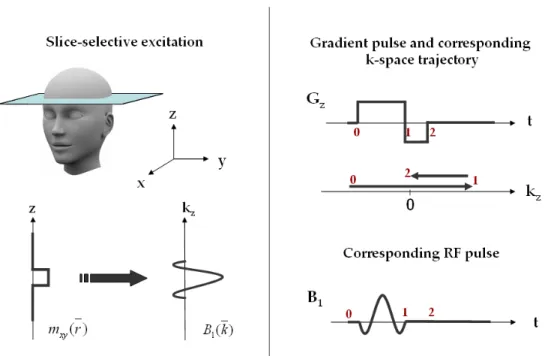
Figure 3: Slice‐selective excitation; left: target excitation and its Fourier transform, right: corresponding gradient and RF pulses.
According to the Fourier relation, to excite a slice we will need to create a sinc like RF pulse in k‐space (Figure 3, LHS). If we used the gradient pulse as specified on the top right of Figure 3, then the resulting k‐space can be found using Equation 3. This is also shown in Figure 3. During the time period 0 to 1, the k‐space trajectory travels from a negative to a positive value passing though the origin. If we play out a sinc pulse during this period then we would get the desired RF deposition in k‐space.
A more involved example would be the excitation of a two dimensional target profile in the x‐y plane (no variation in the z‐direction). For illustrative purposes the MIT logo is used as the target profile. Figure 4 shows the logo along with its Fourier transform. Note, in this excitation, the amount of excitation on the main part of “i” will be twice that of the other parts of the logo.
Figure 4: MIT logo target excitation profile and its transform
Figure 5: 2D excitation design; top: target’s Fourier transform and spiral k‐space trajectory, bottom: corresponding RF and gradient pulses, and the resulting excitation profile.
For the excitation design to work well, a suitable k‐space trajectory must be chosen such that it will cover the two dimensional k‐space sufficiently without under‐ sampling (i.e. taking account of aliasing). To achieve a short excitation period, the duration of the trajectory must be kept to a minimum. Hardware limitation on the
maximum achievable gradient amplitude G, and slew rate (
d G dt
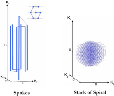
), translates to limitation on the velocity and acceleration of the k‐space trajectory (via Equation 3). Taking these constraints into account, a “spiral” k‐space trajectory is one choice for two dimensional excitations. Figure 5 shows the spiral trajectory and, the resulting RF and gradients waveforms. Also shown is the excitation profile produced by this design in a water phantom experiment using a Siemens 3T MRI system (22).The main intuition in designing k‐space trajectories is in trying to come up with a fast trajectory path that will sufficiently cover the high energy region and not cause aliasing, while still satisfying the slew and amplitude limitations of the gradient amplifiers. Since the overall shape of the high energy region depends on the target excitation pattern, a particular trajectory will not always be suitable for every excitation pattern. Figure 6 shows, two of the many possible three dimensional k‐space trajectories (22).
In this thesis, the spokes trajectory (22‐25) shown in Figure 6 will be used extensively for B1+ inhomogeneity mitigation. The aim of this design is to create sharp
slice‐selective excitation using sinc‐like excitation along kz, with some control of
modulating the in‐plane (x‐y) excitation profile to counter‐act the in‐plane B1+
inhomogeneity, via using amplitude and phase modulation of the different sinc “kz
spokes” that are place at various kx‐ky locations, to create an excitation pattern that is a
spatial inverse of the inhomogeneity. This trajectory choice is motivated by the need for relatively sharp slice profiles (i.e. large extent in kz) and relatively slowly‐varying in‐ plane mitigation patterns (i.e. smaller coverage in kx‐ky).
1.2.2 Parallel Transmission Theory
As previously mentioned, the technical limitation of multi‐dimensional, spatially selective excitation is in the rather long duration over which the RF and the gradient pulses need to be played out. Naturally, the pulse duration increases with the shape complexity of the volume of interest. RF and gradient pulses that obey practical amplitude and slew rate limitations (ultimately limited by physiological parameters, not hardware) and excite complex patterns are often too long for clinical application and are prone to system imperfection (12); and hence are not widely used. For example, slice‐ selective excitations that mitigate severe B1+ inhomogeneity via the use of spokes
trajectory can be very long because of the large number of kz spokes required on many
kx‐ky locations to sufficiently create an in‐plane excitation pattern that counteract the
severe inhomogeneity.
With the emergence of parallel transmission techniques, however, excitation pulses can be shortened, or equivalently, ’accelerated’ relative to the single‐channel implementations (8‐11). This results in the possibility of realizing more complex excitation patterns with practical pulse durations, which can be used in e.g. spatial modulation of the B1+ excitation profile to mitigate RF field inhomogeneity at high‐field (26‐28), and in creating high resolution image of a particular target region e.g. of a
suspected tumor (by selectively exciting only the target area, the signal acquisition phase of MRI can be modified to provide higher resolution image.
In describing parallel transmission, first an intuitive example is given to build insight into the technique. Following this, a more formal mathematical formulation is provided to allow for RF and gradient pulses design. The final part of this section will touch briefly on the important issues related to parallel transmission’s RF coil design, and how parallel transmission can help mitigate B1+ inhomogeneity.
An Intuitive Parallel Transmission Example
To explain parallel transmission, first the concept of B1+ sensitivity profile is described.
The B1+ sensitivity profile refers to the spatial variation of the RF field produced when a
current is applied to the coil. The profile will depend on shape and position of the coil. In the single‐channel transmission case, the RF coil is designed such that its sensitivity profile is uniform across space. Generally this is achieved via the use of a “birdcage” coil which is design to produce uniform field using the “uniform birdcage mode”.1 (Note:
the uniform birdcage mode’s RF field is not homogenous at high B0 field, hence the B1+
inhomogeneity problem).
In Parallel transmission, RF pulses on multiple independent RF coils are transmitted jointly to produce the desired excitation pattern. The B1+ sensitivity profiles
of these RF coils are design to be spatially varying and different. The different in the sensitivity profile among the coils is the key to shortening the excitation duration. To illustrate this, a simple idealized example is given in Figure 7 and Figure 8, where two RF coils are used to reduce the duration of a 2D excitation. In this example, the target excitation pattern will be a circle at the center of x‐y origin, and a 2D k‐space trajectory, termed echo‐planer (EP), will be used. As shown in Figure 7, excitation acceleration will be achieved by using a k‐space trajectory with sparser sampling (2x) along kx axis;
resulting in a duration reduction of two for both gradient and RF pulses. In standard
1
The uniform birdcage mode will be explained in detail in the background section titled Parallel Transmission’s RF Coil Design and Mode Compression, see pp. 35-37.
single‐channel design, due to under‐sampling, this accelerated EP trajectory will result in excitation warp‐around into the field of view1 (aliasing) along the x‐axis as shown in
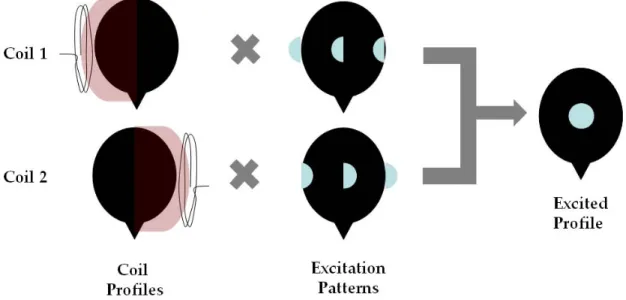
Figure 7. For parallel transmission, the variation in the sensitivity profiles among the RF coils is used to get around this problem. To demonstrate this, two transmission coils with idealized sensitivity profiles are used, where profile of coil 1 is uniform across the left half of the head and profile of coil 2 is uniform across the right, with no overlapping in area between (Figure 8). With careful design of excitation pattern for each of the coil, the desired excitation pattern can be achieved using the accelerated EP trajectory. This is shown in Figure 8. Note: the excitation produced by each coil is the product of the designed excitation pattern and the coil sensitivity, and the total excitation is the sum of the excitations produced by all the transmission coils. Figure 7: Cylindrical target excitation and the results of single‐channel Echo Planer excitation with 2X acceleration leading to aliasing/wrap‐around effect
1
Figure 8: Cylindrical excitation (2X) via parallel transmission of two orthogonal RF coils resulting in no aliasing/wrap‐around effect
This example gives an intuitive picture on how parallel transmission works. However, in reality the coil sensitivity profiles are not as well behaved, or as orthogonal, as the example assumes. They generally exhibit rapid spatial variation and are significantly overlapped. As a result the RF design process is more complex. The mathematical formulation below provides an outline of the actual design method used in parallel transmission.
Mathematical Formulation
Various methods have been proposed for parallel RF excitation design based on the small tip angle approximation presented earlier via Equation 2 and Equation 3. The use of this linear approximation greatly reduces computation and provides attractive intuition about design tradeoffs since the RF design problem is reduced to a linear, and in fact a Fourier system. In the method presented by Katscher et al. (8), the system of linear equations are solved in the excitation Fourier space, k‐space. On the other hand, the scheme developed by Zhu (9) was formulated in the spatial domain with the
assumption of an echo‐planar k‐space trajectory. Another method proposed by Griswold et al. (10) draws on the “GRAPPA” technique (29) used in accelerating data acquisition with receive arrays, and is solved in the k‐space domain. Finally, Grissom et al. (11) formulated the design as a direct discretization of the parallel small tip angle equation in space and time. The small‐tip‐angle work in this thesis starts with Grissom’s formulation as the baseline, where the parallel small‐tip excitation approximation with R coils is written as Equation 4 ( ) 0 1 1, 0
( )
C( )
T( )
i r k t xy c c cm
r
=
i m
γ
∑
=S r
∫
b
t e
⋅dt
This is a direct extension of Equation 2, where in this case the resulting magnetization is the sum of the magnetization produced from each of the coils. Furthermore, an extra term appears in this equation due to the coils’ B1+ sensitivity
profiles, S rc( ). In the single coil case, the profile was assumed to be uniform in space,
and hence its exclusion from Equation 2.
After discretization of space and time, this expression can be written as a matrix equation,m= Ab, where the A‐matrix incorporates the B1+ coil profiles modulated by the
Fourier kernel due to the k‐space traversal, m is the target profile in space, and b contains the RF waveforms. With this formulation, the RF pulses can be designed by solving the following optimization problem by the conventional Least Squares (LS) algorithm: Equation 5 2
arg min{
b( )}
wb
=
Ab
−
m
+
R b
Here, the optimization is performed over the Region of Interest implied by a weighting, w, andR b
( )
denotes a regularization term that may be use to control integrated and peak RF power. Generally the Tikhonov regularization (R b
( )
=
β
b b
'
) is used, and the minimization problem can be solved efficiently using conjugate‐gradient (CG) methods.Parallel Transmission’s RF Coil Design and Mode Compression
One of the major requirements in parallel excitation is to have good orthogonality between RF coils transmission profiles to allow good acceleration performance. This is not easy to achieve due to the coupling effect between the RF coils. Generally, parallel transmission RF coil arrays are built around a cylindrical ring with a number of local coil elements placed adjacent to each other, with some means of decoupling them. Figure 9 shows some of the coil arrays that were used in this work. The loop array on the left (a) is decoupled via overlapping the coil elements, and the stripline arrays in (b) and (c) are decoupled via capacitive means (30,31). Figure 9: RF coil arrays employed in this work: (a) eight‐channel loop coil array at 3T, (b) eight‐ channel stripline array at 7T, (c) sixteen‐channel stripline array at 7T.
With more RF coil elements, higher transmission acceleration can be achieved. Nonetheless, as more elements are built into a coil array, the coil profiles of these elements become less orthogonal, resulting in a smaller achievable acceleration gain. Furthermore, for each additional transmission channel, an extra set of RF amplifier hardware is required. These hardware components are expensive and pose a practical limit on the number of transmission channels that can be used. To partially overcome this limitation, the idea of “mode compression” is employed, whereby orthogonal “modes” instead of the individual coil elements of the array are used for transmission to significantly reduce the number of transmission channels required (31). To understand this concept, first an explanation of a “mode” will be given, followed by an explanation on how it could be use to reduce the number of transmission channels.
The transmission profiles of the coil elements in an array can be thought of as a basis set which are not very orthogonal. Therefore, one should be able to apply a basis transformation to create an orthogonal basis set with a reduced number of bases. “Modes” of a coil array can be thought of as an orthogonal basis set. Many different types of modes exist. By constructing the coil array using the principle of degenerate birdcage coil design (31), the “birdcage” modes can be created from the array. To create each of these birdcage modes, RF transmission with the same amplitude but different phase are sent to the coil elements. For an N‐channels array, the Mth mode is created by
driving the coil elements C1, C2, C3,…., CN with the same amplitude but with a phase
relationship of
0,
M
2
,
M
4
,....,
M N
(
1)
2
N
N
N
π
π
π
−
. The profile of the first mode (M=1)generated by the degenerated birdcage coil is the same as the profile of the standard single channel birdcage coil that was previously described. In the standard birdcage coil, the coil elements are linked and are designed to have a mode‐1 phase relationship when RF is transmitted into the single input channel of the coil. The profile produced by this mode is uniform1 and is referred to as “uniform birdcage mode”. The higher order
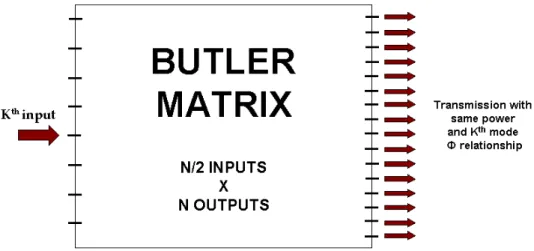
modes have strong spatial variation and are not used in conventional imaging. For an N‐ channel coil, there are N possible birdcage modes; half of which do not provide significant excitation due to their counter‐rotation property (31). Nonetheless, the N/2 remaining modes provide useful transmissions and have a high degree of orthogonality. The mode compression idea is based on “butler matrix” hardware (31), which can generate the N/2 useful modes using N/2 instead of N sets of RF amplifier. Given the availability of N/2 RF amplifiers, the N/2 highly decoupled mode profiles generated by an N‐channel array is much preferred over the profiles produced by an N/2‐channel coil array driven directly though the RF amplifiers. When in use, the butler matrix hardware is placed between the coil and the RF amplifiers. Figure 10 shows a diagram of the butler matrix with N/2 inputs from the amplifiers and N outputs to the coil array’s elements. The butler matrix splits the input power from the kth amplifier and feeds it
1
equally into each of the N output channels with appropriate phase shifts to generate the kth birdcage mode of the array. In this work, an 8x16 butler matrix hardware (31) is used
to drive the 16‐channel stripline coil array shown in Figure 9c, on our 8‐channel transmission system at 7T.
Figure 10: Diagram of the Butler matrix with N/2 inputs from the RF amplifiers and N outputs to the transmission coil elements. The power transmitted by the kth amplifier is split into equal parts and feed
to the output with appropriate phase shifts to generate the kth birdcage mode.
As a side note, RF coil arrays are also widely employed for signal reception during the data acquisition phase of MRI. In the single channel reception case, signal received by the coil elements are usually designed to have a mode‐1 phase relationship resulting in “uniform birdcage” reception. In multi‐channel reception, parallel reception techniques (29,32,33), which were develop prior to parallel transmission, are used to accelerate data encoding. However, unlike parallel transmission, in parallel reception the receive hardware are relatively inexpensive (pre‐amps instead of power amps), allowing for a large number of coil elements to be used, with a recently achieved coil array count of 128 (34,35).
B
1+mitigation via Parallel Transmission
As previously mentioned, the uniform birdcage RF field of a coil array is spatially inhomogeneous at high B0 field. At high field strength, Larmor frequency