HAL Id: hal-01263994
https://hal.inria.fr/hal-01263994
Submitted on 28 Jan 2016
HAL is a multi-disciplinary open access
archive for the deposit and dissemination of
sci-entific research documents, whether they are
pub-lished or not. The documents may come from
teaching and research institutions in France or
abroad, or from public or private research centers.
L’archive ouverte pluridisciplinaire HAL, est
destinée au dépôt et à la diffusion de documents
scientifiques de niveau recherche, publiés ou non,
émanant des établissements d’enseignement et de
recherche français ou étrangers, des laboratoires
publics ou privés.
Partitioned Time-triggered Real-time Implementation *
Thomas Carle, Dumitru Potop-Butucaru, Yves Sorel, David Lesens
To cite this version:
Thomas Carle, Dumitru Potop-Butucaru, Yves Sorel, David Lesens. From Dataflow Specification
to Multiprocessor Partitioned Time-triggered Real-time Implementation *. Leibniz Transactions on
Embedded Systems, European Design and Automation Association (EDAA) EMbedded Systems
Special Interest Group (EMSIG) and Schloss Dagstuhl – Leibniz-Zentrum für Informatik GmbH,
Dagstuhl Publishing., 2015, �10.4230/LITES-v002-i002-a001�. �hal-01263994�
Partitioned Time-triggered Real-time
Implementation
∗
Thomas Carle
1, Dumitru Potop-Butucaru
2, Yves Sorel
3, and
David Lesens
41 Brown University
247 Browen Street, Providence, Rhode Island 02906, USA http://orcid.org/0000-0002-1411-1030
[email protected] 2 INRIA Paris-Rocquencourt
Domaine de Voluceau, Rocquencourt – B.P. 105, 78153 Le Chesnay, France http://orcid.org/0000-0003-3672-6156
[email protected] 3 INRIA Paris-Rocquencourt
Domaine de Voluceau, Rocquencourt – B.P. 105, 78153 Le Chesnay, France [email protected]
4 Airbus Defence & Space
Route de Verneuil, 78133 Les Mureaux, France http://orcid.org/0000-0002-3452-9960
Abstract
Our objective is to facilitate the development of complex time-triggered systems by automating the allocation and scheduling steps. We show that full automation is possible while taking into account the elements of complexity needed by a complex em-bedded control system. More precisely, we consider deterministic functional specifications provided (as often in an industrial setting) by means of syn-chronous data-flow models with multiple modes and multiple relative periods. We first extend this functional model with an original real-time characterization that takes advantage of our time-triggered framework to provide a simpler repres-entation of complex end-to-end flow requirements. We also extend our specifications with additional non-functional properties specifying partitioning, al-location, and preemptability constraints. Then, we
provide novel algorithms for the off-line schedul-ing of these extended specifications onto parti-tioned time-triggered architectures à la ARINC 653. The main originality of our work is that it takes into account at the same time multiple com-plexity elements: various types of non-functional properties (real-time, partitioning, allocation, pree-mptability) and functional specifications with con-ditional execution and multiple modes. Allocation of time slots/windows to partitions can be fully or partially provided, or synthesized by our tool. Our algorithms allow the automatic allocation and scheduling onto multi-processor (distributed) sys-tems with a global time base, taking into account communication costs. We demonstrate our tech-nique on a model of space flight software system with strong real-time determinism requirements.
2012 ACM Subject Classification Computer systems organization Real-time systems
Keywords and phrases Time-triggered, off-line real-time scheduling, temporal partitioning
Digital Object Identifier 10.4230/LITES-v002-i002-a001
Received 2013-10-01Accepted 2015-07-22Published 2015-10-01
1
Introduction
This paper addresses the implementation of embedded control systems with strong functional and temporal determinism requirements. The development of these systems is usually based on model-driven approaches using high-level formalisms for the specification of functionality (Simulink, Scade[11]) and/or real-time system architecture and non-functional requirements (AADL [18], UML/Marte [34]).
The temporal determinism requirement also means that the implementation is likely to use time-triggered architectures and execution mechanisms defined in well-established standards such
as TTA, FlexRay [44], ARINC 653 [3], or AUTOSAR [5].
The time-triggered paradigm describes sampling-based systems (as opposed to event-driven ones) [28] where sampling and execution are performed at predefined points in time. The offline computation of these points under non-functional constraints of various types (real-time, temporal isolation of different criticality sub-systems, resource allocation) often complicates system development, when compared to classical event-driven systems. In return for the increased design cost, system validation and qualification are largely simplified, which explains the early adoption of time-triggered techniques in the development of safety- and mission-critical real-time systems.
1.1
Contribution
The objective and contribution of this paper is to facilitate the development of time-triggered systems by automating the allocation and scheduling steps for significant classes of functional specifications, target time-triggered architectures, and non-functional requirements. On the application side, we consider general dataflow synchronous specifications with conditional execution, multiple execution modes, and multiple relative periods. Explicitly taking into account conditional execution and execution modes during scheduling is a key point of our approach, because the offline computation of triggering dates limits flexibility at runtime. For instance, taking into account conditional execution and modes allows for better use of system resources (efficiency) and a simple modeling of reconfigurations.
On the architecture side, we consider multiprocessor distributed architectures, taking into account communication costs during automatic allocation and scheduling.
In the non-functional domain, we consider real-time, partitioning, preemptability, and allocation constraints. By partitioning we mean here the temporal partitioning specific to TTA, FlexRay (the static segment), and ARINC 653, which allows the static allocation of CPU or bus time slots, on a periodic basis, to various parts (known as partitions) of the application. Also known as static time division multiplexing (TDM) scheduling, partitioning further enhances the temporal determinism of a system.
The main originality of our paper is to consider all these aspects together, in an integrated fashion, thus allowing the automatic implementation for complex real-life applications. Other originality points concern the specification of real-time properties, which we adapted to our time-triggered framework, and the handling of partitioning information. In the specification of real-time properties, the use of deadlines that are longer than the periods naturally arises. It allows a more natural real-time specification, improved schedulability, and less context changes between partitions (which are notoriously expensive). Regarding the partitioning information, allocation of time slots/windows to partitions can be fully or partially provided, or synthesized by our tool.
Single−period acyclic dependent
task system table
Offline multiprocessor scheduling (section 6) Scheduling table (section 6.1) Optimization (section 7) Optimized scheduling Removal of delayed dependencies (section 5) Single−period dependent task system Hyperperiod expansion (section 4.1.2) Multiperiodic dependent task system (section 4.1.2) (section 4.1.3) modeling Case study (sec. 3, 4.1.1, 4.2)
Figure 1 The proposed implementation flow.
1.2
The Application
We apply our technique on a model of spacecraft embedded control system. Spacecrafts are subject to very strict real-time requirements. The unavailability of the avionics system (and thus of the software) of a space launcher during a few milliseconds during the atmospheric phase may indeed lead to the destruction of the launcher. From a spacecraft system point of view, the latencies are defined between acquisitions of measurement by a sensor to sending of commands by an actuator. Meanwhile, the commands are established by a set of control algorithms (Guidance, Navigation and Control or GNC).
Traditionally, the GNC algorithms are implemented on a dedicated processor using a classical multi-tasking approach. But today, the increase of computational power provided by space processors allows suppressing this dedicated processor and distributing the GNC algorithms on the processors controlling either the sensors or the actuators. For future spacecraft (space launchers or space transportation vehicles), the navigation algorithm could for instance run on the processor controlling the gyroscope, while the control algorithm could run on the processor controlling the thruster. The suppression of the dedicated processor allows power and mass saving.
But the sharing of one processor by several pieces of software of different Design Assurance Levels (e.g. gyroscope control and navigaton) requires the use of an operating system ensuring the Time and Space Partitioning (or TSP) between these pieces of software. Such operating systems, like ARINC 653 [3], feature a hierarchic 2-level scheduler where the top-level one is of static time-triggered (TDM) type. Furthermore, for predictability issues, the processors of the distributed implementation platform share a common time base. This means that the execution platform offers the possibility of a globally time-triggered implementation. We therefore aim for distributed implementations that are time-triggered at all levels, which improves system predictability and allows the computation of tighter worst-case bounds on end-to-end latencies.
The scheduling problem we consider is therefore as follows: End-to-end latencies are defined at spacecraft system level, along with the offsets of sensing and actuation operations. Also provided are safe worst case execution time (WCET) estimations associated to each task on each processor on which they can be executed. What must be computed is the time-triggered schedule of the system, including the activation times of each partition and each task, and the bus frame.
1.3
Proposed Implementation Flow and Paper Outline.
The remainder of the paper is organized as follows. Section 2 reviews related work. Section 3 presents our target execution platforms. It spends significant space on the careful definition of time-triggered and partitioned systems. Sections 4 to 7 define the proposed implementation flow for time-triggered systems, whose global structure is depicted in Figure 1. These sections also present experimental results. Section 8 concludes.
The two types of boxes in Figure 1 (dashed and solid) reflect the dual nature of our paper, which contains not only work on the definition of new scheduling algorithms, but also on integrating these algorithms into a larger implementation flow. First of all, our paper provides the full formal specification of an off-line scheduling problem for single-period dependent task systems with complex non-functional requirements. We also provide optimized scheduling algorithms for solving this problem. The task model taken as input by these algorithms is that of Definition 2, augmented with the formal definitions of Section 3 (architecture, partitions, windows, MTF) and the non-functional property definitions of Section 4.2 (release dates, deadlines). The output of the algorithms is a scheduling table, formally defined in Section 6.1. These formalisms and algorithms, whose presentation takes most of the paper, are represented with solid boxes in Figure 1.
The remaining (dashed) boxes represent implementation steps that are needed to ensure the practical applicability of our work, but which either bring no scientific contribution (e.g. hyper-period expansion) or which concern the initial modeling steps, which are not fully automatable. This is why we only dedicate them two subsections and use an example-driven presentation. We also use examples to explain how the formal constructs of the task model can be used to model various non-functional requirements arising in practical system design. For instance, in Section 4.2.1.4 we use our case study to show how release dates and deadlines can be used to model one type of architecture-related constraints (related to the size of the input buffers).
2
Related Work
The main originality of our work is to define a complex task model allowing the specification of all the functional and non-functional aspects needed for the efficient implementation of our case study. Of course, prior work already considers all these functional and non-functional aspects, but either in isolation (one aspect at a time), or through combinations that do not cover our modeling needs. Our contributions are the non-trivial combination of these aspects in a coherent formal model and the definition of synthesis algorithms able to build a running real-time implementation.
Previous work by Henzinger et al. [26, 25], Forget et al. [37], Marouf et al. [33], and Alras et al. [2] on the implementation of multi-periodic synchronous programs and the work by Blazewicz [7] and Chetto et al. [12] on the scheduling of dependent task systems have been important sources of inspiration. By comparison, our paper provides a general treatment of ARINC 653-like partitioning and of conditional execution, and a novel use of deadlines longer than periods to allow faithful real-time specification.
The work of Caspi et al. [11] addresses the multiprocessor scheduling of synchronous programs under bus partitioning constraints. By comparison, our work takes into account conditional execution and execution modes, allows preemptive scheduling, and allows automatic allocation of computations and communications. Taking advantage of the time-triggered execution context, our approach also relies on fixed deadlines (as opposed to relative ones), which facilitates the definition of fast mapping heuristics.
Another line of work on the scheduling of dependent tasks is represented by the works of Pop et al. [38] and Wei Zheng et al. [47]. In both cases, the input of the technique is a DAG, whereas our functional specifications allow the use of delayed dependencies between successive iterations of the DAG. Other differences are that the technique [47] does not take into account ARINC 653-like partitioning or conditional execution, and the technique of [38] does not allow the specification of complex end-to-end latency constraints. Fohler [20] does consider conditional control, but does so in a mono-processor, non-partitioned, non-preemptive context.
The off-line (pipelined) scheduling of tasks with deadlines longer than the periods has been previously considered (among others) by Fohler and Ramamritham [21], but this work does not
consider, as we do, partitioning constraints and the use of execution conditions to improve resource allocation. This is also our originality with respect to other classical work on static scheduling of periodic systems [42].
Compared to previous work by Isovic and Fohler [27] on real-time scheduling for predictable, yet flexible real-time systems, our approach does not directly cover the issue of sporadic tasks, but allows a more flexible treatment of periodic (time-triggered) tasks. Based on a different representation of real-time characteristics and on a very general handling of execution conditions, we allow for better flexibility inside the fully predictable domain.
From an implementation-oriented perspective, Giotto [25, 26], ΨC [32], and Prelude [37, 41] make the choice of mixing a globally time-triggered execution mechanism with on-line priority-driven scheduling algorithms such as RM or EDF. By comparison, we made the choice of taking all scheduling decisions off-line. Doing this complicates the implementation process, but imposes a form of temporal isolation between the tasks which reduces the number of possible execution traces and increases timing precision (as the scheduling of one task no longer depends on the run-time duration of the others). In turn, this facilitates verification and validation. Furthermore, a fully off-line scheduling approach such as ours has the potential of improving worst-case performance guarantees by taking better decisions than a RM/EDF scheduler which follows an as-soon-as-possible (ASAP) scheduling paradigm. For instance, the transformations of Section 7 reduce the number of notoriously expensive partition changes by using a scheduling technique that is not ASAP. These partition changes are not taken into account in the optimality results concerning the EDF scheduling of Prelude [37].
Compared to classical work on the on-line real-time scheduling of tasks with execution modes (cf. [6]), our off-line scheduling approach comes with precise control of timing, causalities, and the correlation (exclusion relations) between multiple test conditions of an application. It is therefore more interesting for us to use a task model that explicitly represents execution conditions. We can then use table-based scheduling algorithms that precisely determine when the same resource can be allocated at the same time to two tasks because they are never both executed in a given execution cycle.
The use of execution conditions to allow efficient resource allocation is also the main difference between our work and the classical results of Xu [46]. Indeed, the exclusion relation defined by Xu does not model conditional execution, but resource access conflicts, thus being fundamentally different from the exclusion relation we define in Section 4. Our technique also allows the use of execution platforms with non-negligible communication costs and multiple processor types, as well as the use of preemptive tasks (unlike in Xu’s paper).
The off-line scheduling on partitioned ARINC 653 platforms has been previously considered, for instance by Al Sheikh et al. [45] and by Brocal et al. in Xoncrete [8]. The first approach only considers systems with one task per partition, whereas our work considers the general case of multiple tasks per partition. The second approach (Xoncrete) allows multiple tasks per partition, but does not seem interested in having a functionally deterministic specification and preserving its semantics during scheduling (as we do). For instance, its input formalism does not specify periods, but ranges of acceptable periods, and the first implementation step adjusts these periods to reduce their lowest common multiple (thus changing the semantics1). Other differences are that our approach can take into account conditional execution and execution modes, and that we allow scheduling onto multi-processors, whereas Xoncrete does not.
More generally, our work is related to work on the scheduling for precision-timed architectures (e.g. [17]). Our originality is to consider complex non-functional constraints. The work on the
PharOS technology [32] also targets dependable time-triggered system implementation, but with two main differences. First, we follow a classical ARINC 653-like approach to temporal partitioning. Second, we take all scheduling decisions off-line. This constrains the system but reduces the scheduling effort needed from the OS, and improves predictability.
References on time-triggered and partitioned systems, as well as scheduling of synchronous specifications will be provided in the following sections.
3
Architecture Model
In this paper, we consider both single-processor architectures and bus-based multi-processor architectures with a globally time-triggered execution model and with strong temporal partitioning mechanisms. This class of architectures covers the needs of the considered case study, but also covers platforms based on the ARINC 653, TTA, and FlexRay (the static segment) standards.
Formally, for the scope of this paper, an architecture is a pair Arch = (B(Arch),
Procs(Arch)) formed of a broadcast message-passing bus B(Arch) connecting a set of processors Procs(Arch) = {P1, . . . , Pn} for some n ≥ 1. We assume that the bus does not lose, create,
corrupt, duplicate or change the order of messages it transmits. Previous work by Girault et al. [22] (among others) can be used to extend this simple model (and the algorithms of this paper) to deal with fault-tolerant architectures with multiple communication lines and more complex interconnect topologies. The architecture supports a time-triggered, partitioned execution model detailed below.
3.1
Time-triggered Systems
In this section we define the notion of time-triggered system used in this paper. It roughly corresponds to the definition given by Kopetz [28], and is a sub-case of the definition given by Henzinger and Kirsch [26]. We shall introduce its elements progressively, explaining what the consequences are in practice.
3.1.1
General Definition
By time-triggered systems we understand systems satisfying the following 3 properties:
TT1 A system-wide time reference exists. We shall refer to this time reference as the global clock.2 All timers in the system use the global clock as a time base.
TT2 The execution duration of code driven by interrupts other than the timers (e.g. interrupt-driven driver code) is negligible. In other words, for timing analysis purposes, code execution is only triggered by timers synchronized on the global clock.
TT3 System inputs are only read/sampled at timer triggering points.
This definition places no constraints on the sequential code triggered by timers. In particular: Classical sequential control flow structures such as sequence or conditional execution are permitted, allowing the representation of modes and mode changes.
Timers are allowed to preempt the execution of previously-started code.
This definition of time-triggered systems is fairly general. It covers single-processor systems that can be represented with time-triggered e-code programs, as they are defined by Henzinger and
2 For single-processor systems the global clock can be the CPU clock itself. For distributed multiprocessor systems, we assume it is provided by a platform such as TTA [29] or by a clock synchronization technique such as the one of Potop et al. [39].
Kirsch [26]. It also covers multiprocessor extensions of this model, as defined by Fischmeister et al. [19] and used by Potop et al. [39]. In particular, our model covers time-triggered communication infrastructures such as TTA and FlexRay (static and dynamic segments) [29, 44], the periodic schedule tables of AUTOSAR OS [5], as well as systems following a multi-processor periodic scheduling model without jitter and drift.3 It also covers the execution mechanisms of the avionics
ARINC 653 standard [3] provided that interrupt-driven data acquisitions, which are confined to the ARINC 653 kernel, are presented to the application software in a time-triggered fashion satisfying property TT3. One way of ensuring that TT3 holds is presented in [35], and to our knowledge, this constraint is satisfied in all industrial settings.
3.1.2
Model Restriction
The major advantage of time-triggered systems, as defined above, is that they have the property of repeatable timing [16]. Repeatable timing means that for any two input sequences that are identical in the large-grain timing scale determined by the timers of a program, the behaviors of the program, including timing aspects, are identical. Of course, this ideal property must be amended to take into account the fact that the global clock may not be very accurate or that interrupt-driven driver code does take time and influences the execution of time-triggered code. In practice, however, repeatability can be ensured with good precision. Repeatability is extremely valuable in practice because it largely simplifies debugging and testing of real-time programs. A time-triggered platform also insulates the developer from most problems stemming from interrupt asynchrony and low-level timing aspects.
However, the applications we consider have even stronger timing requirements, and must satisfy a property known as timing predictability [16]. Timing predictability means that formal timing guarantees covering all possible executions of the system should be computed off-line by means of (static) analysis. The general time-triggered model defined above remains too complex to allow the analysis of real-life systems. To facilitate analysis, this model is usually restricted and used in conjunction with WCET analysis of the sequential code fragments.
In this paper we consider a restriction of the general definition provided above. In this restriction, timers are triggered following a fixed pattern which is repeated periodically in time. Following the convention of ARINC 653, we call this period the major time frame (MTF). The timer triggering pattern is provided under the form of a set of fixed offsets 0 ≤ t1< t2< . . . < tm< MTF defined
with respect to the start of each MTF period. Note that the code triggered at each offset may still involve complex control, such as conditional execution or preemption.
This restriction corresponds to the classical definition of time-triggered systems by Kopetz [28, 29]. It covers our target platform, TTA, FlexRay (the static segment), and AUTOSAR OS (the periodic schedule tables). At the same time, it does not fully cover ARINC 653. As defined by this standard, partition scheduling is time-triggered in the sense of Kopetz. However, the scheduling of tasks inside partitions is not, because periodic processes can be started (in normal mode) with a release date equal to the current time (not a predefined date). To fit inside Kopetz’s model, an ARINC 653 system should not allow the start of periodic processes after system initialization, i.e. in normal mode.
3.2
Temporal Partitioning
Our target architectures follow a strong temporal partitioning paradigm similar to that of ARINC 653.4 In this paradigm, both system software and platform resources are statically divided among a
finite set of partitions Part = {part1, . . . , partk}. Intuitively, a partition comprises both a software
application of the system and the execution and communication resources allocated to it. The aim of this static partitioning is to limit the functional and temporal influence of one partition on another. Partitions can communicate and synchronize only through a set of explictly-specified inter-partition channels.
We are mainly concerned in this paper with the execution resource represented by the processors. To eliminate timing interference between partitions running on a processor, the static partitioning of the processor time is done using a static time division multiplexing (TDM) mechanism. In our case, the static TDM mechanism is built on top of the time-triggered model of the previous section. It is implemented by partitioning, separately for each processor Pi, the MTF defined
above into a finite set of non-overlapping windows Wi= {wi1, . . . , w ki
i }. Each window w j i has a
fixed start offset twji, a duration dwji, and it is either allocated to a single partition partwji, or left unused. Unused windows are called spares and identified by partwji = spare.
Software belonging to partition parti can only be executed during windows belonging to parti. Unfinished partition code will be preempted at window end, to be resumed at the next window of the partition. There is an implicit assumption that the scheduling of operations inside the MTF will ensure that non-preemptive operations will not cross window end points.
For the scheduling algorithms of Section 6, the partitioning of the MTF into windows can be either an input or an output. More precisely, all, none, or part of the windows can be provided as input to the scheduling algorithms.
3.3
Example
To present the type of partitioned time-triggered system we synthesize and the underlying execution mechanisms, we rely on the example of Figure 2. This example will gradually introduce conditional execution and deterministic mode changes, pre-computed preemptions, and the pipelined execution of operations (operations that start in one MTF and complete in the next), which poses significant problems, especially when combined with conditional execution. The formal definitions supporting the intuitive presentation of the example will be provided in the following sections.
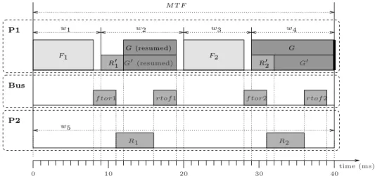
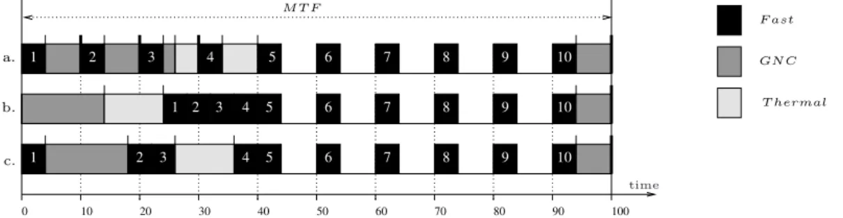
Our system has two processors, denoted P1 and P2, which are connected via a bus. As explained above, execution is periodic. Our figure provides the execution pattern for one period, under the form of a scheduling table. A full execution of the system is obtained by indefinitely repeating this pattern. In our case, the length of the scheduling table, which gives the MTF (global period) of the system is 40 milliseconds (ms).
The scheduling table defines the start dates of all the operations that can be executed during one MTF, be them computations or communications. For operations that can be preempted, it also defines all the dates where they are preempted and resumed (all these dates are pre-computed off-line). Finally, our table also defines the worst-case end dates of the operations. All dates are defined in the time reference of the global clock provided by the time-triggered platform. In our example, this clock (pictured at the bottom of the figure) has a precision of 1 ms. For instance, operation F1
starts in each MTF at date 0 and ends (in the worst case) at date 8. Synchronization of operations with respect to the global clock also ensures the correct synchronization between operations. For
w1 w2 w3 w4 P1 F1 F2 Bus P2 0 10 20 30 40 time (ms) R1 R2 G R′2 G′ R′1 G (resumed) G′ (resumed) w5 M T F
f tor1 rtof 1 f tor2 rtof 2
Figure 2 An example of time-triggered partitioned system. In this example only processor P1 requires
partitioning.
instance, F1 ending before date 8 allows the synchronization with the communication ftor1 which
transmits a value from F1to R1.
To comply with Kopetz’ time-triggered model, the start/preempt/resume dates of all operations are computed off-line. For instance, on processor P1 operations can only start at dates 0, 9, 20, 29, and 32. However, code triggered at each offset may involve complex control such as conditional execution or preemption. Our example features both. Conditional execution is used here to represent execution modes. There are 2 modes. In mode1 are executed F1, F2, G, R1, R2 and the
bus communications. The other mode, named mode2, is meant to be activated when processor P 2 is removed from the system due to a hardware reconfiguration. In this mode, operations F1and F2remain unchanged, but the other are replaced with the lower-duration counterparts G0, R10,
and R20 (and no communication operations).
In our example, mode changes occur at the beginning of the MTF. Only operations belonging to the currently-active mode can be started during the MTF. Operations of different modes can be scheduled on the same processor at the same dates, as is the case for G and G0 and G and R20. This form of double reservation is forbidden if the operations belong to the same mode because our resources (processors and buses) are sequential.
Preemption is needed in the scheduling of long tasks and in dealing with partitioning. In our example, we assumed that the computation operations are divided in 2 partitions: part1 contains F1 and F2, and part2 all the other operations. During each MTF, the processor time of P1 is
statically divided in 4 windows. Windows w1 and w3 are allocated to part1, and windows w2 and w4are allocated to part2. To simplify the presentation of the algorithms we assume in this paper
that bus time is not partitioned. Processor P2 only executes operations of part2, so that its MTF contains one window w5 spanning over the entire MTF.
Window w4 starts at date 29 and ends at date 40. Operation G starts at date 29, but its
worst-case duration is 18 ms, longer than the 11 ms of w4. Since window w1 belongs to another
partition, operation G must be pre-empted at the end of w4, and it can be resumed at date 12
(within w2) in the next MTF. Our scheduling table therefore contains a pre-computed preemption
(represented with a thick black bar at the end of G in w4), and the execution time of G is divided
between 2 windows. Similarly, the execution of G0 is divided in two by a precomputed preemption. An important hypothesis in our work is that the scheduling table specifies not only the start date of an operation, but also the dates where an operation can resume after a pre-computed
preemption. For instance, operations G and G0 resume at date 12, not at date 9. This hypothesis facilitates scheduling. In time-triggered operating systems such as ARINC 653, where only start dates are specified, this hypothesis can be easily implemented by using simple manipulations of task priorities.5
Another important hypothesis we make is that once an operation is started, it must be completed. In other words, it can be preempted and resumed, but it cannot be aborted. This hypothesis is key in ensuring the predictability and determinism of our systems. Intuitively, an operation can change the state of sensors, actuators, or internal variables, and it is difficult to determine the system state after an abortion operation.
But the absence of abortion requires much care in dealing with conditional execution and execution mode changes. Assume, for instance, that operation G is started during one MTF, and that the mode changes from mode1 to mode2 at the end of that MTF. Then, the scheduling of the next MTF must allow G to resume and complete while ensuring that the operations of mode2 can be started. This explains why R01 and the resumed part of G cannot be scheduled at the same date, even though G and R01belong to different modes.
4
Task Model
Following classical industrial design practices, the specification of our scheduling problem is formed of a functional specification and a set of non-functional properties. Represented in an abstract fashion, these two components form what is classically known as a task model which allows the definition of our scheduling algorithms.
4.1
Functional Specification
Our scheduling technique works on deterministic functional specifications of dataflow synchronous type,6 such as those written in Scade/Lustre [11]. These formalisms, which are common in the design of safety-critical embedded control systems, allow the representation of dependent task systems featuring multiple execution modes, conditional execution, and multiple relative periods.
However, a full presentation of all the details of our formalism would only complicate the presentation of this paper. Instead, we define here a task model containing just the formal elements needed to define our scheduling algorithms, and then explain using intuitive examples how an abstract task system is obtained from a data-flow synchronous specification. The full formal definition of the synchronous formalism used by our tool and of its relation with other formalisms used in embedded systems design and real-time scheduling is provided in [9].
4.1.1
Single-period Dependent Task Systems
We define our task model in two steps. The first one covers systems with a single execution mode:
IDefinition 1 (Non-conditioned dependent task system). A non-conditioned dependent task system is a directed graph defined as a triple D = (TD, AD, ∆D). Here, TD is the finite set of tasks.
The finite set AD contains dependencies of the form a = (srca, dsta, typea), where srca, dsta∈ TD
5 By using helper tasks that are executed at the time triggering points, and which raise or lower the priority of the other tasks to ensure that the greatest priority belongs to the one that must be executed (started or resumed) in the following time slot.
6 Dataflow synchronous formalisms should not be confused with Lee and Messerschmitt’s Synchronous Data Flow (SDF) [30] and derived models. For instance, data-dependent conditional execution cannot be faithfully represented in SDF.
are the source, respectively the destination task of a, and typea the type of the data messages
transmitted from the source to the destination (identified by a name).7 The directed graph
determined by AD must be acyclic. The finite set ∆D contains delayed dependencies of the
form δ = (srcδ, dstδ, typeδ, depthδ), where srcδ, dstδ, typeδ have the same meaning as for regular
dependencies and depthδ is a strictly positive integer called the depth of the dependency8.
Non-conditioned dependent task systems have a cyclic execution model. At each execution cycle of the task system, each of the tasks is executed exactly once. We denote with tn the instance of task t ∈ TD for cycle n. The execution of the tasks inside a cycle is partially ordered by the
dependencies of AD. If a ∈ AD then the execution of srcan must be finished before the start of
dstan, for all n. Note that dependency types are explicitly defined, allowing us to manipulate
communication mapping.
The dependencies of ∆D impose an order between tasks of successive execution cycles. If
δ ∈ ∆D then the execution of srcδn must complete before the start of dstδn+depthδ, for all n.
We make the assumption that a task has no state unless it is explicitly modeled through a delayed arc. This assumption is a semantically sound way of providing more flexibility to the scheduler. Indeed, assuming by default that all tasks have an internal state (as classical task models do) implies that two instances of a task can never be executed in parallel. Our assumption does not imply restrictions on the way systems are modeled. Indeed, past and current practice in synchronous language compilation already relies on separating state from computations for each task, the latter being represented under the form of the so-called step function [4]. Thus, existing algorithms of classical synchronous compilers can be used to put high-level synchronous specifications into the form required by our scheduling algorithms.9
Definition 1 is similar to classical definitions of dependent task systems in the real-time scheduling field [12], and to definitions of data dependency graphs used in software pipelining [1, 13].
But we need to extend this definition to allow the efficient manipulation of specifications with multiple execution modes. The extension is based on the introduction of a new exclusion relation between tasks, as follows:
IDefinition 2 (Dependent task system). A dependent task system is a tuple D = (TD, AD, ∆D,
EXD) where {TD, AD, ∆D} is a non-conditioned dependent task system and EXD is an exclusion
relation EXD⊆ TD× TD× N.
The introduction of the exclusion relation modifies the execution model defined above as follows: if (τ1, τ2, k) ∈ EXDthen τ1nand τ2n+kare never both executed, for any execution of the modeled
system and any cycle index n. For instance, if the activations of τ1and τ2are on the two branches
of a test we will have (τ1, τ2, 0) ∈ EXD. An example of how the exclusion relation works is given
in Section 4.1.3.2.
The relation EXDis obtained by analysis of the execution conditions in the data-flow
synchron-ous specification. A full-fledged definition and analysis of the data expressions used as execution conditions has been presented elsewhere [39] and would take precious space in this paper. The relation EXDneeds not be computed exactly. Any sub-set of the exact exclusion relation between
tasks can safely be used during scheduling (even the void sub-set). However, the more exclusions
7 The data type is needed to determine the duration of data transmissions.
8 Regular dependencies can be seen as delayed dependencies with depth 0. Nevertheless the two types of arcs correspond to different semantic constructs in the synchronous model we use, and their treatment in the scheduling flow is very different. We therefore use different definitions.
we take into account, the better results the scheduling algorithms will give because tasks in an exclusion relation can be allocated the same resources at the same dates.
4.1.2
Reduction of Multi-period Problems to Single-period Task Systems
Many scheduling problems involve multi-period task systems. For instance, the scheduling table of Figure 2 was obtained from a specification involving 5 tasks F , R, G, R0 and G0 whose periods are respectively 20ms, 20ms, 40ms, 20ms, and 40 ms. This information is usually classified as non-functional. However, the functional specification also depends on it. More precisely, without knowing the ratio between the periods of the tasks it is impossible to precisely define how the tasks exchange data, and therefore it is impossible to ensure the determinism of the functional specification.Our formal model of dependent task system does not directly represent the relative periods of the tasks.10 Instead, following the example of [47], we rely on the hyperperiod expansion detailed
below to transform multi-period task systems into equivalent single period ones. By using this method, our approach does not lose generality while allowing us to focus on the treatment of the exclusion relation and the non-functional properties.
The hyperperiod of a task system is the least common multiple of the periods of its tasks/opera-tions. For the task system defined above {F, R, G, R0, G0} the hyperperiod is 40 ms. For simplicity, we assume in this paper that the MTF of the implementation is equal to the hyperperiod of the task system.
Hyperperiod expansion is a classical operation of the scheduling theory [36, 43], which consists in replacing a multi-period task system with an equivalent one in which tasks have all the same period, equal to the hyperperiod of the initial task system. Hyperperiod expansion works by determining how many instances of the tasks in the initial system are needed to cover the hyperperiod. In our example, F has period 20ms, so it must be replaced by 2 tasks F1 and F2, both of period 40 ms. Similarly, R is replaced by R1 and R2 and R0 is replaced by R10 and R02. Tasks G and G0 do not require replication because their periods are already equal to the hyperperiod.
Replication of tasks is accompanied by the replication of dependency arcs [36], which follows the same rules, but is more complicated due to the fact that an arc can connect tasks of different periods, and thus may involve under- or over-sampling (as it can be specified in languages such as Prelude or Giotto). The period-driven replication must infer which instances of the source and destination task must be connected through arcs.
The full hyperperiod expansion of our example, which allows the synthesis of the scheduling table of Figure 2, is pictured in Figure 3. Regular dependencies are represented here using solid arcs. Delayed dependencies are represented using dashed arcs. The label of a delayed dependency gives its depth. For instance, a regular dependency connects F1 and F2to signify that inside a
hyperperiod (MTF) F1 must be executed before F2. We did not graphically represent here the
type information specified by our formal model, which determines the kind (and amount) of data that is passed from F1to F2. The delayed dependency of depth 2 between G and F1means that
the instance of G started in MTF of index n must be completed before F1is started in the MTF
of index n + 2, for all n. Note that task F has a state, which is expanded into arcs connecting its instances F1 and F2, whereas the other tasks have no state.
10The compact representation of multi-period specifications, as well as its efficient manipulation for scheduling purposes is elegantly covered by Forget et al. [37], drawing influences from Chetto et al. [12] and Cohen et al. [14], among others.
F2 mode1 only mode2 only F1 R1 R2 R′1 R′2 1 1 1 exclusion at depth 0 1 1 2 2 G G′
Figure 3 Example of dependent task system.
process MTFfunction()
(| mode := Fmode2 $1 init true
| (Fs1,Fmode1,ftor1,ftog1) := F(Fs2 $1 init K0, rtof1 $1 init K1, gtof $2 init K2) %F1%
| (Fs2,Fmode2,ftor2,ftog2) := F(Fs1, rtof2, gtof $1 init K2) %F2%
| rtof1 := R(ftor1 when mode) default Rprime(ftor1 when not mode) %R1 and R1prime% | rtof2 := R(ftor2 when mode) default Rprime(ftor2 when not mode) %R2 and R2prime% | gtof := G(ftog when mode) default Gprime(ftog when not mode) %G and Gprime% |)
where mode,Fmode1,Fmode2:boolean ; F1s,F2s:FStatetype ; %state variables% ftor1,ftor2:FtoRtype ; rtof2,rtof1:RtoFtype ;
ftog1,ftog2:FtoGtype ; gtof:GtoFtype ; end;
Figure 4 Synchronous program corresponding to the task system of Figure 3.
Figure 3 also emphasizes the use of exclusion relations. In our example, an exclusion relation of depth 0 relates τ and τ0 for all τ ∈ {R1, R2, G} and τ0 ∈ {R01, R02, G0}. We have graphically
represented these relations with a relation between the two systems of tasks that are activated in only one of the two modes. Tasks F1 and F2 belong to both modes.
As explained above, dependent task systems are the abstract model containing just the formal elements needed to define our scheduling algorithms. But our tools work on full-fledged dataflow synchronous programs defining all details needed to allow executable code generation. Figure 4 provides a data-flow synchronous program corresponding to the dependent task system in Figure 3. This program is written in the Signal/Polychrony language [24], which our tool can take as input. In our simple case, the correspondence between elements of the synchronous program and the dependent graph formalism is straightforward: calls to R, R0, F , and G become the tasks of the data-flow graph, data-flow dependencies become the arcs, and the delays of depth 1 and 2, identified with $1 and $2, become the delayed dependencies (with the same depth). The main difference between the two description levels is that the synchronous program defines the exact execution conditions (not just the exclusions) and all the initial values defining the initial state of the system.
4.1.3
Modeling of the Aerospace Case Study
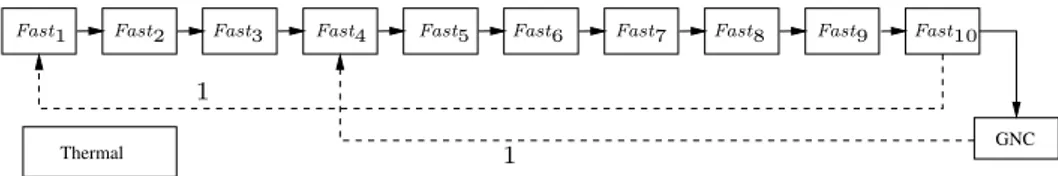
The specification of the space flight application was provided under the form of a set of AADL [18] diagrams, plus textual information defining specific inter-task communication patterns,
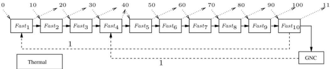
Thermal GNC Fast2 Fast3 Fast4 Fast5 Fast6 Fast7 Fast8 Fast9
1 1
Fast1 Fast10
Figure 5 The Simple example.
determinism requirements, and a description of the target hardware architecture. In this section we use the simpler version of the specification (with fewer tasks), the results on the full example being provided in Section 7.
Our first step was to derive a task model in our formalism. This modeling phase showed that the initial system was over-specified, in the sense that real-time constraints were imposed in order to ensure causal ordering of tasks instances using AADL constructs. Removing these constraints and replacing them with (less constraining) data dependencies gave us more freedom for scheduling, allowing for a reduction in the number of partition changes. The resulting specification is presented in Figure 5.
Our model, named Simple represents a system with 3 tasks Fast, GNC, and Thermal. The periods of the 3 tasks are 10ms, 100ms, and 100ms, respectively, meaning that Fast is executed 10 times for each execution of GNC and Thermal. The hyperperiod expansion described in Section 4.1.2 replicates task Fast 10 times, the resulting tasks being Fasti, 1 ≤ i ≤ 10. Tasks GNC
and Thermal are left unchanged because their period equals the hyperperiod. The direct arcs connecting the tasks Fasti and GNC represent regular (intra-cycle) data dependencies of ASimple.
Delayed data dependencies of depth 1 represent the transmission of information from one MTF to the next. In this simple model, task Thermal has no dependencies.
4.1.3.1 From Non-determinism to Determinism
The design of complex embedded systems usually starts with sets of requirements allowing multiple implementations. Space launchers are no exception to this rule. For instance, the requirements for example Simple do not impose the presence of a delayed arc connecting GNC to Fast4. Instead,
they require that there exists an i such that the feedback from GNC to Fasti is performed under
a given latency constraint.
But determinism has its advantages: As explained in Section 3.1.2, it largely simplifies debugging and testing. Moreover, the determinism of the functional specification allows for a significant decoupling of software development, including verification and validation steps, from allocation and scheduling choices.
This is why a deterministic functional specification is built early in the development process of space launchers. The first step in this direction is made when Giotto-like rules [25] are used to build a fixed set of data dependencies, thus creating a deterministic functional specification. These rules only depend on the number of tasks before hyperperiod expansion, their relative periods, and a coarse view on the flow of data from task to task. This information can be easily recovered from the requirements and from early implementation choices.
The Giotto-like rules allow the fast construction of a deterministic specification and are easy to understand and implement. However, they do not take into account latency constraints, nor task durations, and thus the initial functional specification may not allow real-time implementation. In our example, the initial dependency pattern did not allow the respect of the latency constraint on the feedback from GNC to Fast. When this happens, the dependencies are modified manually within the limits fixed by the requirements to allow real-time implementation.
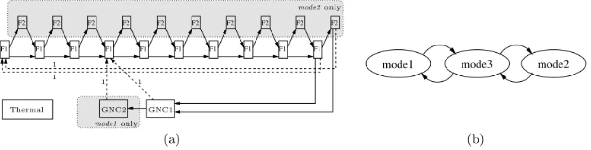
F2 F2 F2 F2 F2 F2 F2 F2 F2 F2 F1 F1 F1 F1 F1 F1 F1 F1 F1 F1 1 1 1 1 GNC1 GNC2 Thermal mode2 only mode1 only mode3 mode2 mode1 (a) (b)
Figure 6 Example 3: Dataflow specification with conditional execution (a) and possible mode
trans-itions (b).
But these manual modifications come at a cost, especially when they must be done late in the design flow, requiring the re-validation of the whole design. This cost can be acceptable when the system is first built, which means once every 20 years or so. But once a deterministic implementation is built, it is strongly desired that subsequent modifications of the system preserve unchanged the functionality of system parts that are not modified (and in particular their determinism). If this is possible during the system modification, then the confidence in the modified system is improved and less effort is needed for the re-validation of the system.
In other words, design choices made during the initial implementation become desired properties for subsequent modifications, where they are considered as part of the functional specification. In our example, we assume that the feedback from GNC to Fast4 is such an implementation choice
made in the initial implementation, and which we include in the functional specification. Our algorithms and tool allow the scheduling of such deterministic specifications. For the cases where the requirements are non-deterministic, our algorithms and tool can be used to speed up an otherwise manual exploration of the possible design choices (but this exploration process is not covered in the current paper).
4.1.3.2 Representing Execution Modes
The dependent task system of Figure 5 does not represent execution modes, implicitly assuming that for each task the scheduling will always use its worst-case execution time.
But a space launcher application does make use of conditional execution and execution modes, and the scheduling can be optimized by taking them into account. The difficulty is to allow scheduling in a way that takes into account modes and is also compatible with the execution mechanisms of the launcher. Recall that the number of tasks in the launcher is fixed – 3. Mode changes do not trigger here the start or stop of tasks, as in our example of Figure 2. Instead, they are encoded with changes of state variables that enable or disable the execution of various code fragments inside the 3 tasks.11
In this approach, the only macroscopic property of a task that changes depending on the mode and can therefore be exploited during scheduling is its duration. Representing mode-dependent durations using our formalism requires a non-trivial transformation, detailed through the example in Figure 6.
We assume that our system has 3 modes (1, 2 and 3), the mode 3 being a transition mode between 1 and 2, as shown in Figure 6(b). We assume that the duration of tasks Fast and GNC
11The state change code is also part of the tasks. It can include arbitrarily complex code, such as the step function of an explicit state machine.
depends on the mode. We denote with WCET(τ, P )m the duration of task τ ∈ {Fast, GNC}
on processor P in mode m ∈ {1, 2, 3}. We assume that WCET(Fast, P )3 = WCET(Fast, P )1< WCET(Fast, P )2 and that WCET(GNC, P )3= WCET(GNC, P )2< WCET(GNC, P )1 for all P .
Then, our modeling is based on the use of 2 tasks for the representation of each of Fast and GNC. The first task represents the minimum task duration (WCET) of the two modes, whereas the second task represents the remainder, which is only needed in modes where the duration is longer.
The resulting model is pictured in Figure 6. Here, Fast has been split into F1 and F2, the second one being executed only in mode 2. GNC has been split into GNC1 and GNC2, the second one being executed only in mode 1. The mode change automaton ensures that (GNC2, F2i, 0) ∈ EXSimpleand (GNC2, F2i, 1) ∈ EXSimple for 1 ≤ i ≤ 10, a property that will be
used by the scheduling algorithms of Section 6. In our example we assumed state change code is executed in the first instance of F1.
The method we intuitively defined here for tasks with 2 durations can be generalized. A task having n durations depending on the mode will need an expansion into n tasks.
4.2
Non-functional Properties
Our task model considers non-functional properties of 4 types: real-time, allocation, partitioning, and preemptability.
4.2.1
Period, Release Dates, and Deadlines
The initial functional specification of a system is usually provided by the control engineers, which must also provide a real-time characterization in terms of periods, release dates, and deadlines. This characterization is directly derived from the analysis of the control system, and does not depend on architecture details such as number of processors, speed, etc. The architecture may impose its own set of real-time characteristics. Our model allows the specification of all these characteristics in a specific form adapted to our functional specification model and time-triggered implementation paradigm.
4.2.1.1 Period
Recall from the previous section that after hyper-period expansion all the tasks of a dependent task system D have same period. We shall call this period the major time frame of the dependent task system D and denote it MTF(D). We will require it to be equal to the MTF of its time-triggered implementation, as defined in Section 3.1.2.
Throughout this paper, we will assume that MTF(D) is an input to our scheduling problem. Other scheduling heuristics, such as those of [39] can be used in the case where the M T F must be computed.
4.2.1.2 Release Dates and Deadlines
For each task τ ∈ TD, we allow the definition of a release date r(τ) and a deadline d(τ). Both are
positive offsets defined with respect to the start date of the current MTF (period). To signify that a task has no release date constraint, we set r(τ) = 0. To signify that it has no deadline we set d(τ) = ∞.
The main intended use of release dates is to represent constraints related to input acquisition. Recall that in a time-triggered system all inputs are sampled. We assume in our work that these sampling dates are known (a characteristic of the execution platform), and that they are an input to our scheduling problem. This is why they can be represented with fixed time offsets. Under
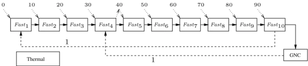
Thermal GNC
Fast2 Fast3 Fast4 Fast5 Fast6 Fast7 Fast8 Fast9
1 1
Fast1 Fast10
0 10 20 30 40 50 60 70 80 90
Figure 7 Real-time characterization of the Simple example (MTF = 100 ms).
these assumptions, a task using some input should have a release date equal to (or greater than) the date at which the corresponding input is sampled. The inputs themselves (their values) are not explicitly represented (they are implicitly used by the task subjected to the associated release dates).
End-to-end latency requirements are specified using a combination of both release dates and deadlines. End-to-end latency constraints are defined on flows, which are chains of dependent task instances. Formally, a flow φ is a sequence of task instances τk1
1 , τ k2 2 , . . . , τ km m such that τ ki i and τki+1
i+1 are connected by a (direct or delayed dependency) for all 1 ≤ i ≤ m − 1. An end-to-end
latency over flow φ requires that the duration between the start of τn+k1
1 and the end of τmn+km is
of less than a given duration l(φ) for all n. In this paper, we require that the end-to-end latency l(φ) is counted from the release date of first task instance τn+k1
1 . This amounts to assuming that
flows start with an input acquisition performed at the release date of the first task.
Under these assumptions, imposing the latency constraint l(φ) on φ is the same as imposing on the last task of φ (τm) the deadline l(φ) + r(τ1) − (km− k1) ∗ MTF.
Before providing an example, it is important to recall that our real-time implementation approach is based on off-line scheduling. The release dates and deadlines defined here are specification objects used by the off-line scheduler alone. These values have no direct influence on implementations, which are exclusively based on the scheduling table produced off-line. In the implementation, task activation dates are always equal to the start dates computed off-line, which can be very different from the specification-level release dates.
4.2.1.3 Modeling of the Case Study
The specification in Figure 7 adds a real-time characterization to the Simple example of Figure 5. Here, MTF(Simple) = 100 ms. Release dates and deadlines are respectively represented with descending and mounting dotted arcs. The release dates specify that task Fast uses an input that is sampled with a period of 10ms, starting at date 0, which imposes a release date of (n − 1) ∗ 10 for Fastn. Note that the release dates on Fastn constrain the start of GNC, because GNC can only
start after Fast10. However, we do not consider these constraints to be a part of the specification
itself. Thus, we set the release dates of tasks GNC and Thermal to 0 and do not represent them graphically.
Only task Fast4 has a deadline that is different from the default ∞. In conjunction with the
0 release date on Fast1, this deadline represents an end-to-end constraint of 140ms on the flow
defined by the chain of dependent task instances
Fast1n→ Fast2n → . . . → Fast10n → GNCn→ Fast4n+1
for n ≥ 0. Under the notation for task instances that was introduced in Section 4.1.1, this constraint requires that no more than 140ms separate the start of the nthinstance of task Fast1
from the end of the (n + 1)thinstance of task Fast
4. Since the release date of task instance Fast1n
Thermal
GNC Fast2 Fast3 Fast4 Fast5 Fast6 Fast7 Fast8 Fast9
1 1
Fast1 Fast10
0 10 20 30 40 50 60 70 80 90 100 110
Figure 8 Adding 3-place circular buffer constraints to our example.
terminates 140ms after the beginning of the MTF of index n. This is the same as 40ms after the beginning of MTF of index n + 1 (because the length of one MTF is 100ms). The deadline of Fast4 is therefore set to 40ms.
4.2.1.4 Architecture-dependent Constraints
The period, release dates and deadlines of Figure 7 represent architecture-independent real-time requirements that must be provided by the control engineer. But architecture details may impose constraints of their own, to be modeled using release dates and deadlines.
We provide here only one such example taken from the case study: Assume that the samples used by task Fast are stored in a 3-place circular buffer. At each given time, Fast uses one place for input, while the hardware uses another to store the next sample. Then, to avoid buffer overrun, the computation of Fastn must be completed before date (n + 1) ∗ 10, as required by the new
deadlines of Figure 8. Note that these deadlines can be both larger than the period of task Fast,
and larger than the MTF (for Fast10). By comparison, the specification of Figure 7 corresponds
to the assumption that input buffers are infinite, so that the architecture imposes no deadline constraint. Also note in Figure 8 that the deadline constraint on Fast3 is redundant, given the
deadline of Fast4and the data dependency between Fast3 and Fast4. Such situations can easily
arise when constraints from multiple sources are put together, and do not affect the correctness of the scheduling approach.
Real-time requirements coming from the control engineers and those due to the architecture are represented using the same constructs: period, release dates, deadlines. By consequence, the scheduling algorithms of the following sections will make no distinction between them.
4.2.2
Worst-case Durations, Allocations, Preemptability
We also need to describe the processing capabilities of the various processors and the bus. More precisely:
For each task τ ∈ TD and each processor P ∈ Procs(Arch) we provide the capacity, or duration
of τ on P . We assume this value is obtained through a worst-case execution time (WCET) analysis, and denote it WCET(τ, P ). This value is set to ∞ when execution of τ on P is not possible.
Similarly, for each data type typea used in the specification, we provide a worst-case commu-nication time estimate WCCT(typea) as an upper bound on the transmission time of a value
of type typea over the bus. We assume this value is always finite.
Note that the WCET information may implicitly define absolute allocation constraints, as WCET(t, P ) = ∞ prevents t from being allocated on P . Such allocation constraints are meant
to represent hardware platform constraints, such as the positioning of sensors and actuators, or designer-imposed placement constraints. Relative allocation constraints can also be defined, under the form of task groups which are subsets of TD. The tasks of a task group must be allocated
on the same processor. Task groups are necessary in the representation of mode-dependent task durations, as presented in Section 4.1.3 (to avoid task migrations). They are also needed in the transformations of Section 5.
Our task model allows the representation of both preemptive and non-preemptive tasks. The preemptability information is represented for each task τ by the flag is_preemptive(τ). To simplify the presentation of our algorithms, we make in this paper two simplifying assumptions: that bus communications are non-interruptible and that preemption and partition context switch costs are negligible.
4.2.3
Partitioning
Recall from Section 3.2 that there are two aspects to partitioning: the partitioning of the application and that of the resources (in our case, CPU time). On the application part, we assume that every task τ belongs to a partition partτ of a fixed partition set Part = {part1, . . . , partk}.
Also recall from Section 3.2 that CPU time partitioning, i.e the time windows on processors and their allocation to partitions can be either provided as part of the specification or computed by our algorithms. Thus, our specification may include window definitions which cover none, part, or all of CPU time of the processors. We do not specify a partitioning of the shared bus, but the algorithms can be easily extended to support a per-processor time partitioning like that of TTA [44].
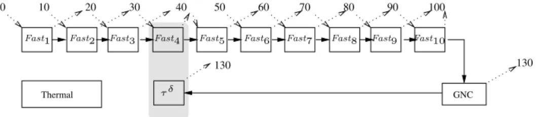
5
Removal of Delayed Dependencies
The first step in our scheduling approach is the transformation of the initial task model specification into one having no delayed dependency. This is done by a modification of the release dates and deadlines for the tasks related by delayed dependencies, possibly accompanied by the creation of new helper tasks that require no resources but impose scheduling constraints. Doing this will allow in the next section the use of simpler scheduling algorithms that work on acyclic task graphs.
The first part of our transformation ensures that delayed dependencies only exist between tasks that will be scheduled on the same processor, so that associated communication costs are 0. Let δ ∈ ∆D and assume that srcδ and dstδ are not forced by absolute or relative allocation
constraints to execute on the same processor. Then, we add a new task τδ to D. The source of
δ is reassigned to be τδ, and a new (non-delayed) dependency is created between srcδ and τδ.
Relation EXD is augmented to place τδ in exclusion with all tasks that are exclusive with srcδ,
and at the same depths. Task τδ is assigned durations of 0 on all processors where dstδ can be
executed, and ∞ elsewhere. Finally, a task group is created containing τδ and dst δ12.
The second part of our transformation performs the actual removal of the delayed dependencies. It does so by imposing for each delayed dependency δ that srcδ terminates its execution before the
release date of dstδ. This is done by changing the deadline of srcδ to r(dstδ) + depthδ∗ MTF(D)
whenever this value is smaller than the old deadline. Clearly, doing this may introduce real-time requirements (deadlines) that were not part of the original specification, which in turn implies that the method is non-optimal (it is a heuristic meant to make the dependent task system acyclic).
Once delayed dependencies are removed, we recompute the deadlines of all tasks. The objective is to ensure that the deadline of a task reflects the urgency of all tasks following it. For instance, task GNC of Figure 8 has no deadline of its own, but it must be finished before the start of Fast4
12The graph is made acyclic by removing the arcs in ∆
D. Nevertheless, code must be generated that corresponds
to these arcs. This generated code creates a variable shared between the helper task and the destination task. These two tasks must therefore be placed on the same processor, which explains the grouping constraint.
130 0 10 20 30 40 50 60 70 80 90 130 100 Thermal GNC Fast10 Fast9 Fast8 Fast7 Fast6 Fast5 Fast4 Fast3 Fast1 Fast2 τ δ
Figure 9 Delay removal result for the example in Figure 8.
in the next cycle. Since the scheduling part of our process will be performed later, we do not know yet when Fast4 will start. Still, we know it cannot start before date 30. Therefore we enforce that
GNC has a deadline smaller or equal to the release date of Fast4 in the next cycle (130).
For dependencies that do not span over multiple cycles, we use a form of deadline re-computa-tion that is similar to the approach of Blazewicz [7], and Chetto et al. [12]. More precisely, the deadline of each task is changed into the minimum of all deadlines of tasks depending transitively on it (including itself), once the delayed dependencies have been removed.
The result of delayed dependency removal and deadline recomputation for the example in Figure 8 is pictured in Figure 9. We have assumed that tasks Fast4 and GNC can be allocated on
different processors, and thus a helper task is needed. The new task group formed of tasks τδ and
Fast4 is represented by the gray box. We assume that all tasks Fastn must be executed on the
same processor, due to an absolute allocation constraint. This is why no helper task is needed when removing the delayed dependency from Fast10 to Fast1.
Note that the two transformations are another source of deadlines larger than the periods. Also note that all the transformations described above are linear in the size of the number of arcs (delayed or not), and thus very fast.
6
Offline Real-time Scheduling
On the transformed task models we apply an offline scheduling algorithm whose output is a system-wide scheduling table defining the allocation of processor and bus time to the various computations and communications. The length of this table is equal to the MTF of the task model.
Our offline scheduling algorithm is a significant extension of the one proposed by Potop et al. [40]. New features are the handling of preemptive tasks, release dates and deadlines, the MTF, and the partitioning constraints. The handling of conditional execution and bus communications remains largely unchanged, which is why we do not present these features in detail. Instead, we insist on the novelty points, like partitioning or the use of a deadline-driven criterion for choosing the order in which tasks are considered for scheduling. The deadline-driven criterion was inspired by existing work by Blazewicz [7] and by Chetto et al. [12]. By comparison with Blazewicz’s works, our algorithm takes into account the MTF, the partitioning constraints, and conditional execution.
6.1
Scheduling Tables
As earlier explained, our algorithm computes a scheduling table. This is done by associating to each task:
A target processor on which it will execute.
A set of time intervals that will be reserved for its execution. A date of first start.