HAL Id: hal-01490731
https://hal.archives-ouvertes.fr/hal-01490731
Submitted on 15 Mar 2017
HAL is a multi-disciplinary open access
archive for the deposit and dissemination of
sci-entific research documents, whether they are
pub-lished or not. The documents may come from
teaching and research institutions in France or
abroad, or from public or private research centers.
L’archive ouverte pluridisciplinaire HAL, est
destinée au dépôt et à la diffusion de documents
scientifiques de niveau recherche, publiés ou non,
émanant des établissements d’enseignement et de
recherche français ou étrangers, des laboratoires
publics ou privés.
Improving Spacecraft Health Monitoring with
Automatic Anomaly Detection Techniques
Sylvain Fuertes, Gilles Picart, Jean-Yves Tourneret, Lotfi Chaari, André
Ferrari, Cédric Richard
To cite this version:
Sylvain Fuertes, Gilles Picart, Jean-Yves Tourneret, Lotfi Chaari, André Ferrari, et al.. Improving
Spacecraft Health Monitoring with Automatic Anomaly Detection Techniques. 14th International
Conference on Space Operations (SpaceOps 2016), May 2016, Daejeon, South Korea. pp. 1.
�hal-01490731�
O
pen
A
rchive
T
OULOUSE
A
rchive
O
uverte (
OATAO
)
OATAO is an open access repository that collects the work of Toulouse researchers and
makes it freely available over the web where possible.
This is an author-deposited version published in :
http://oatao.univ-toulouse.fr/
Eprints ID : 17103
The contribution was presented at SpaceOps 2016 :
http://spaceops2016.org/
To cite this version : Fuertes, Sylvain and Picart, Gilles and Tourneret,
Jean-Yves and Chaari, Lotfi and Ferrari, André and Richard, Cédric Improving
Spacecraft Health Monitoring with Automatic Anomaly Detection Techniques.
(2017) In: 14th International Conference on Space Operations (SpaceOps 2016),
16 May 2016 - 20 May 2016 (Daejeon, Korea, Republic Of).
Any correspondence concerning this service should be sent to the repository
administrator:
staff-oatao@listes-diff.inp-toulouse.fr
Improving Spacecraft Health Monitoring with Automatic
Anomaly Detection Techniques
Sylvain Fuertes1 and Gilles Picart2
Centre National d’Etudes Spatiales (CNES), Toulouse, 31400, France and
Jean-Yves Tourneret3 and Lotfi Chaari4
University of Toulouse (ENSEEIHT-IRIT-TéSA), Toulouse, 31500, France and
André Ferrari5 and Cédric Richard6
University of Nice Sophia-Antipolis, CNRS, Observatoire de la Côte d’Azur, Nice, 06108, France
Health monitoring is performed on CNES spacecraft using two complementary methods: an automatic Out-Of-Limits (OOL) checking executed on a set of critical parameters after each new telemetry reception, and a monthly monitoring of statistical features (daily minimum, mean and maximum) of another set of parameters. In this paper we present the limitations of this monitoring system and we introduce an innovative anomaly detection method based on machine-learning algorithms, developed during a collaborative R&D action between CNES and TESA (TElecommunications for Space and Aeronautics). This method has been prototyped and has shown encouraging results regarding its ability to detect actual anomalies that had slipped through the existing monitoring net. An operational-ready software implementing this method, NOSTRADAMUS, has been developed in order to further evaluate the interest of this new type of surveillance, and to consolidate the settings proposed after the R&D action. The lessons learned from the operational assessment of this system for the routine surveillance of CNES spacecraft are also presented in this paper.
1 Spacecraft Operations Engineer, Operations Sub-directorate, CNES, 18 avenue Edouard Belin, 31401
Toulouse, France, sylvain.fuertes@cnes.fr
2 Spacecraft Operations Engineer, Operations Sub-directorate, CNES, 18 avenue Edouard Belin, 31401
Toulouse, France, gilles.picart@cnes.fr
3 Professor, ENSEEIHT, Telecommunication and Networking, 2 rue Camichel, 31000 Toulouse, France,
jean-yves.tourneret@enseeiht.fr
4 Assistant Professor, University of Toulouse, IRIT-ENSEEIHT, 2 rue Camichel, 31000 Toulouse, France,
lotfi.chaari@enseeiht.fr
5 Professor, Laboratoire Lagrange, Université de Nice Sophia-Antipolis, parc Valrose, 06108 Nice, France,
ferrari@unice.fr
6 Professor, Laboratoire Lagrange, Université de Nice Sophia-Antipolis, parc Valrose, 06108 Nice, France,
I. Introduction
Health monitoring currently performed on CNES spacecraft is based on two complementary surveillance methods applied to house-keeping telemetry (HKTM).
The first one is based on an automatic monitoring of a set of parameters identified as critical during the spacecraft design phase, executed systematically after each reception of new telemetry. This surveillance is mainly based on the Out-Of-Limits (OOL) method which consists of defining a nominal range, with lower and upper thresholds, associated with each HKTM parameter and triggering an alarm if one or more of the parameter acquisitions go out of this nominal range. This method has been enhanced in various ways:
· An anomaly level (“yellow” or “red”) can be added to each monitoring, with respect to the criticality of the anomaly and the response time required for the intervention of the spacecraft operation engineer (SOE) team.
· The surveillance can be conditioned by an event such as the On/Off status of an equipment or its functioning mode.
· A pre-processing can be applied to the data so that the surveillance does not monitor directly the HKTM parameters, but derived parameters computed on ground such as the power spectral density of an analogic parameter or the increments of a counter.
· A filter can be applied so that the alarm is only triggered if several contiguous acquisitions happen to be out of the nominal range.
Relying only on this monitoring method is not sufficient, as it is inherently ineffective to detect an abnormal behavior of a parameter that stays within its surveillance range (see Figure 1). More generally this method requires an a priori knowledge of each abnormal behavior expected, each monitoring being explicitly programmed to detect a particular anomaly signature.
The second monitoring method is based on an aggregation of statistical features (including daily minimum, maximum and mean) of another set of parameters, generated and analyzed monthly. This latter follow-up is achieved not only by the SOE team but also by the spacecraft manufacturers’ maintenance team. It allows long-term evolutions due to ageing or seasonal effects to be visualized, as well as exceptional events if the daily statistical features of a parameter have been impacted. However, in addition to the loss of information induced by the supervision of daily statistical features instead of all the parameter recordings, its monthly frequency does not allow an immediate reaction of the SOE team.
In order to address the shortcomings of the current telemetry monitoring system, several approaches based on machine-learning algorithms have been proposed in the literature. The main idea behind these methods is to use the telemetry stored since the spacecraft beginning of life to create a mathematical model of the nominal behavior of the spacecraft, with the underlying hypothesis that the anomalous events in this reference telemetry are rare. The newly acquired telemetry is then confronted with this model in order to determine if the current spacecraft behavior is nominal (or more precisely “as seen before”) or not. These monitoring methods are completely data-driven and, ideally, do not make any assumption on the parameters behavior during an anomaly or during the nominal functioning of the spacecraft.
In 2013, CNES started an experiment with an ESA tool, named Novelty Detection1, based on a K-Nearest Neighbor outlier detection algorithm. Novelty Detection was able to detect some abnormal events in the telemetry used for its evaluation. However, the method was not directly applicable to symbolic parameters (i.e., parameters that represent a status or a functional mode of a spacecraft equipment instead of a physical quantity).
In 2014, a research and development study was initiated by CNES, in collaboration with the French laboratory TeSA (TElecommunications for Space and Aeronautics), in order to study how other anomaly detection techniques could be applied to telemetry monitoring. The research focused on outlier detection methods, classification methods, and pre-processing techniques able to represent efficiently the behavior of a parameter. During this study, a prototype based on the One-Class Support Vector Machine (OC-SVM) method was developed and showed encouraging results regarding its ability to detect actual anomalies that had slipped through the existing monitoring net. This work has led to the development of a software called NOSTRADAMUS (New Operational SofTwaRe for Automatic Detection of Anomalies based on Machine-learning and Unsupervised feature Selection) that is able to process and monitor hundreds of HKTM parameters in order to test the proposed detection method on a significant amount of telemetry measures.
This paper is organized as follows. Section II presents the detection algorithm developed during the R&D study with TeSA. Section III describes the validation and the adjustment of the proposed method. Section IV is dedicated to the description of NOSTRADAMUS. Finally Section V presents the lessons learned from the operational use of NOSTRADAMUS for the monitoring of spacecraft operated by CNES.
II. A telemetry monitoring method based on a machine-learning algorithm
The R&D study was applied to the analysis of HKTM (House Keeping TeleMetry) parameters recorded permanently by a spacecraft in order to monitor its health. We proposed a method performing anomaly detection on one parameter at a time, as opposed to analyzing the simultaneous behavior of a given set of parameters.
First, a learning phase is required to construct the nominal behavior model of each HKTM parameter. In order to do so, a reference telemetry dataset (learning dataset) must be provided to the algorithm. The processing applied to the parameter acquisitions can be synthetized as follows:
· First, a pre-processing transforms the time-series acquisitions of a parameter into a multidimensional scatter plot, each point being a vector of features.
· Then, the dimension of the scatter plot is reduced by a Principal Component Analysis (PCA).
· Finally, a decision frontier is fitted around the scatter plot by a One-Class Support Vector Machine (OC-SVM) algorithm.
Once the nominal behavior models have been obtained, anomaly detection is performed on new telemetry by applying the same pre-processing and dimension reduction to the data, and determining whether the resulting data lie inside or outside the decision frontier.
A. Pre-processing
1. Data segmentation
First, measurements are segmented in order to build windows with a fixed period of time (100 mn or 24 hours, for instance). Then, some features that will be described in Section II.A.3 are computed for each time window in order to obtain a multidimensional scatter plot, where each point represents a time window. One of the major interests of segmentation and feature computation is to synthetize the information contained in a segment of time, allowing the detection not only of singular points, but also of an atypical set of points even if each point taken individually seems normal.
2. Time window management
The recording frequency of HKTM parameters may vary for expertise purposes: for instance, an investigation on a particular equipment may require a zoom of a telemetry packet at a higher frequency during one hour. This may affect the features calculated on the parameters belonging to this packet over each time window covering the zoom (e.g. increasing the maximum or the minimum observation due a higher recording sampling).
Moreover data may also be jammed because of telemetry “holes” that may happen when some telemetry packets are lost during the download of recorded HKTM over a ground station. Features computed for the time windows containing missing data may have abnormal values.
Since both zooms and telemetry holes are quite rare, it was decided to simply remove the time windows that do not contain the expected number of recorded data.
3. Feature computation
Although feature computation is a standard data pre-processing before using anomaly detection methods, we took advantage of this study to implement and test the application of advanced features to spacecraft telemetry. Frequency features have been added to statistical features and extrema that are used conventionally for anomaly detection. For symbolic parameters, dedicated features have been introduced. The main features used in this study are the following:
· Statistical parameters: mean, standard deviation, skewness, kurtosis · Minimum, maximum
· Energy :
E =
"!#
"$
%(&)
'*! (1)
where N is the number of acquisitions in a time window, and+$(&) denotes the nth acquisition. · Spectral distribution of energy:
F,= - .X/012.%3+++++++4 = 53 … 3 6
7 8
91*7:;8 (2)
where+F,is the energy in the ith frequency sub-band, 01 is the normalized frequency, X/012 is the Fourier transform of the acquisitions obtained with the normalized frequency 013 and 6+is the number of energy sub-bands.
· Average crossing:
P =
"!#
"'*!5
<(')><? (3) where+$@ is the mean of the acquisitions in a time window· Transition probability between states (for symbolic parameters only) · Frequency of occurrence of each state (for symbolic parameters only)
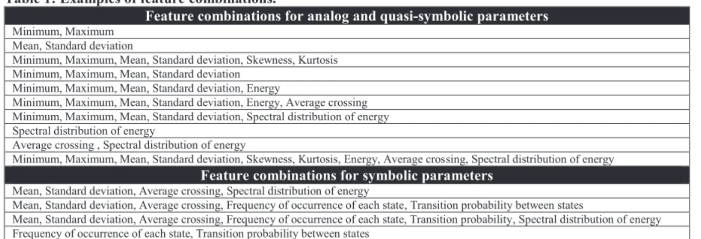
Several combinations of features have been considered for each class of parameters which arouse from this study: analog, symbolic and quasi-symbolic (that are halfway between analog and symbolic parameters: see Section III.A.1 for an example). Table 1 gives examples of feature combinations that were considered for this R&D study.
Table 1: Examples of feature combinations.
Feature combinations for analog and quasi-symbolic parameters
Minimum, Maximum Mean, Standard deviation
Minimum, Maximum, Mean, Standard deviation, Skewness, Kurtosis Minimum, Maximum, Mean, Standard deviation
Minimum, Maximum, Mean, Standard deviation, Energy
Minimum, Maximum, Mean, Standard deviation, Energy, Average crossing Minimum, Maximum, Mean, Standard deviation, Spectral distribution of energy Spectral distribution of energy
Average crossing , Spectral distribution of energy
Minimum, Maximum, Mean, Standard deviation, Skewness, Kurtosis, Energy, Average crossing, Spectral distribution of energy
Feature combinations for symbolic parameters
Mean, Standard deviation, Average crossing, Spectral distribution of energy
Mean, Standard deviation, Average crossing, Frequency of occurrence of each state, Transition probability between states
Mean, Standard deviation, Average crossing, Frequency of occurrence of each state, Transition probability, Spectral distribution of energy Frequency of occurrence of each state, Transition probability between states
4. Data normalization
Since the recorded data provide HKTM parameters with different dynamic ranges, the features themselves do not have naturally homogeneous ranges. For instance, a parameter that has high values will inevitably be awarded a high value for its “maximum” feature.
In order to guarantee good performances of the outlier detection methods, we chose to normalize beforehand the features with respect to their mean and standard deviation. This standard preprocessing guarantees that all the features contribute equally to the decision process independently of the parameter dynamics.
B. Dimensionality reduction
Dimensionality reduction consists of mapping the feature vectors belonging to a p-dimensional space to a lower dimensional subspace of dimension q < p. The interest of this operation is first to reduce the computational cost of the processing but also to face the curse of dimensionality. Indeed, it is well known that increasing the number of features does not necessarily improve the performance of an anomaly detection rule (see Ref. 2 for an interesting discussion related to this problem).
The anomaly detection method proposed in this paper uses one of the most popular linear feature extraction methods, referred to as Principal Component Analysis (PCA). The PCA computes the eigenvectors of the covariance matrix of the original p-dimensional feature vectors. The original feature vectors are then projected onto the eigenvectors associated with the q largest eigenvalues [λ1,…,λq] of the covariance matrix in order to lose the least
information possible. More precisely, the number of eigenvectors q is selected such that 95% of the information contained in the different features is preserved, according to Eq. (4)
#CBDGAB
#HBDGAB
I JKLM
(4)The PCA determines the subspace such that the projected features are the closest (in terms of the mean square error) to the original features.
C. Nominal behavior modelling with OC-SVM
The fundamental anomaly detection problem is based on a one-class classifier, trained with a nominal dataset. An anomaly is detected when the corresponding data is classified as an element that does not belong to the nominal class. Several approaches exist to determine a nominal class from a training dataset. This may be accomplished by estimating the probability density function of the data3, by using neural networks4, or by using one-class support vector machines (OC-SVM)5 which is the algorithm considered in this work.
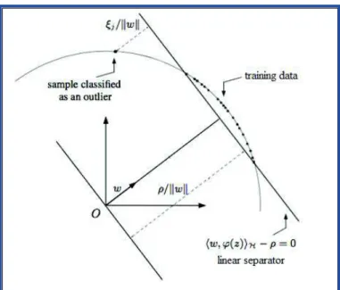
The problem to solve in order to perform anomaly detection is to find a decision frontier around the training dataset, as illustrated in Figure 2. The strategy adopted by OC-SVM, represented in Figure 1, is to map the data in a higher-dimensional feature space H according to a transformation φ, and to find in this space a linear separator (defined by Eq. (5)) that separates the training data, considered as mostly nominal, from the origin with the maximum margin. The frontier separating the normal data points from the anomalies is defined as:
Figure 1. Illustration of the OC-SVM principle. The problem to solve is to find a linear separator in a high-dimensional space that separates the training data from the origin with the maximum margin, while limiting the number of training data classified as abnormal.
We shall now focus on the optimization problem that has to be solved in order to get the parameter vector w and the threshold ρ. On the one hand, the distance that separates the hyperplane from the origin must be maximized. On the other hand, the number of training data classified as abnormal data has to be minimized. Based on these principles, the separator is found by solving the following problem:
min
V3W3Y7+
!%+ ZOZ
%[
\"!# ]
",*! ,T U
(6)subject to the constraints
NO3 Q($,)RS^ U T ],+3+++],^ J (7) where! ν is a relaxation factor that can be interpreted as the fraction of training data allowed to be outside of the nominal class. In engineering terms, ν is the a priori proportion of abnormal data in the training dataset.
Explicitly mapping the input data $, into a high dimensional space _ with Q can make the problem intractable due to high computational cost. Instead of explicitly defining Q and computing+Q($,), an efficient solution known as the “kernel trick” consists of using a kernel function to replace the inner products in the problem to solve. The definition of a kernel function is sufficient to map the data from the original space to the high dimensional space+_. Practically speaking, the choice of the kernel function will define the shape of the frontier around the training data. For this application, we used the Gaussian kernel, one of the most popular kernels for OC-SVM:
`($3 $a) = exp+(TbZ$ T $cZ%)+++ (8)
where!b is a control parameter that adjusts the regularity of the frontier around the training data.
Finally, once the separator has been found, determining whether new data samples are nominal or abnormal is an easy task as it only consists of testing whether it falls inside or outside the frontier. The decision function is then:
0($) = +d4f&(`(O3 $) T +U)+ (9) Some examples of decision frontiers obtained with different values of γ and ν are displayed in Figure 2.
Figure 2. Examples of decision frontiers computed with OC-SVM. Only two features were used so that the data scatter plot and the frontier can be represented in 2D. Red curve: decision frontier, white points: training data, blue points: nominal test data, red points: test data containing anomalies. Figures produced with Scikit-learn6 library for Python.
III. Validation & adjustment of the proposed method
A. Use-cases: two stealth anomalies
In order to validate the proposed method, a dataset containing known anomalies was required. We chose to use the telemetry relative to two actual anomalies that occurred on a spacecraft operated by CNES. In both cases, the monitoring system (OOL and monthly report) failed to detect the abnormal behaviors and the SOE on duty did not have the opportunity to react in a timely manner.
1. Erroneous temperature regulation
The first use-case is relative to an anomaly that occurred on the thermal control system. The SOE team was only alerted of the anomaly after a spacecraft reconfiguration caused by a temperature falling below the on-board FDIR limit. The detailed analysis of the telemetry showed that a dozen of pre-anomaly events were visible up to 16 days before the spacecraft reconfiguration! As it can be seen in Figure 3, during the pre-anomaly events, the monitored temperature is even less likely to trigger a classic OOL detection than during nominal behavior.
The dataset consists of two parameters: the temperature of the thermal line which is a typical analog parameter, and the electrical power injected in the associated heater which is a good example of a quasi-symbolic parameter: even if it is an analog parameter, it can only take values close to either 0W or 3.5W (corresponding respectively to the OFF/ON status of the heater).
Figure 3. Illustration of anomalies in the first dataset. During the nominal functioning, the temperature of the thermal line (green) is regulated between 16°C and 18°C. During the pre-anomaly event, this temperature starts to oscillate at a higher frequency, and never reaches its upper regulation value of 18°C. The pre-anomaly event is also visible on the power injected in the associated heater (blue).
2. Star tracker oscillations
The second use-case deals with a star tracker (STR) which was jammed for several days before it was noticed on ground. No OOL alarm had triggered and the anomaly was simply detected by an SOE during an STR maintenance operation (see Figure 4). It is important to note that this anomaly had not been anticipated at all and that no particular OOL monitoring had been set.
The dataset consists of two symbolic parameters: the validity status of the STR measurements and the current STR operating mode. Three months of data were used for learning and two months (containing two abnormal behaviors) for detection.
Figure 4. Illustration of the anomaly in the second dataset. The anomaly was reflected by a constant restart of the STR (the current operating mode in green keeps moving back to POINTING_TRACK) and oscillations of the measurements validity (in blue) at a high frequency between TRUE and FALSE.
B. Method adjustment
The performance metrics we considered to tune the parameters of the detection algorithm include the number of: · Time windows (N)
· Ground Truth (GT): time windows containing actual anomalies · True Positives (TP): time windows correctly identified as abnormal · False Alarms (FA): time windows incorrectly identified as abnormal
· Non Detections at Window Level (ND-WL): time windows incorrectly identified as nominal
· Non Detections at High Level (ND-HL): non-detection of an abnormal phenomenon spread over several time windows.
Table 2 and Table 3 give some results obtained during one of the anomaly detection campaigns.
Table 2: First example of anomaly detection results. Influence of the time window size on the performance metrics for an analog parameter and for a given set of detection parameters.
Window size N GT TP FA ND-WL ND-HL 4 mn 5630 118 56 222 0 62 10 mn 2252 53 43 0 0 10 50 mn 451 15 11 0 0 4 100 mn 226 8 8 0 0 0 1440 mn 16 3 2 2 2 1
Table 3: Second example of anomaly detection results. A significant impact of the feature selection can be observed on the performance metrics for a quasi-symbolic parameter (QCC_P_RECH_HL05). The spectral distribution of energy seems to be a major feature for the outlier detection of quasi-symbolic parameters.
Features GT TP FA ND-WL ND-HL Minimum, Maximum, Mean, Standard deviation 8 3 44 6 6 Minimum, Maximum, Mean, Standard deviation, Spectral distribution of energy 8 8 51 0 0 Spectral distribution of Energy 8 8 2 0 0 These sets of tests were very informative and helped not only to choose the best features for each type of parameters, but also to tune the parameters of the OC-SVM algorithm such as the size of the time windows. Those results are preliminary and need to be consolidated with larger sets of HKTM data.
C. Comparison with k-NN based detection method
The R&D study ended with a comparison between the OC-SVM and the k-Nearest Neighbors (k-NN) classification methods. The k-NN method we considered is based on the Local Outlier Factor7 (LOF), which is an algorithm used for finding anomalous data points by measuring the local density at a given data point with respect to its neighbors. By comparing the local density at a data point to the local densities at its neighbors, one can identify regions of similar density, and points that have a substantially lower density than their neighbors. These are considered to be outliers. The local density is estimated by the typical distance at which a point can be "reached" from its neighbors. LOF results are quotient-values ranging from 0 to infinity. People usually prefer the Local Outlier Probability8 (LoOP), a method derived from LOF so that the resulting values are outlier probabilities ranging from 0 to 1, which is easier to interpret.
The detection performance proved to be similar for both methods for the analog and quasi-symbolic data sets used for the study. However, for symbolic data we found that the k-NN method provides detection results less reliable than those obtained with the OC-SVM method, with a larger number of non-detected anomalies and false alarms.
Nonetheless, the main advantage of the k-NN method is to offer the possibility to set the threshold of outlier probability very easily in order to reveal the most likely outliers and to “regulate” the number of alarms: an SOE does not need to study all the outliers and can only concentrate on the ones which have the highest outlier probability (larger than 90%, for instance). Conversely, the OC-SVM does not provide a way to identify the most
likely outliers. Thus, all the outliers appear as equal as they are outside the decision frontier, so they will all need to be analyzed by an SOE.
IV. From a prototype to an operational software: NOSTRADAMUS
In order to consolidate the encouraging results obtained during the R&D action, we thought that further testing with a more significant amount of telemetry data was required. However, this could not be easily done with the prototype as any configuration modification (such as the monitored parameters or the choice of the feature sets) required a source code modification.
We decided to develop an operational-ready telemetry surveillance software, NOSTRADAMUS, based on the R&D prototype. The objective of NOSTRADAMUS is dual: consolidate the proposed settings for the detection algorithm with more exhaustive testing on the telemetry of CNES spacecraft, and demonstrate the usefulness of this type of telemetry surveillance for the exploitation phase of a spacecraft. In order to obtain an “operational-ready” demonstrator, the main requirements were:
· The telemetry surveillance must be automatic and compatible with the automation system of CNES CCC
· The user must be able to easily adjust the configuration parameters, and perform the telemetry surveillance with different settings in parallel
· The software must be able to process hundreds of HKTM parameters daily
A. Functionalities
1. Learning and Detection modes
NOSTRADAMUS has two distinct functional modes: learning and detection.
In the detection mode, the detection of atypical behaviors is performed by comparing recently acquired telemetry data to a nominal behavior model learned from the data stored in the telemetry database. The telemetry surveillance should be done promptly after each spacecraft pass, so that the SOE on duty can be alerted quickly if an atypical behavior is detected in the recorded telemetry dumped during the latest pass. In this mode, NOSTRADAMUS processes, in one execution, several hundreds of HKTM parameters acquired during a few hours. When the execution is completed, a result file containing the detections is produced by the program.
The learning mode is used to create the nominal behavior model of each HKTM parameter. Ideally the models should not have to be modified once they have been created. However, our previous experience with the use of Novelty Detection showed that the update of these models with recent telemetry are necessary if we do not want to detect ageing or seasonal effects as atypical behaviors. The creation of new models with the learning mode of NOSTRADAMUS can be done typically on a monthly-basis. This phase requires a large amount of decommuted telemetry (typically 6 months of acquisitions for each parameter) that can raise data storage issues. Consequently, if needed, the creation of a model base can be done sequentially by an automation system: one can extract the telemetry relative to a given parameter from a database, start NOSTRADAMUS in learning mode to create the associated model, erase the telemetry, and continue this process with the next parameter until all models are created.
2. Management of nominal behavior models
The model adjustment parameters such as the nominal period or the set of descriptors to use are defined in a context file. For NOSTRADAMUS, a model is associated to the triplet context-spacecraft-parameter. This means that, for a given spacecraft and a given parameter, several models can be created with different settings and can be used in parallel. It allows us to quickly compare the detection results produced with different settings in order to find which ones lead to the best detection efficiency.
3. Automation
The routine exploitation of CNES spacecraft is highly automatized: an automation tool called AGENDA coordinates the execution of the CCC tools and the transfer of interface files between them. We wanted NOSTRADAMUS to be compatible with this automation system. Consequently, all the information required for its execution are stored into files or given as command-line arguments. It is then possible to define a sequence of operations that will be automatically executed by the AGENDA on a daily basis to perform the telemetry surveillance with NOSTRADAMUS. For instance, during the early hours of each day, the following sequence can be programmed:
· Extract & decommute the telemetry relative to the preceding day
· Perform the telemetry surveillance with NOSTRADAMUS with one or more specified settings · If atypical behaviors are detected, generate an alarm to alert the SOE on duty
Consequently, no additional workload is required to perform the telemetry surveillance, and the SOE team can focus on analyzing the detection results.
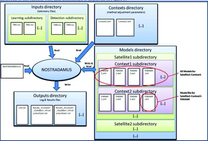
B. Data architecture
All the data required for NOSTRADAMUS execution are stored into files whose content will be briefly described in this section. This data architecture is displayed in Figure 5.
Figure 5. Data architecture of NOSTRADAMUS
1. Input files – decommuted telemetry
The telemetry is given to NOSTRADAMUS as .tsv (tabulation-separated values) files. Apart from the file header, each line represents the acquisition of one or several parameters at a given time. Each group of three columns represents the acquisitions of a given parameter: the first column is the raw value acquired on board, the second one is the physical value (after application of a transfer function to the raw value), while the third one is the significance of the acquisition.
Figure 6. Example of a decommuted telemetry file (.tsv format). Depending on the producing application the information included in the header may vary, except for the first line that lists the parameters included in the file.
These files can be quickly voluminous as the number of parameters requested or the extraction period increases. As an example, a .tsv file containing one week of acquisitions for 50 HKTM parameters acquired at a frequency of 1/32Hz represents roughly 50Mbytes of data. One can easily imagine that it will not be possible to store one year of acquisitions for several hundreds of HKTM parameters in only one file. In order to cope with this limitation, NOSTRADAMUS is able to find, among all the telemetry files at its disposal, the ones that contain the parameters currently being processed and regroup all the acquisitions from these different files.
2. Context files – method adjustment parameters
All the information required to adjust the detection method is defined in context files. Because these files are created or modified by the users, we chose the .xml format as it can be easily compared to a .xsd scheme to detect an involuntary file corruption that could occur during a modification.
The settings that must be defined in the context file include the HKTM parameters to monitor, the window size for segmenting the data, the reference period for the learning phase, and the features that must be computed according to the parameter type (symbolic, quasi-symbolic, analogic).
3. Model files – nominal behavior models
During the learning phase, a model file is created for each parameter to process. It contains particularly the OC-SVM support vectors that define the nominal frontier around the learning data, but also other information required for the detection phase such as the projection vectors computed by the PCA. The settings that were used during the learning phase are also stored in the model so that we can ensure that they have not been changed involuntarily by the user between the learning phase and the detection phase.
4. Result files – detections
Once the detection is over, a result file is produced, containing the detection results and the features computed for each time window and each parameter. The detection results are binary: “OK” if a time window is nominal, “NOK” otherwise.
The tabulated format chosen for this file is a standard format that can be directly imported into PROTON, a data processing tool available in the CNES CCC and sent to PrestoPlot, a fast and efficient time-series plotter.
Figure 7 shows the contents of a result file, and Figure 8 illustrates how it has been processed with PROTON and PrestoPlot in order to superimpose the telemetry and the detection results.
Figure 7. Example of a result file. The file starts with a header which states the parameters that have been analyzed, their type, and the features used. The result lines are organized as follows: window starting date, parameter ID, detection OK/NOK, features values after normalization in the same order as the one stated in the header.
Figure 8. Post-processing of a result file in order to superimpose the telemetry and NOSTRADAMUS detection results. The anomalous event has clearly been identified by NOSTRADAMUS, along with an unwanted false alarm.
V. Lessons learned from the first operational use of NOSTRADAMUS
A. Operational use presentation
The SOE team of one CNES mission has accepted to test this software in parallel with the already existing surveillance means in their CCC. The objective of this experiment is to make sure that most of the outliers correspond either to anomalies or atypical events such as spacecraft maintenance operations in order to evaluate the overall relevance of NOSTRADAMUS’ detection results.
A few dozen of HKTM parameters have been selected for the initial use. They have been chosen by the SOE team in order to represent the heterogeneous nature of the multiple data acquired by a spacecraft (temperature, voltage, relay status, spacecraft attitude, etc.). Those candidates belong indifferently to the families of analog, quasi-symbolic and quasi-symbolic parameters.
Outlier detection is performed with NOSTRADAMUS on a weekly basis. Each time window corresponding to an outlier is displayed on top of the time evolution of the associated HKTM parameter (see Figure 8). This helps the SOE on duty to determine whether the outlier is a true positive or a false alarm. In case of a true positive, the SOE has to find out if the behavior is expected (e.g., as a result of a ground controlled sequence of operations) or not: if necessary, an anomaly sheet is written similarly to any ground monitoring triggering.
B. Lessons learned & perspectives
1. The requirement for an anomaly score
The first observation made by the SOE team while using NOSTRADAMUS is that the detection is too sensitive. Depending on the temporal evolution of the processed parameter, the detection rate can reach one detection per week of telemetry and per parameter for the most “chaotic” ones. After analyzing the detections, they found out that many of them were false alarms. Needless to say that this surveillance could not be directly applied to thousands of HKTM parameters.
The high sensitivity of NOSTRADAMUS can be easily explained by the core principle of the OC-SVM method: the detection frontier only depends on the support vectors that are part of the learning data points. Thus, this frontier cannot be wider than the learning scatter plot. Furthermore, the decision equation (Eq. (9)) only gives a binary result (inside or outside the frontier). Any feature vector that falls outside the decision frontier is considered as atypical, regardless of the distance between the frontier and the vector to be tested.
We are currently modifying the implementation of the OC-SVM method in NOSTRADAMUS in order to compute an anomaly score along with the binary detection results. This anomaly score can be seen as the distance between the vector to be tested and the decision frontier. This modification will provide two advantages for the user:
· It will be possible to easily control the overall detection sensibility
· Among all the detections, the SOE team will be able to focus on the most abnormal ones (i.e., the ones with the highest anomaly score)
2. The “black-box” effect
The simplicity of the “classic” rule-based OOL telemetry surveillance allows the SOE on duty to know immediately why an alarm has triggered by looking at the definition of the given surveillance. When machine-learning algorithms are used, this is no longer the case. A detection means that the evolution of a given parameter during a given time window is more or less different from what has been learned from the reference telemetry. This “black box” effect induces an enormous change in the SOE habits, and can be prejudicial regarding the acceptance of this new surveillance method.
We believe that a post-processing of the detection results is mandatory so that a detection result can be translated into information understandable by the user. Such a post-processing could be for instance a representation of the position of each feature of the test vector compared to the distribution of the learning data features, via a histogram plot.
3. The interest of a semi-supervised learning
The proposed detection method is based on an unsupervised learning phase, which means that the learning data has not been analyzed by the SOE in order to flag each time-period as nominal or anomalous (unlabeled data). This is a strong requirement as it would be impossible for the SOE team to analyze thoroughly all the telemetry produced by a spacecraft.
However, each time window detected as atypical by NOSTRADAMUS will be analyzed by the SOE, as for a classic OOL alarm. The conclusion of this analysis (actual abnormal event or false alarm) should be injected into the
detection method so that the algorithm becomes increasingly reliable. The decision frontier would then depend both on the unlabeled learning dataset and on the user’s feedback: this is called semi-supervised learning.
A simple way to take into account the user’s feedback is to include time windows identified as false alarms in the learning data for the next model update, and to exclude time windows containing abnormal events. However, we found that doing so was not sufficient as some “recurrent-but-not-so-frequent” operations were always detected as atypical by NOSTRADAMUS, even if they had been included in the learning dataset.
A real implementation of semi-supervised learning for NOSTRADAMUS would be to locally modify the decision frontier computed by the OC-SVM algorithm with respect to each user feedback regarding a detection. This represents mathematical challenges that have not been addressed in our work.
4. Multivariate anomaly detection
For simplicity reasons, the proposed method performs anomaly detection parameter per parameter. Thus, the physical correlations that exist between the different HKTM parameters are not taken into account. Our experience shows that most of our actual in-orbit anomalies have an impact on several quantities acquired by the spacecraft. For instance, a friction increase inside a reaction wheel would also cause its temperature to rise. By grouping parameters according to their sub-systems and analyzing them collectively, we believe that we can make the detection more efficient. An anomaly could then be detected as an atypical behavior for several parameters at the same time, or as a significant change in the correlations between parameters.
This multivariate approach could be tested in a basic way with NOSTRADAMUS by considering that a time window is abnormal for a sub-system only if it was detected as atypical for several parameters of the sub-system.
VI. Conclusion
Based on the observation that classical spacecraft health monitoring systems sometimes failed to alert the SOE teams when early signs of equipment failure showed up on its spacecraft, CNES decided to study in collaboration with TESA the interest of machine-learning based surveillance methods. The principle of these methods is to use the HKTM recorded by the spacecraft to construct mathematical models of its nominal functioning. With this type of surveillance, any evolution of parameters that differs from what has been recorded before should theoretically be detected.
CNES has implemented such a monitoring method within a software called NOSTRADAMUS in order to evaluate its pros and cons thanks to an extensive testing on a large scale of telemetry data. The first results showed NOSTRADAMUS effectiveness to detect abnormal behaviors that were not immediately detected by our current monitoring system. However, we have to face a substantial number of false alarms along with the correct detection of anomalies. In addition, the operational assessment of NOSTRADAMUS for the routine surveillance of CNES spacecraft allowed us to identify key functionalities that are required before this type of surveillance can be fully accepted and trusted by the operational teams.
This new kind of surveillance can be a good complement to standard spacecraft monitoring systems, enabling the SOE team to detect early signs of anomalies on a spacecraft. With earlier detection, the operational teams will have more time to take appropriate actions before a definitive failure occurs. This is particularly interesting for critical missions, where a high level of availability is required.
Our short-term work will be dedicated firstly to the adjustment of NOSTRADAMUS settings with the goal of reducing the false alarms rate, and then to the implementation of data post-processing so that an SOE can understand why the evolution of a parameter in a given time window has been detected as abnormal. In addition, we plan to support a PhD thesis in order to propose other anomaly detection methods that can be applied to spacecraft health monitoring, with a focus on multivariate anomaly detection and semi-supervised learning so that the algorithm becomes smarter thanks to user’s feedback about the detection results.
Acknowledgments
The authors would like to thank Jean François Rolland and Didier Semeux from ATOS for their fruitful collaboration to the NOSTRADAMUS development, as well as Loraine Chlosta from CNES for her involvement in this project.
References
1
Martinez-Heras, J. A., Donati, A., Kirsch, M. G. F., and Schmidt, F., “New Telemetry Monitoring Paradigm with Novelty Detection”, Proceedings SpaceOps 2012 Conference, AIAA, Stockholm, 2012.
2
Jain, A. K., Duin, R. P. W., and Mao, J., “Statistical Pattern Recognition: A Review,” IEEE Trans. Pattern Anal. Machine Intell., vol. 22, no. 1, Jan. 2000, pp. 4-37.
3
Parzen, E. “On estimation of a probability density function and mode”, Annals of Mathematical Statistics, vol. 33, no. 3, 1962, pp. 1065-1076.
4
Moya, M., Koch, M., and Hostetler. L., “One-class classifier networks for target recognition applications”, Proceedings World Congress on Neural Networks, 1993, pp. 797-801.
5
Schölkopf, B., Platt, J. C., Shawe-Taylor, J., Smola, A. J., and Williamson, R. C., “Estimating the support of a high-dimensional distribution”, Neural Computation, vol. 13, no. 7, 2001, pp. 1443-1471.
6 Pedregosa et al., Scikit-learn: Machine Learning in Python, JMLR 12, pp. 2825-2830, 2011.
7
Breunig, M. M.; Kriegel, H.-P.; Ng, R. T.; Sander, J. (2000). LOF: Identifying Density-based Local Outliers (PDF). Proceedings of the 2000 ACM SIGMOD International Conference on Management of Data. SIGMOD. pp. 93–104.
8
Kriegel, H.-P.; Kröger, P.; Schubert, E.; Zimek, A. (2009). LoOP: Local Outlier Probabilities (PDF). Proceedings of the 18th ACM conference on Information and knowledge management. CIKM '09. pp. 1649–1652