HAL Id: hal-02083447
https://hal.archives-ouvertes.fr/hal-02083447
Submitted on 28 Apr 2021
HAL is a multi-disciplinary open access archive for the deposit and dissemination of sci-entific research documents, whether they are pub-lished or not. The documents may come from teaching and research institutions in France or abroad, or from public or private research centers.
L’archive ouverte pluridisciplinaire HAL, est destinée au dépôt et à la diffusion de documents scientifiques de niveau recherche, publiés ou non, émanant des établissements d’enseignement et de recherche français ou étrangers, des laboratoires publics ou privés.
Gentle Introduction to the Statistical Foundations of
False Discovery Rate in Quantitative Proteomics
Thomas Burger
To cite this version:
Thomas Burger. Gentle Introduction to the Statistical Foundations of False Discovery Rate in Quanti-tative Proteomics. Journal of Proteome Research, American Chemical Society, 2017, 17 (1), pp.12-22. �10.1021/acs.jproteome.7b00170�. �hal-02083447�
1
Gentle introduction to the statistical
foundations of false discovery rate in
quantitative proteomics
Thomas Burger*BIG-BGE (Université Grenoble-Alpes, CNRS, CEA, INSERM), Grenoble, France.
*thomas.burger@cea.fr
Abstract: The vocabulary of theoretical statistics can be difficult to embrace from the viewpoint of computational proteomics research, even though the notions it conveys are essential to publication guidelines. For example, “adjusted p-values”, “q-values” and “false discovery rates” are essentially similar concepts, whereas “false discovery rate” and “false discovery proportion” must not be confused – even though “rate” and “proportion” are related in everyday language. In the interdisciplinary context of proteomics, such subtleties may cause misunderstandings. This article aims to provide an easy-to-understand explanation of these four notions (and a few other related ones). Their statistical foundations are dealt with from a perspective that largely relies on intuition, addressing mainly protein quantification, but also to some extents, peptide identification. In addition, a clear distinction is made between concepts that define an individual property (i.e., related to a peptide or a protein) and those that define a set property (i.e., related to a list of peptides or proteins).
Keywords: discovery proteomics, statistical analysis, FDR, quality control. Manuscript Type: Tutorial
---
1. Introduction
For a number of years, the proteomics community has been concerned with quality control (QC)a
methods that allow it to provide the most reliable biological conclusions possible on the results it produces. In discovery proteomics, where large-scale approaches are now standard, the vast mass of data that is produced daily is difficult to reconcile with an expert-driven, refined, manual analysis. In this context, the role of QC has spread along the entire chain of interdisciplinary expertise, making statistics necessary in places where it was originally not expected. Recently, three publications related to false discovery rate (FDR) illustrated that a better understanding of statistical QC would be beneficial to the proteomics community:
Serang et al.1 explained that the vigorous debates around QC and data analysis when producing
the first drafts of the human proteomes2,3 probably originated from confusions between at least
two FDR-related notions.
We argued4 that one of the methods most commonly used to compute FDRs in Perseus5 may rely
on a distortion of p-values which has already been described in the microarray literature6; we also
explain why these possibly incorrect p-values may nevertheless be compatible with biologically relevant results, in contradiction with what is generally expected of QC tools.
2
The Human Proteome Project consortium7 proposed stringent guidelines to ensure that, in all
publications linked to the project, thorough descriptions of how FDRs were calculated are presented alongside protein lists. Moreover, some additional validation criteria are required for any claim made about a specific protein.
These publications advocate for a better understanding, and more discussions of FDR and related statistical notions. However, statistical vocabulary can be obscure and may cause confusion, which severely hinders these discussions. In fact, statistics is so deeply rooted in mathematics that it remains disconnected from most of its fields of application, ranging from proteomics to social sciences, where similar discussions are regularly published8,9.
Table 1: List of abbreviations used in this article
Acronyms Meaning
QC Quality control
FDP False Discovery Proportion
FDR False Discovery Rate
PSM Peptide-Spectrum Match
PEP Posterior Error Probability
This tutorial is intended for use by computational engineers who work somewhere in the middle of the chain of expertise required for proteomics research, and who represent an increasing proportion of this chain. The aim is to provide them with an easy-to-understand overview of the following notions: p-value, q-value, adjusted p-value, FDR, local-FDR and false discovery proportion (FDP). Proteomics counterparts to some of these notions were introduced a long time ago, when it first became necessary to estimate the number of peptide spectra that were incorrectly identified. However, their connections to the theoretical foundations of statistics were (and remain) not trivial. More recently, these statistical notions also explicitly showed up in the quantification setting, when attempting to determine which proteins are significantly differentially abundant between at least two biological conditions. As the objective of this article is to relate these notions to the proteomics context, while also helping computational proteomics experts to connect with mainstream data analysis methods, the structure of the article has been reversed with regards to history: first, the quantification setting where the statistical notions are straightforwardly involved is presented. Afterwards, we go back to the well-described peptide identification setting to unravel its statistical foundations.
2. The p-value: an answer to a question that was never asked
Let us consider a relative quantification proteomics experiment where the abundances of thousands of proteins are compared between several replicates split between two biological conditions (e.g. mutant vs. wild-type). We will call (see Fig. 1):
Putative discovery: any protein quantified in the experiment;
True discovery: a protein that is differentially abundant between the biological conditions (generally, these proteins are sought for their potential biological interest);
False discovery: a protein that is not differentially abundant between the biological conditions (generally, these proteins lack biological interest in the context of this experiment);
Selected discovery: a protein that has passed some user-defined statistical threshold (generally this protein is expected to be biologically relevant, however, no one knows whether it is or not). Alternatively, true/false negative/positive taxonomy can be used. However, as already discussed10-12,
false positive rate and false discovery rate are different concepts that should not be confused. As the
3
Figure 1: Venn diagram illustrating the different notions presented in Section 2 (best viewed in color).
Logically, any experimental practitioner would expect a statistical procedure to inform on whether each putative discovery can be classed as true or false. In this idealized case, the set of true discoveries and selected discoveries would concur. Unfortunately, as no procedure exists to produce such a binary classification in a completely reliable way, practitioners of many disciplines learned long ago to accept a probabilistic result, and to select a set of discoveries based on a manually-defined threshold on the range of probability values. When using this approach, the question “what is the probability that a putative discovery is false?” naturally arises. In answer to this question, statistical procedures would be expected to provide a small probability value to indicate a true discovery, and a high one to indicate a false discovery. In practice, statisticians compute the significance of a given protein’s differential abundance using a statistical test, which returns a so-called p-value that behaves exactly as mentioned: small for differentially abundant proteins, large for the others. Because of this concordance, the p-value of one’s favorite statistical test could be understood to correspond to the probability that a quantified protein is not differentially abundant. Unfortunately, this is not the case13.
To understand why, we will use a simpler interpretation of probabilities. Although the p-value is an “individual property” - related to a given protein - it is more intuitive to understand a probability value (in general, not necessarily a p-value) as a “set property”, and more precisely, as a proportion. In general terms, the probability that a random experiment will succeed can be expressed as the proportion of success among trials. This intuitive interpretation can be extended to our case. Concretely, “the probability that a putative discovery is false” can be viewed as the proportion of false discoveries among the set of similar putative discoveries:
#{False Discoveries}
#{Putative Discoveries}: = 𝜋0, (1) and which will be referred to as 𝜋0 from now on. This proportion should be low if the putative discoveries considered are true discoveries, and high otherwise. Now, let us compare this proportion to the one reflected by p-values, which reads:
#{{False Discoveries} ∩ {Selected Discoveries}}
#{False Discoveries} (2) Obviously, Eq. (1) and Eq. (2) differ, and it becomes clear that p-values are not meant to quantify the “probability that a putative discovery is false”. In fact, a p-value is an answer to another question entirely: “What is the probability that a given false discovery is included in the set of selected discoveries?”.
4
In practical terms, this question is more complicated to understand and its answer is less interesting. However, this is the answer provided by statistical tests, since it is much simpler to compute. This can be explained as follows: most of the time, the amount of data available is insufficient to precisely estimate 𝜋0, for any possible type of putative discovery. As we will see later, it is often possible to provide rough estimates of this ratio, at least when one considers all the putative discoveries together. However, this 𝜋0 “averaged on the entire dataset” is not accurate enough to allow selection, or not, of each individual putative discovery. This is why, instead of providing a relatively unreliable answer based on a rough estimate, statisticians propose to use a procedure (namely, the statistical test) that provides an answer (the p-value) to a different question. The question answered is more difficult to relate to the original problem, but its answer is more robust.
3. Statistical tests: why having “enough data” is necessary
Statistical tests are based on the idea that false discoveries are extremely frequent, unlike true discoveries, which are scarce. In other words, a true discovery amounts to a notable fact, while a false discovery is a standard observation. Thus, if “enough data” are available (i.e., a large enough number of proteins to test), statisticians can define a “standard” based on false discoveries (which, in statistical jargon, is termed the null hypothesis), and characterize its statistical behavior (by means of a distribution termed the null distribution). However, it is unlikely that the number of true discoveries will be sufficient to precisely characterize their statistical behavior (by means of another distribution). Thus, the duty of statisticians is to determine whether a putative discovery is true or false, by relying only on the null distribution. To achieve so, the hypothesis testing framework classically proposes to quantify the similarity between the putative discovery and the null distribution, by means of a metric called test statistic. Concretely, for any given quantified protein, the expected “standard behavior” is that of non-differential abundance (or at least, that the difference in abundance can largely be explained by random fluctuations). According to the theory, the similarity between a protein (depicted by a vector of abundances grouped in two sets of replicates) and the null distribution should be measured using any statistic from the Student family. As Student’s statistics are difficult to interpret, they are replaced by p-values, with the following interpretation: for a given protein X, a p-value of 1% indicates that only 1% of the false discoveries will be less similar to the “standard behavior of false discovery” than protein X; which can be directly related to Eq. (2).
The development of the traditional hypothesis testing framework is previous to the advent of big data. As explained in the next section, it is now possible to leverage the big data context to better characterize the mixture of true and false discoveries.
4. The FDP: why having “big data” is important
Let us now assume that more data are available than in Section 3 (even if the corresponding number of proteins is not precisely defined yet). Our intuition tells us that the number of observed true discoveries being mechanically greater, it should become possible to build some meaningful statistics on the true discoveries. Although fully specifying their distribution is most of the time not possible (as one does not know which putative discoveries are true or false), this intuition is nonetheless essentially correct: Notably, we will see that at least, it is possible to provide a rough estimate for 𝜋0 (Eq. (1)). Then, on its basis, it becomes possible to estimate another quantity:
#{{False Discoveries} ∩ {Selected Discoveries}}
#{Selected Discoveries} : = FDP (3) Although this equation still does not answer the original question (for each protein, what is the probability that it is a false discovery?), it nevertheless gives an interesting hint, as it answers a related question: among all the selected proteins, how many are false discoveries? In fact, this approach is
5
simply a shift from a question that relates to an individual protein (the probability that it is a false discovery) to a question that relates to the entire set of proteins (the proportion of false discoveries it contains). This shift from “individual property” to “set property” makes it possible to answer the question, and the resulting quantity is referred to as the false discovery proportion (or FDP). At this point, it should be noted that the FDP is often called the FDR in proteomics. However, as we will see below, this is an oversimplification as an FDR does not exactly coincide with the FDP.
First, we have to grasp why it is possible to estimate this FDP. In fact, even if characterizing the behavior of the putative discoveries themselves is a problem (so far, a manageable one for false discoveries, and an insoluble one true discoveries), statisticians have a very precise idea of how their resulting p-values behave:
The p-values for true discoveries are relatively simply characterized: they are small; instead of being spread across the [0,1] interval, they are concentrated in a small region close to 0, as depicted on the histogram shown in Fig. 2a, illustrating a simulated dataset where all the proteins are truly differentially abundant.
The p-values for false discoveries, in contrast, display counter-intuitive behavior: one would expect them to distribute within the upper-range of the [0,1] interval. If this were the case, it should be possible to find a threshold discriminating between low values (true discoveries) and high p-values (false discoveries). However, this frequent idea fails to consider how p-p-values are constructed: a p-value of X% indicates that among false discoveries (and only them), exactly X% of the other p-values will be lower than X%, while the others will be greater. As a result, the p-value for false discoveries must uniformly distribute across the [0,1] interval. Fig. 2b illustrates a simulated dataset where none of the proteins are differentially abundant.
Figure 2: (a) Histogram representing p-values for a dataset in which 100% of proteins are differentially abundant; (b) Histogram representing p-values for a dataset in which the proteins are not differentially abundant.
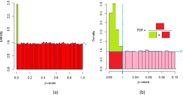
Consequently, if a quantitative dataset contains a proportion 𝜋0 of false discoveries and 1-𝜋0 of true discoveries, the histogram should theoretically look like the one shown in Fig. 3a, which represents a combination of those in Fig. 2. In practice, histograms for real data are not this “clean” (see Fig. 4). However, to understand the logic underlying estimation of the FDP, it is best to work in the “cleaner”
6
theoretical case. If we zoom in on the left-hand side of this histogram (see Fig. 3b), two observations can be made:
First, it would be good to be able to tune the selection threshold to select all the true discoveries, and a minimum number of false discoveries, as illustrated by the vertical dashed line in Fig. 3b; Second, if the dataset is “big enough”, the histogram tends to be smooth. In this case, it becomes
possible to determine a first rough estimate of the FDP by computing the ratio depicted by the colored boxes in Fig. 3b.
To compute this ratio, we must introduce some additional notation. Let: 𝛼 be the user-tuned p-value threshold (the vertical dashed line in Fig. 3b); 𝑚 be the total number of putative discoveries in the dataset;
𝑘 be the number of selected discoveries.
On this basis, a first estimator of the FDP can be simply derived as the proportion, 𝛼, of the total number of false discoveries, 𝑚 × 𝜋0 (i.e., the numerator on the colored-box formula from Fig. 3b), divided by the total number of selected discoveries, 𝑘 (i.e., the denominator):
FDP ≈ 𝛼 × 𝑚 × 𝜋0
𝑘 ∶= FDP̂ (4) Of course, this estimate is rather crude. This is why, one uses the “hat” notation: it is helpful to recall it is not strictly speaking equal to the FDP. However, it illustrates that it is possible to leverage the large amount of putative discoveries to produce a smoother histogram, from which additional information can be extracted.
(a) (b)
Figure 3: (a) p-value histogram for a dataset composed of 100𝜋0% of false discoveries and 100(1-𝜋0)% true discoveries (here,
𝜋0=0.97); (b) zoom on the left-hand side of the histogram, where 𝛼 corresponds to the selection threshold.
As already mentioned, our reasoning was based on a theoretical histogram. In practice, the data seldom distribute exactly as expected. For instance, Fig. 4 shows the p-value histogram for the Exp1_R25_prot dataset14 provided in R package CP4P. This dataset is derived from a differential
analysis of proteins in two groups of three replicates. The protein samples contain an equal background of yeast proteins, into which UPS1 human proteins have been spiked15. In the second condition, the
concentration of UPS1 is 2.5-fold larger than in the first, so that in the end, all the UPS1 human proteins (and only them) should be differentially abundant. After individually testing each protein (either human or yeast), a list of p-values is obtained for which the histogram is shown in Fig. 4.
7
Figure 4: Histogram of the p-values associated with the differential abundances of the proteins from the Exp1-R25-prot dataset14: In red, the yeast proteins from the background, in green, the human UPS1 proteins.
Comparison of the histograms in Fig. 3 and 4 shows that the silhouettes do not matchb. The difference
in behavior between the true and false discoveries is blurred, making it impossible to precisely define 𝛼 and 𝜋0; and thus, to accurately estimate the FDP with Eq. (4). This is why it has been necessary to rely on statistical theory to develop more robust estimators for the FDP, as discussed in the next section.
5. What are FDRs?
Essentially, an FDR is an estimate of the FDP that is endowed with some important statistical properties (see Efron’s book16 for a survey of the subject). Mainly, an FDR must be:
Conservative: i.e., it should not under-estimate the real FDP, or at least, it may do so, but only with a controlled probability. This is essential to ensure that the number of false discoveries selected does not exceed the number estimated (and accepted). In other words, conservativeness is essential to the QC of the biological conclusions.
Asymptotically convergent: i.e., in the long run, the average of a large number of FDR computed on datasets with the same statistical distributions should tend toward an upper-bound of the real FDP.
Statisticians have worked extensively on these properties, but have unfortunately failed to reach a consensus on their precise implementation. For instance, even their mathematical definitions differ slightly depending on whether we use Benjamini and Hochberg’s framework18-21 (BH), or that
developed by Storey and Tibshirani22-26 (ST). However, from the practical viewpoint of proteomics data
analysis, these technical details have little or no influence; in fact, the BH and ST families are similar on many points, and these common elements are those on which it is important to focus.
First, both families are more or less related to the naive estimator of the FDP discussed above (see Eq. (4)). Consequently, FDRs from both families need to estimate 𝜋0.
Second, both families have the same type of “relatively weak” sensitivity with respect to the volatility of the estimate of 𝜋0. Conveniently, it is not essential to precisely determine 𝜋0 (although it would be
b As an aside, we mention that this difference between the theoretical and real histograms is well-known and is
classically referred to as a p-value calibration issue17. It generally has multiple origins, among which: (1) small
number of replicates (here 3 vs. 3) which makes the test hardly robust; (2) dependences between the proteins tested, since protein abundances are not completely independent from one another; (3) sub-optimal preprocessing (for instance peptide misidentifications) which introduce errors that are propagated in the data analysis pipeline. The CP4P package14 provides tools to visualize and limit the effects of incorrect calibration.
p-values F re q u e n cy 0.0 0.2 0.4 0.6 0.8 1.0 0 20 40 60 80 100 120
8
a bonus); what really matters is to avoid its underestimation. This is why, in the original work of Benjamini and Hochberg, they used 𝜋0= 1. This is also why, in the introduction, we spoke about using a rough estimate for 𝜋0. A precise estimation would be necessary to reliably define the probability that a putative discovery is false, but a hand-waving over-estimator is sufficient to produce a good FDR (regardless of whether it is a BH or an ST one). And finally, this explains why numerous statistical works14 have been devoted to defining different 𝜋0 estimates, that can be inserted into the different
BH and ST frameworks.
Third, both families can be cast into the same algorithmic procedure, summarized as follows: 1. Sort putative discoveries by increasing p-values:
𝑝𝑚𝑖𝑛 = 𝑝(1)≤ 𝑝(2)≤ ⋯ ≤ 𝑝(𝑚−1)≤ 𝑝(𝑚)= 𝑝𝑚𝑎𝑥 (5) 2. Walk through the list of p-values from 𝑝(1) to 𝑝(𝑚), and for each 𝑝(𝑘), 𝑘 ∈ [1, 𝑚]:
2.1. Assume that in Eq. (4), one tunes 𝛼 = 𝑝(𝑘) (i.e. 𝛼 is tuned to select exactly the first k discoveries) and compute the resulting naive estimate:
FDP̂ (𝑘) = 𝑝(𝑘)× 𝑚 × 𝜋0
𝑘 (6) 2.2. Store FDP̂ (𝑘) in the 𝑘th cell of an intermediate table
3. Walk through this intermediate table, from 1 to 𝑚:
3.1. Compute the FDR associated to the set of the 𝑘 best discoveries, i.e. the set {protein(1), … , protein(𝑘)}, by applying the following computation:
FDR ({protein(1), … , protein(𝑘)}) = min𝑖≥𝑘(FDP̂ (𝑖)) (7) 3.2. Store the corresponding FDR in the 𝑘th cell of the result table.
4. Walk through the result table from 1 to 𝑚 and stop just before meeting an FDR value that is greater than acceptable (say 𝛽%). Let 𝑁 be the index of this value. The set {protein(1), … , protein(𝑁)} therefore has an FDR of 𝛽%, which means one can roughly assume its FDP is slightly smaller than 𝛽%.
As indicated at the very beginning of this tutorial, q-values, adjusted p-values and FDR are rather similar conceptsc. We will now explain why. If one incorporates Eq. (6) into Eq. (7), one obtains:
FDR ({protein(1), … , protein(𝑘)}) = min𝑖≥𝑘 (
𝑚 × 𝜋0
𝑖 × 𝑝(𝑖)), (8) which underlines FDRs at various decision thresholds can be derived from applying a transform to the list of p-values, leading to the terms adjusted p-value (BH literature) or q-value (ST one).
cTo better understand the theoretical foundations of the concepts presented in this tutorial, and to access the
precise definitions of the various types of FDRs within the BH and ST families, any advanced reader will sooner or later study the corresponding literature, starting with the seminal 1995 paper of Benjamini and Hochberg18,
or even older articles, such as those referenced by Goeman and Solari27. At this point, the reader will find that
the definitions used in this tutorial do not exactly match those in the earliest literature. The reasons for these apparent discrepancies are mainly historical: in fact, q-values and adjusted p-values, as interpretations of the FDR, appeared several years later. Thus, to define the adjusted p-/q-values on top of FDR, one needs a trick: Basically, one first define an intermediate notion, namely, the FDR-level of each putative discovery (an individual property). Then, one defines adjusted p- /q-values/FDRs as a minimum over the FDR-levels beyond the threshold. Let us note that confusions between FDR-levels and FDR often leads to the wrong idea that an adjusted p- /q-value is not an FDR, as its looks like a minimum over several FDR /q-values. However, it is not: taking the minimum FDR-level is equivalent to taking the minimum in Eq. (7), so that, in the end, the original and new definitions concur. To conclude this remark, let us sketch a brief intuition why taking the minimum is required: As explained in Section 4, 𝜋0 is often tune to overestimate the overall proportion of false discoveries in the entire dataset.
9
The problem with this type of naming convention is that it sometimes leads non-statisticians to severely misunderstand the significance of terms. The most common misunderstanding here is that q-/adjusted p-values are merely corrections of p-values, closely connected to them rather than to the concept of FDR. It is of the utmost importance to remember that a p-value is an individual property, while an FDR, an adjusted p-value or a q-value are set properties. Thus, a p-value relates only to the individual putative discovery with which it is associated, and nothing else; if the rows in a table of proteins associated with values are shuffled, or filtered out, or merged with another table, the p-values remain meaningful. In contrast, any FDR, adjusted p-value or q-value relates to a set. Even if it looks like this value is associated with the 𝑘th putative discovery, it is in fact linked to the entire set of
putative discoveries with smaller values. Thus, if the table of proteins is ordered by increasing p-values, the FDR, adjusted p-value or q-value is meaningful (it relates to the set of lines above); but if the lines of the table are shuffled, there is no visually obvious way to relate the FDR, adjusted p-value or q-value to the set to which it corresponds. Similarly, any modification of the data table (for instance, protein filtering on the basis of biological evidence, or merging with another dataset) will make the FDR spurious.
6. Local-FDR: why having “even bigger” data is an advantage
Our line of reasoning so far was as follows: if sufficient knowledge on the behavior of the data has been garnered, “standard behavior” can be defined (known to statisticians as the null hypothesis distribution), and thus each putative discovery can be tested individually. If a large number of putative discoveries are considered simultaneously - as in any high-throughput omics experiment - the p-value distribution (or histogram) can be used to define a conservative estimate of the FDP, termed FDR. This FDR can be used as a QC measure, as an FDR of X% can be used to claim something like: “the proportion of falsely differentially abundant proteins in my protein list is likely to be lower than or equal to X%”. Although useful, this FDR remains a set property that qualifies the entire protein list, whereas an individual QC metric for each protein would be of greater interest. As indicated in the introduction, it is generally not possible to refine the QC metrics for individual proteins; however, with large data volumes, an “in-between” measure can be defined that only fits a restricted subset of putative discoveries, which are to some extent similar.
To understand how, we must assume that, for a given experiment, our protein list appears to be ten times longer than usual. Thus, the list can be clustered into ten homogeneous groups sharing common features. Within each group, the number of proteins remains large enough to allow calculation of a specific FDR for each group, individually, following the line of Section 5.
To define these homogenous groups, a first solution is to rely on any available covariates. For instance, proteins can be grouped according to the number of peptides identifying them (the underlying rationale being that the more peptides identified, the more reliable the quantification). Alternatively, one can rely on the ratio of missing quantitative values, or any other covariate related to the quality of each protein quantification. The FDR computed for a group of “higher quality” would be expected to be smaller than that for a group of “lower quality”.
Another solution is to define the groups according to the test statistics itself. In this case, the proteins are sorted by increasing p-value, and for each possible value, only the subset of proteins belonging to a specific interval around is considered. Thus, a “sliding subset” of proteins emerges rather than a hard clustering into groups. This approach produces a locally defined FDR for each point of the range of p-values, as illustrated in Fig. 5, and is known as local-FDR16. Finally, a local-FDR is a QC measure that
relates to such a small set that it is nearly an individual property. Although it sounds convenient, local-FDR is a double-edged sword. In the limit case where the histogram depicted in Fig. 5 is perfectly smooth (which would require an infinite number of proteins), the local-FDR converges toward the probability that a selected discovery is false. This probability, which we have been looking for since the introduction, finally becomes accessible, at least in theory. However, in practice, infinite data cannot
10
exist; at best, one “only” has a huge volume of data, producing a “reasonably” smooth histogram which is compatible with computation of a fairly robust local-FDR. If the volume of data is not large enough, the histogram profile will be too irregular and local estimates will be unstable. Thus, a trade-off must be sought, between the “locality” of the estimate (the more local the better) and its robustness (the more local, the less robust). Although proteomics researchers classically desire the most refined local QC metrics, it is the computational engineer’s duty to advise the use of more global ones if they are the only ones to be trusted.
Figure 5: Local-FDR is used to estimate the FDP locally, in contrast with the classical FDR (see Fig. 4b), which is a global estimate.
When comparing these two approaches, let us not that local-FDR uses a single null distribution for all the sliding windows, while on the contrary, in the per-group computation of FDR, one commonly uses a specific null distribution for each.
7. Unveiling the statistical foundations of FDR at the identification step
So far, we have only relied on quantitative analysis because it naturally matches the statistical framework of hypothesis testing. However, from a historical perspective, as well as from the viewpoint of data processing, FDR is primarily associated with identification QC. In this setting, the practical goal is to filter out incorrect PSM (peptide-spectrum matches), so as to retain only correct ones. Unfortunately, it is less intuitive to relate the identification QC problem to the hypothesis-testing framework. This state of affairs may lead to misinterpretation of results and, consequently, to spurious conclusions, as recently discussed2.
11
The purpose of this section is not to describe the identification workflow from a theoretical statistics viewpoint. Its objective is more humble. It is only to link the theoretical foundations of FDR to the practical setting of PSM validation. To do so, one needs to find in the PSM validation process different elements that can be considered as counterparts to the building blocks of FDR theory that have been described in Sections 4 and 5. Concretely, one needs to check that (1) true and false discoveries are properly defined; (2) a null distribution is available; (3) a test statistics can be used to derive p-values on which a mixture model equivalent to that of Fig. 3 can be constructed; (4) an estimate of the FDP such as Eq. (4) is available.
(1) True and false discoveries definition. As true discoveries are what we are interested in, they should be defined as correct PSMs. Consequently, false discoveries should be the incorrect PSMs; and putative discovery can therefore be defined as any possible pair of the type {Peptide; Spectrum}, regardless of whether it is correct or incorrect. Thus, the set of putative discoveries is more abstract than in the quantitative analysis, becoming a combinatorial set (i.e., made of a series of possible combinations). (2) Null distribution. If a {Peptide; Spectrum} pair is randomly selected from among all possible pairs, it is highly unlikely to have a correct PSM by chance. In other words, the “standard” is for PSM to be incorrect. However, it is harder to qualify a mismatch than a match; or to paraphrase Leo Tolstoy, “All
correct PSMs are alike; each incorrect PSM mismatches in its own way”. Clearly, this makes it more
difficult to define a “standard” than in the quantification setting (where equal abundance distribution was sought). Fortunately, this difficult task is conducted by most database search engines, so that practitioners need not worry about it.
(3) Test statistics and p-value existence. Unraveling these notions is clearly the most difficult issue: In numerous cases, the test statistics and the p-values are computed within the identification engine, yet, they are not provided. Rather, they are transformed into scores that form the only output accessible to the user. Then, the output score, noted 𝑆𝑖 for the 𝑖th peptide-spectrum pair, is related to a p-value, 𝑝𝑖, by a formula such as the following:
𝑆𝑖 = − 10 log10𝑝𝑖 (9) As a result of this one-to-one correspondence between scores and p-values, to compute an FDR, it is possible to directly work with the histogram of output scores instead of that of p-values, as illustrated in Fig. 6. Concretely, what really matters is to have a mixture model to rely on, and whether it depicts p-values or output scores seldom matters. In fact, the conceptual links between the mixture model and the computation of the FDR are so strong that it is sometimes possible to bypass the p-value computations, and to empirically define the null distribution directly on scores16 (chap. 6). This explains
why, there also exist identification tools where p-value computation is even not performed as an intermediate step. Similarly, to discriminate between correct and incorrect PSMs, numerous post-processing tools (e.g. PeptideProphet28) directly rely on a mixture model of scores as the one illustrated
on the lower right-hand panel of Fig. 6. However, it is very important to keep in mind that there always exists a histogram of p-values that could be used in place of the mixture model, and that this is the very reason why FDR computation is theoretically supported. If this histogram did not exist, there would be no guarantee that conclusions drawn from the mixture model would be valid. For instance, database search engines exist with a scoring system that cannot be directly interpreted in terms of p-values (mainly because PSMs are not scored independently from one another). Some authors29 point
12
Figure 6: Schematic illustration of the conceptual link between identification scores and p-values: The arrows indicate how it is possible to shift between a p-value histogram and a mixture model representation, so that direct FDR computation on the
basis of identification scores is theoretically supported.
(4) FDP estimate. At first glance, this is where the main difference between identification and quantification lies, as the so-called target-decoy approach30 is used instead Eq. (4) to estimate the size
of the red rectangle shown in Fig. 3b. However, from a theoretical viewpoint, the underlying rationale is really similar. The purpose of target-decoy methodology is to artificially create a large number of false discoveries that can be easily traced (because the peptide involved in each {Peptide; Spectrum} pair is a random sequence of amino acids that does not exist in the protein sequence database). As a result, once the practitioner has cut the PSM list at a given score threshold, the PSMs with a real peptide (termed “targets”) can be distinguished from the others (termed “decoys”) to compute the proportion of decoy PSMs. In this scenario, the strong assumption is made that mismatches (involving a real peptide) have the same distribution of scores as the decoy PSMs, so that among the PSMs above the threshold, the number of false discoveries can be derived from the number of decoys31. Although
the approach is empirical, it can be demonstrated fits in the classical FDR framework11,31. However, as
a side effect, the same weaknesses as with the classical FDR computation procedure affect target-decoy approaches: An overly biased estimate of 𝜋0 may affect the results31, the size of the decoy database and the uniformity of sampling of the false discoveries are critical11, the volatility of the FDP
estimate may require a control of the confidence interval31, etc.
8. From peptide level local-FDR to protein-level FDR
In Section 7, we uncovered the relationships between classical statistics-based FDP estimation and target-decoy approaches. We concluded with few weaknesses of the target-decoy approaches, which are directly inherited from statistical theory. Now, we present a more optimistic viewpoint, by leveraging this theoretical connection to define local-FDRs for peptide identification.
13
The first approach applies the same line of reasoning as depicted in Fig. 5 (where the local-FDR is derived from the histogram of p-values) to the histogram of scores (e.g. lower right-hand part of Fig. 6) to produce the computation illustrated in Fig. 7. This procedure returns the so-called posterior error
probability (or PEP), which is already a popular alternative to FDR33-35.
Another approach is to cluster PSMs according to some additional covariate(s), and to provide a specific FDR for each cluster. Reiter et al.36 propose to cluster the target and decoy PSMs based on the
identities of the parent proteins to produce a target-decoy-based estimate of the FDP at PSM level for each protein. As the putative discoveries are split between an enormous number or clusters (as many as proteins), it is rather difficult to gather enough data within each cluster to achieve reliable FDP estimates. Because the size of the dataset is essential to its successful application, the article title indicates that the methodology is applicable with “very large proteomics data sets”. However, its main feature is not that it proposes a PSM-level FDR for each protein, but that it transforms the PSM-level FDRs into a protein-level FDR. This is achieved by modeling each protein by the random draw of a series of colored balls from an urn (say the black balls represent the decoy peptides and the white ones the target peptides). The outcomes of this type of random experiment are known to distribute according to hypergeometric law (with different parameters for correct and incorrect proteins), making it possible to define the “standard behavior” of proteins with respect to the distribution of target and decoy peptides. Consequently, a null hypothesis distribution is produced, making it possible to define protein-level p-values (or scores), and thus an FDR.
Much effort has been devoted in recent years to defining a protein-level FDR. However, it is a complex issue. As recently discussed13, the very definition of truly and falsely identified proteins can be
questioned: is a falsely identified protein absent from the sample? Or is it the result of an inference from incorrectly validated PSMs (even though a protein can be correctly identified on the basis of incorrect peptide-level evidence)? While practitioners expect the first case, the solutions currently available tend to be based on the second.
Figure 7: Applying the concept of local-FDR to the histogram of peptide identification scores produces the concept of PEP.
Another difficulty relates to the following simple observation: to compute an FDR at the protein level, putative discoveries must be defined as putative protein identifications, endowed with a score of known distribution for incorrect identifications (to define the null hypothesis). Unfortunately, analysis
14
is conducted at peptide level and it is therefore necessary to aggregate the peptide-level scores into protein scores, while precisely controlling how the aggregation process influences the distribution of scores (for both true and false identifications). In general, this aggregation remains a very difficult statistical subject, for which only few results are available to date. In the specific case where the dataset is very large, the hypergeometric model, as proposed by Reiter et al.36, can be effectively
applied. For smaller datasets, no strategy dominates the state-of-the-art12 (Sec. 7). As no strategy is
perfect, an additional source of errors may be introduced during aggregation. Then, one runs the risk of increasing the difference between the real FDP and the computed FDR when shifting from peptide-level to protein-peptide-level.
Of course, the expectations of wet-lab researchers for protein-level QC are legitimate, as they are easier to interpret and relate to the biological problem. However, in the meantime, computational experts must determine whether or not this increment of biological interpretability is worth authorizing hidden and unwanted distortion of the QC metrics. To the best of the author’s knowledge, no survey has benchmarked the various protein-level FDRs so far from this angle. Therefore computational experts currently have no material with which they could find a trade-off between the gain in interpretability and the possible loss of accuracy this distortion might produce.
9. Practical recommendations and discussion
In this section, the theoretical background reviewed so far is used to derive some guidelines. However, one should recall that statistical science has developed like many other sciences: First are the foundations, consisting of basic, commonly accepted and rarely discussed knowledge that can be presented in tutorials. From these foundations, different protocols have emerged, based on each individual’s experience: these protocols are somewhat subjective, as two different ones may be equally correct. As a result, unlike the rest of the article, the elements given here remain debatable and amendable. This being noted, a few very practical questions will now be addressed.
1. Concretely, what does “enough”, “big” or “even bigger” data mean? For instance, at what point is it safe to consider the volume of data to be large enough to compute local-FDR?
2. Throughout the text, “user-defined thresholds” were referred to with regards to scores, p-values or FDRs… But how should these thresholds be tuned in practice?
3. When processing real-life datasets, researchers not only focus on the scores or the p-values, but also on an important number of covariates, that are known to be relevant. How can these be accounted for in the statistical framework presented so far?
With regards to the first point, it is at least possible to define orders of magnitude. For example, in Section 3, “enough data” referred to the fact that it was possible to garner sufficient observations to define the null distribution. However, in proteomics, either for identification or quantification, the statistical tests that should be used (and the corresponding null distributions) are well-known: the beta-binomial test for spectral count data37, Student family tests for eXtracted Ion Chromatogram
data, the tests embedded by search engines for identifications, etc. As a result, this issue is practically resolved. Next, we know that “big data” are necessary to compute an FDR, so that the question arises: When does an FDR become meaningful? Intuitively, it is best to avoid talking about a percentage of false discoveries if there are less than one-hundred selected discoveries (what would be the meaning of 1% FDR on a list of 35 proteins?). However, even 100 discoveries may be borderline. In fact, to represent the histogram of the data, as illustrated in Fig. 4, it appears that smoothness requires more than 100 observations; so that a few hundred (e.g. from 500 to 1000) make more sense. Finally, “even bigger data” is required to define local-FDRs. We considered two cases: in the first one, the dataset is binned into N groups for which N separate FDRs are computed, so that one naturally needs to have N times more data to achieve reliable estimates. Otherwise, it may be wiser to forget local-FDR and to stick to more global QC measures. In the other cases where a “sliding set of discoveries” was
15
considered, such as with Efron’s local-FDR or with PEP, the issue relates more to the regularity of the distribution (see Fig. 4) than to the volume of data. Therefore, no simple general rule holds33,16 (Ch. 5,7).
Before addressing the two remaining questions (user-defined thresholds and covariates), let us go back to the reason why FDR is necessary in proteomics. From what we have discussed so far, in statistics
FDR Control mainly relies on an estimation procedure: given a list of 𝑚 discoveries, we first attempt
to estimate an upper-bound of the FDP in the k first elements of the list, ∀𝑘 ≤ 𝑚. Second, on the basis of this estimate, the value for k can be chosen so as to fit with a user-expected FDR value. Basically, once the estimate has been calculated, the FDR control simply amounts to adjusting some threshold to cut the list to the right length.
Conversely, from a proteomics viewpoint, FDR Control is mainly based on filtering procedures: the issue is largely to prevent the spread of false discoveries through the application of stringent procedures derived from some proteomics expertise. To do so, the practitioner defines several knowledge-based filters at PSM-, peptide-, or protein-level: for instance12, mass accuracy, peptide
retention times, peptide length, compliance with digestion rules, a priori amino acid sequences, protein length or a minimal number of matching peptides (e.g. the two-peptide rule). Similarly, at the quantification step, proteins with too many missing values can be filtered out38, as can proteins for
which the fold-change is too low5. These are common good practices which are experimentally proven
to reduce the number of false discoveries. In real terms, they amount to sorting the discoveries according to additional covariates that the practitioner can interpret.
False discovery estimation (the statistician’s viewpoint) and false discovery filtering (the practitioner’s viewpoint) are two different approaches which are both important for QC. First, both of them have drawbacks. As previously explained, false discovery estimation is based on asymptotic theory: even if the FDP will be well-controlled in the long run average, the FDR cannot be used as a precise and rigorous equivalent of the FDP in any single given proteomics experiment. On the other hand, false discovery filtering is no better: even if the filters are plainly sensible, they provide no estimation of the FDP. Second, both approaches are interesting: filtering relates to the practitioner’s capacity to keep a critical eye on his/her own proteomics experiment, to publish the most reliable material. Whereas false discovery estimation provides statistical guidelines which mainly guarantee that results from different articles can be cross-compared, and that different experiments from different researchers involve application of a similar trade-off between the risk of publishing false discoveries and the benefit of publishing the longest possible list of true discoveries.
Finally, the two viewpoints are complementary, and it makes sense to start by filtering out false discoveries, by multiplying stringent procedures, and to subsequently estimate their proportion, on the final filtered list. With this in mind, we will now address the issue of how to tune the p-value/score/FDR thresholds. These thresholds are of little interest in the practitioner’s context of false discovery filtering, but are of prime importance to estimate the number of false discoveries. Thus, depending on who will receive the results of the proteomics analysis, these thresholds may be important, or not. For example:
To publish, it is mandatory to apply a classical threshold (say 1% FDR if the journal does not stipulate a specific value) so as to allow cross-comparisons with other published data, as mentioned above.
If the proteomics analyses are part of a preliminary study, where a good trade-off between false selected discoveries (in a classical QC perspective) and unselected true discoveries (so as to maximize proteome coverage) is sought, then it makes sense to rely on the Receiver Operating Characteristic (ROC) curve39 to define the optimal FDR level.
On the contrary, if the results are sent to a partner lab who only has the funds to manually validate, let us say, 15 proteins, regardless of the number of significantly differential ones, then it is not necessary to compute a FDR at a specific level: the ID of the 15 proteins with the lowest p-value
16
should be transmitted to the lab (keeping in mind that transforming p-values into q- or adjusted p-values does not modify their ranking). Then, computing the PEP for these 15 proteins may be an additional QC metric, the advantage of which will mainly depend on whether the collaborators can interpret it.
Finally, definition of these statistical thresholds is very context-dependent, and they should not be given more than appropriate importance.
Let us now turn to the question of covariates. As it should have appeared to the reader, the theoretical foundations of FDR are already complex without trying to account for any discipline-specific covariates. As a result, computational experts working in proteomics may have a hard time defining asymptotically convergent and conservative estimates that natively incorporate these covariates. However, these covariates are useful for false discovery filtering as proteomics expertise relies on them, and there is no reason to omit them. This is why, during the filtering step, all the covariates can be used to define stringent filters, either by hand, or by relying on machine-learning algorithms (e.g. Percolator40). This
approach should produce a more reliable list of discoveries according to the data owner, on which, as a final QC, an FDR can be computed (based only on the p-values or their related scores, regardless of the other covariates).
10. Conclusions
Over the last few years, the throughput of LC-MS/MS experiments has dramatically increased, so that proteomics has now definitively entered the realm of big data. As a result, computational experts are playing an increasingly significant role in proteomics labs, where they make the link between mass spectrometry expertise and biological expertise. In this context, this article revisited the statistical foundations of several concepts (see Table 2 for a summary), so as to provide computational experts with additional skills when implementing data processing routines or exploiting the data produced on a daily basis in their labs. This evolution of proteomics toward data sciences will continue, and in the near future will generate unprecedented opportunities to investigate proteomes. Thanks to a better understanding of all these FDR-related notions, more refined QC of proteomics data will be possible, either through new types of experiments leading to even larger datasets; or through meta-analyses of the extensive data volumes already available in public databases.
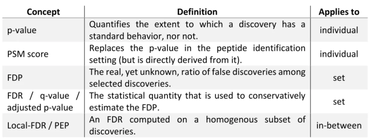
Table 2: Summary of the concepts reviewed in this article
Concept Definition Applies to
p-value Quantifies the extent to which a discovery has a
standard behavior, nor not. individual
PSM score Replaces the p-value in the peptide identification
setting (but is directly derived from it). individual
FDP The real, yet unknown, ratio of false discoveries among
selected discoveries. set
FDR / q-value / adjusted p-value
The statistical quantity that is used to conservatively
estimate the FDP. set
Local-FDR / PEP An FDR computed on a homogenous subset of
discoveries. in-between
Contributions
17
Acknowledgment
The author acknowledges financial support from “Agence Nationale de la Recherche”,``Infrastructures Nationales en Biologie et Santé'', and ``Investissements d'Avenir'' under grant numbers ANR-10-INBS-08 (ProFI project) and ANR-15-IDEX-02 (Life (is made of choice) Project). The author would also like to thank Quentin Giai Gianetto for fruitful discussions.
References
1. Serang, O.; Käll, L. Solution to statistical challenges in proteomics is more statistics, not less. Journal of proteome research
2015, 14(10), 4099-4103.
2. Kim, M. S.; Pinto, S. M.; Getnet, D.; Nirujogi, R. S.; Manda, S. S.; Chaerkady, R.; ...; Pandey, A. A draft map of the human proteome. Nature 2014, 509(7502), 575-581.
3. Wilhelm, M.; Schlegl, J.; Hahne, H.; Gholami, A. M.; Lieberenz, M.; Savitski, M. M.; …; Mathieson, T. Mass-spectrometry-based draft of the human proteome. Nature 2014, 509(7502), 582-587.
4. Giai Gianetto, Q.; Couté, Y.; Bruley, C.; Burger, T. Uses and misuses of the fudge factor in quantitative discovery proteomics. Proteomics 2016, 16, 1955-1960.
5. Tyanova, S.; Temu, T.; Sinitcyn, P.; Carlson, A.; Hein, M. Y.; Geiger, T.; ...; Cox, J. The Perseus computational platform for comprehensive analysis of (prote) omics data. Nature methods 2016, 13(9), 731-740.
6. Larsson, O.; Wahlestedt, C.; Timmons, J. A. Considerations when using the significance analysis of microarrays (SAM) algorithm. BMC bioinformatics 2005, 6(1), 129.
7. Deutsch, E. W.; Overall, C. M.; Van Eyk, J. E.; Baker, M. S.; Paik, Y. K.; Weintraub, S. T.; Lane, L.; Martens, L.; Vandenbrouck, Y.; Kusebauch, U.; Hancock, W. S.; Hermjakob, H.; Aebersold, R.; Moritz, R. L.; Omenn, G. S. Human proteome project mass spectrometry data interpretation guidelines 2.1. Journal of Proteome Research 2016, 15, 3961-3970.
8. Gigerenzer, G. Mindless statistics. The Journal of Socio-Economics 2004, 33(5), 587-606. 9. Trafimow, D. Marks, M. Editorial. Basic and Applied Social Psychology 2015, 37(1), 1-2.
10. Käll, L.; Storey, J. D.; MacCoss, M. J.; Noble, W. S. Assigning significance to peptides identified by tandem mass spectrometry using decoy databases. Journal of proteome research 2008, 7(01), 29-34.
11. Nesvizhskii, A. I. A survey of computational methods and error rate estimation procedures for peptide and protein identification in shotgun proteomics. Journal of proteomics 2010, 73(11), 2092-2123.
12. The, M.; Tasnim, A.; Käll, L. How to talk about protein‐level false discovery rates in shotgun proteomics. Proteomics
2016, 16(18), 2461-2469.
13. Cohen, J. The Earth Is Round (p<. 05). American Psychologist 1995, 50(12), 1103.
14. Giai Gianetto, Q.; Combes, F.; Ramus, C.; Bruley, C.; Couté, Y.; Burger, T. Calibration plot for proteomics: A graphical tool to visually check the assumptions underlying FDR control in quantitative experiments. Proteomics 2016, 16(1), 29-32. 15. Ramus, C.; Hovasse, A.; Marcellin, M.; Hesse, A. M.; Mouton-Barbosa, E.; Bouyssié, D.; ...; Garin, J. Benchmarking
quantitative label-free LC–MS data processing workflows using a complex spiked proteomic standard dataset. Journal of
Proteomics 2016, 132, 51-62.
16. Efron, B. Large-scale inference: empirical Bayes methods for estimation, testing, and prediction (Vol. 1). Cambridge University Press 2012.
17. Hochberg, Y.; Benjamini, Y. More powerful procedures for multiple significance testing. Statistics in medicine 1990, 9(7), 811-818.
18. Benjamini, Y.; Hochberg, Y. Controlling the false discovery rate: a practical and powerful approach to multiple testing. Journal of the royal statistical society. Series B (Methodological) 1995, 289-300.
19. Benjamini, Y.; Yekutieli, D. The control of the false discovery rate in multiple testing under dependency. Annals of
statistics 2001, 1165-1188.
20. Benjamini, Y.; Krieger, A. M.; Yekutieli, D. Adaptive linear step-up procedures that control the false discovery rate. Biometrika 2006, 93(3), 491-507.
21. Tusher, V. G.; Tibshirani, R.; Chu, G. Significance analysis of microarrays applied to the ionizing radiation response. Proceedings of the National Academy of Sciences 2001, 98(9), 5116-5121.
22. Efron, B.; Tibshirani, R.; Storey, J. D.; Tusher, V. Empirical Bayes analysis of a microarray experiment. Journal of the American statistical association 2001, 96(456), 1151-1160.
23. Storey, J. D. A direct approach to false discovery rates. Journal of the Royal Statistical Society: Series B (Statistical
Methodology) 2002, 64(3), 479-498.
24. Storey, J. D.; Tibshirani, R. Statistical significance for genomewide studies. Proceedings of the National Academy of
Sciences 2003, 100(16), 9440-9445.
25. Storey, J. D.; Taylor, J. E.; Siegmund, D. Strong control, conservative point estimation and simultaneous conservative consistency of false discovery rates: a unified approach. Journal of the Royal Statistical Society: Series B (Statistical
18
26. Keich, U.; Noble, W. S. On the importance of well-calibrated scores for identifying shotgun proteomics spectra. Journal
of proteome research 2014, 14(2), 1147-1160.
27. Goeman, J. J.; Solari, A. Multiple hypothesis testing in genomics. Statistics in medicine 2014, 33(11), 1946-1978. 28. Keller, A.; Nesvizhskii, A. I.; Kolker, E.; Aebersold, R. Empirical statistical model to estimate the accuracy of peptide
identifications made by MS/MS and database search. Analytical chemistry 2002, 74(20), 5383-5392.
29. Gupta, N.; Bandeira, N.; Keich, U.; Pevzner, P. A. Target-decoy approach and false discovery rate: when things may go wrong. Journal of the American Society for Mass Spectrometry 2011, 22(7), 1111-1120.
30. Elias, J. E.; Gygi, S. P. Target-decoy search strategy for increased confidence in large-scale protein identifications by mass spectrometry. Nature methods 2007, 4(3), 207-214.
31. Levitsky, L. I.; Ivanov, M. V.; Lobas, A. A.; Gorshkov, M. V. (2016). Unbiased False Discovery Rate Estimation for Shotgun Proteomics Based on the Target-Decoy Approach. Journal of Proteome Research 2016, 16(2), 393-397.
32. Keich, U.; Kertesz-Farkas, A.; Noble, W. S. Improved false discovery rate estimation procedure for shotgun proteomics. Journal of proteome research 2015, 14(8), 3148-3161.
33. Käll, L.; Storey, J. D.; MacCoss, M. J.; Noble, W. S. Posterior error probabilities and false discovery rates: two sides of the same coin. Journal of proteome research 2007, 7(01), 40-44.
34. Käll, L.; Storey, J. D.; Noble, W. S. Non-parametric estimation of posterior error probabilities associated with peptides identified by tandem mass spectrometry. Bioinformatics 2008, 24(16), i42-i48.
35. Käll, L.; Storey, J. D.; Noble, W. S. QVALITY: non-parametric estimation of q-values and posterior error probabilities. Bioinformatics 2009, 25(7), 964-966.
36. Reiter, L.; Claassen, M.; Schrimpf, S. P.; Jovanovic, M.; Schmidt, A.; Buhmann, J. M.; ...; Aebersold, R. Protein identification false discovery rates for very large proteomics data sets generated by tandem mass spectrometry. Molecular Cellular Proteomics 2009, 8(11), 2405-2417.
37. Pham, T. V.; Piersma, S. R.; Warmoes, M.; Jimenez, C. R. On the beta-binomial model for analysis of spectral count data in label-free tandem mass spectrometry-based proteomics. Bioinformatics 2009, 26(3), 363-369.
38. Lazar, C.; Gatto, L.; Ferro, M.; Bruley, C.; Burger, T. Accounting for the Multiple Natures of Missing Values in Label-Free Quantitative Proteomics Data Sets to Compare Imputation Strategies. Journal of proteome research 2016, 15(4), 1116-1125.
39. Robin, X.; Turck, N.; Hainard, A.; Tiberti, N.; Lisacek, F.; Sanchez, J. C.; Müller, M. pROC: an open-source package for R and S+ to analyze and compare ROC curves. BMC bioinformatics 2011, 12(1), 77.
40. Käll, L.; Canterbury, J. D.; Weston, J.; Noble, W. S.; MacCoss, M. J. Semi-supervised learning for peptide identification from shotgun proteomics datasets. Nature methods 2007, 4(11), 923-925.