Dynamic Toll Pricing using Dynamic Traffic
Assignment System with Online Calibration
The MIT Faculty has made this article openly available. Please share how this access benefits you. Your story matters.Citation Zhang, Yundi, Bilge Atasoy, Arun Akkinepally, and Moshe Ben-Akiva. “Dynamic Toll Pricing Using Dynamic Traffic Assignment System with Online Calibration.” Transportation Research Record: Journal of the Transportation Research Board 2673, 10 (October 2019): 532– 46.
As Published http://dx.doi.org/10.1177/0361198119850135
Publisher SAGE Publications
Version Original manuscript
Citable link https://hdl.handle.net/1721.1/125430
Terms of Use Creative Commons Attribution-Noncommercial-Share Alike Detailed Terms http://creativecommons.org/licenses/by-nc-sa/4.0/
DYNAMIC TOLL PRICING USING DTA SYSTEM WITH ONLINE CALIBRATION 1 2 3 4 Yundi Zhang 5
Massachusetts Institute of Technology 6
Department of Civil and Environmental Engineering 7
77 Massachusetts Avenue, Room 1-249, Cambridge, MA 02139, USA 8 Email: [email protected] 9 10 Bilge Atasoy 11
Delft University of Technology 12
Department of Maritime Transport and Technology 13
Mekelweg 2, 2628 CD, Delft, The Netherlands 14 Email: [email protected] 15 16 Arun Akkinepally 17
Massachusetts Institute of Technology 18
Department of Civil and Environmental Engineering 19
77 Massachusetts Avenue, Room 1-178, Cambridge, MA 02139, USA 20 Email: [email protected] 21 22 Moshe Ben-Akiva 23
Massachusetts Institute of Technology 24
Department of Civil and Environmental Engineering 25
77 Massachusetts Avenue, Room 1-175, Cambridge, MA 02139 26
Email: [email protected] 27
28 29
Word count: 6,740 words text + 2 table x 250 words (each) = 7,240 words 30 31 32 33 34 35 36
Submission Date: August 1, 2018 37
ABSTRACT 1
We develop a toll pricing methodology using a dynamic traffic assignment (DTA) system. This 2
methodology relies on the DTA system’s capability to understand and predict traffic conditions, 3
thus we apply enhanced online calibration methodologies to the DTA system, featuring a heuristic 4
technic to calibrate supply parameters online. We develop improved offline calibration techniqus 5
in order to apply toll pricing in a real network consisting of managed lanes and general purpose 6
lanes. We test our online calibration methodologies using real data from this network, and find the 7
DTA system able to estimate and predict traffic flow and speed with satisfactory accuracy under 8
congestion. Toll pricing is formulated as an optimization problem to maximize toll revenue, 9
subject to network conditions and tolling regulations. Travelers are assumed to make route choice 10
based on offline calibrated discrete choice models. We apply toll optimization in a closed-loop 11
evaluation framework where a microscopic simulator is used to mimic the real network. Online 12
calibration of the DTA system is enabled to ensure good optimization performance. We tested toll 13
optimization under multiple experimental scenarios, and find our methodology is able to increase 14
toll revenue compared to when online calibration is not available. It should be noted the toll rates 15
and revenues presented in this paper are obtained in a simulation environment based on our 16
calibration and optimization algorithms, and as the work is undergoing these results are far from 17
being a recommendation to the managed lane operator. 18
19 20
Keywords: traffic networks, dynamic traffic assignment, online calibration, generalized least
21
squares, simultaneous calibration, managed lanes, dynamic pricing, toll optimization 22
INTRODUCTION 1
Congestion management aims to improve transportation system performance and reduce traffic 2
congestion by either altering traffic demand or changing transportation supply. Among congestion 3
management schemes, road pricing (i.e., tolling) is a commonly used strategy, which may aim to 4
generate revenue to recover road construction and maintenance cost thus incentivize improvement 5
to transportation supply, as well as managing congestion by altering temporal and spatial 6
dimensions of travel behaviors, decisions on mode choice, or whether to travel (1). 7
Among road pricing strategies, dynamic pricing has been extensively studied in recent 8
years (2). Applications of dynamic pricing arise in many cities. We believe in two criteria for an 9
effective dynamic pricing scheme: real-time efficiency and proactive decision making. 10
Computation time of any algorithm should be short enough to support real-time decision making. 11
Decisions should be made based on predicted traffic conditions instead of observed ones. 12
In this paper, we implement and test a dynamic toll pricing framework, where decisions 13
on toll are made in real time (every 5 minutes) based on predicted traffic conditions. We apply the 14
framework in the context of managed lanes and from the viewpoint of the operator with an 15
objective to maximize revenue while offering premium level of service. State estimation and 16
prediction are provided by a DTA system, DynaMIT. Travelers’ route choice behaviors are 17
predicted by discrete choice models based on travel time savings and toll rates. Toll optimization is 18
fully integrated with DynaMIT to maximize revenue subject to network conditions given tolling 19
regulations. The impact of toll optimization is evaluated through a closed-loop evaluation 20
framework so the platform optimizing the tolls is different from where the tolls are implemented 21
and evaluated. A microscopic simulator, MITSIM (3), is used as the second simulation platform 22
for evaluating the tolls, and it serves as the real world in this closed-loop framework. 23
Effective toll optimization is only possible when the DTA system is capable of 24
understanding and predicting current and future traffic conditions. We propose and apply a 25
heuristic online calibration method to calibrate supply parameters and reduce discrepancies in 26
sensor speed between simulation and actual data. We also apply generalized least squares to 27
calibrate OD demand. Performance of the online calibration methodology is tested by calibrating 28
DynaMIT towards real dataavailable for the case study of managed lanes in Texas. DynaMIT is 29
then deployed in the closed-loop setting to test toll optimization, and the online calibration module 30
calibrates DynaMIT towards simulated sensor measurements provided by MITSIM. 31
The effectiveness of the toll optimization can only be confirmed when the demand and 32
travel behaviors are represented accurately in the simulation platforms. In this paper offline 33
calibration of the microscopic simulator is also briefly discussed. It is calibrated to the real data 34
before deployment of the closed-loop framework. 35
Contributions of this study include proposal, implementation and testing of a heuristic 36
online calibration method for supply parameters with complexity of O(n) where n represents 37
number of segments in the network. Note the algorithm is parallelizable, and it works 38
simultaneously with existing generalized least squares (GLS) algorithm for OD calibration. 39
Secondly, we implement the enhanced dynamic toll pricing framework and test it under multiple 40
scenarios in a closed-loop testing framework. These tests show added benefit to toll optimization 41
due to online calibration. 42
The subsequent sections of this paper include a literature review on offline and online 43
calibration of traffic simulators, as well as congestion pricing strategies and applications. Then we 44
present the optimization framework, calibration methodologies, and close-loop evaluation 45
framework. Finally, we show the results on online calibration and toll optimization in a case study 46
with data from real network, followed by conclusions and future research directions. 47
LITERATURE REVIEWS 1
Earlier literatures on toll pricing often rely on simplified representation of supply and/or demand. 2
Pricing strategies are mostly reactive instead of proactive, without explicitly predicting traveler 3
behaviors in reaction to pricing strategies. Yin et al. (4) propose dynamic toll pricing approaches in 4
the context of managed lanes with the objective to maximize throughput. A feedback control 5
approach is applied, such that toll decisions are reactive to traffic conditions. 6
Recent literature on toll pricing includes studies applying proactive pricing strategies. 7
Jang et al. (5) propose a closed-form model to predict certain system performance measures and 8
tolling decisions are based on the predicted performance. Dong et al. (6) study the benefits of a 9
proactive control strategy where predictions play a role when adjusting tolls based on the deviation 10
from the desired network conditions, and their optimization is integrated into a DTA system 11
DYNASMART. With an attempt to simplify optimization, Chen et al. (7) develop a family of 12
surrogate-based models for optimization of dynamic tolls, i.e. optimization of a peak and off-peak 13
toll. They use a DTA system DynusT for constructing various surrogate models, and apply them to 14
a corridor in Maryland with a composite objective function of travel time, throughput and revenue. 15
For a simulation-based proactive toll pricing system, online calibration of the simulator is 16
important to ensure simulation accurately mimics the real network and toll pricing decisions are 17
made based on accurate prediction of traffic conditions. Online calibration of a DTA system 18
usually includes calibration of OD demand parameters, behavior parameters, and supply 19
parameters. Generalized least squares (GLS) is widely used for OD calibration. An iterative 20
calibration framework to jointly calibrate OD, behavioral and supply parameters in a mesoscopic 21
DTA model is studied by (4). The OD demand is calibrated by the GLS method, while behavior 22
and supply parameters are estimated with specific empirical methods. 23
Hashemi and Abdelghany (8) propose online calibration methods in a traffic management 24
context, using GLS for OD and an empirical methods for supply parameters. Hashemi and 25
Abdelghany then (9) apply these online calibration methods to support traffic management 26
strategy generations. They use a DTA system and a meta-heuristic search algorithm to generate 27
control strategies, and apply their model to a corridor in Dallas, with an objective to reduce total 28
travel time. Their optimization system predicts significant time savings with the optimal strategies 29
generated by it, but the actual impacts of such strategies are not tested in the real network or in a 30
simulation environment that is different from the DTA system itself. Yang et al. (3) develop a 31
microscopic traffic simulator MITSIM and propose a close-loop testing framework in which 32
traffic management strategies are implemented in the simulator and the performance of such 33
strategies are then evaluated. Lu et al. (10) propose a weight-SPSA algorithm to calibrate a 34
microscopic traffic simulator in order to ensure it is a good representation of the real world. 35
Recent advancements in online calibration methods include simultaneous calibration of 36
all parameters with the same model, and the extended Kalman filter (EKF) is an example. 37
Antoniou et al. (11) propose EKF for online calibration of DynaMIT. By linearizing the relation 38
between all measurements including speed and all parameters including supply parameters, the 39
EKF algorithm can be used to simultaneously calibrate all parameters towards all measurements. 40
More recently there have been research on large scale problems. Guptaet al. (12) develop 41
toll optimization method with generic algorithm based on prediction from DynaMIT, and apply the 42
model to Singapore expressway network, where 13 tolls are optimized. Zhang et al. (13) develop a 43
metamodel that embeds an analytical model of how calibration parameter is related to the 44
objective function. The methodology addresses calibration of OD demand and is demonstrated 45
with a case study of Berlin metropolitan area network. Prakash et al. (14) apply a principle 46
components approach to conduct online calibration using the GLS algorithm. By calibrating 47
principle components of parameters instead of original parameters, this method greatly scales 1
down the computation effort of large-scale online calibration problems. It slightly worsens 2
estimation accuracy but reaches better prediction accuracy, since principle components capture 3
inherent correlations of the parameters while removing noise. Prakash et al. (15) apply this 4
approach to online calibration using the EKF algorithm and obtain similar results, which implies a 5
potential of reducing dimensionality in large scale demand-supply simultaneous online calibration 6
problems 7
The toll pricing framework in this paper is a real-time proactive system where the toll 8
rates is optimized every 5 minutes based on predicted traffic conditions in the next 15 minutes. The 9
proof-of-concept has been demonstrated before on a toy network in Wang et al. (16), and this paper 10
enhances the methodology by integrating online calibration into the framework to achieve better 11
toll optimization performance in a case study of managed lanes in Texas. 12
13 14
METHODOLOGY 15
Overview of Toll Optimization Framework 16
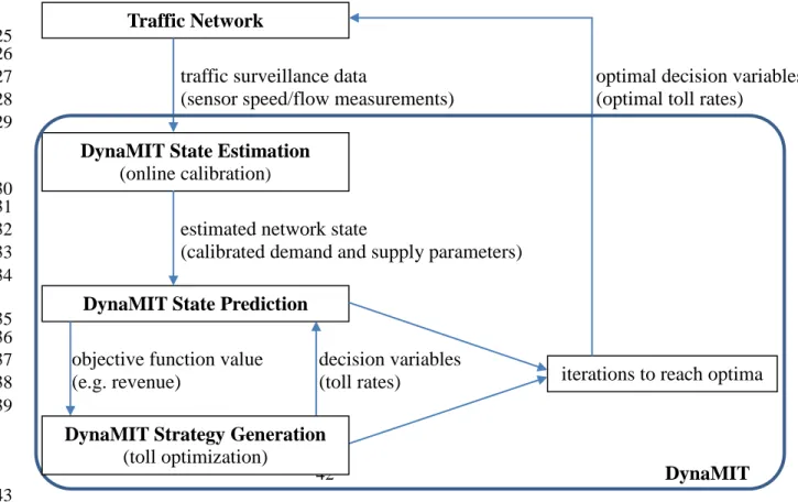
The toll optimization framework (16) is deployed with DynaMIT (17), a mesoscopic DTA system 17
developed in the ITS Lab of MIT. DynaMIT reads sensor data, calibrates its parameters to estimate 18
traffic state, and generate control strategies (toll rates) based on predicted traffic conditions 19
(Figure 1). Toll optimization is based on rolling horizon framework, i.e., for each rolling period
20
(e.g. 5 minutes), it receives new real-time information from the network, runs the estimation and 21
optimization modules, and provides optimized toll rates for the prediction interval (e.g. 15 22
minutes) to the network. 23
24 25 26
traffic surveillance data optimal decision variables 27
(sensor speed/flow measurements) (optimal toll rates) 28
29
30 31
estimated network state 32
(calibrated demand and supply parameters) 33
34 35 36
objective function value decision variables 37
(e.g. revenue) (toll rates) 38 39 40 41 DynaMIT 42 43 44
FIGURE 1 Toll optimization framework
45
Traffic Network
DynaMIT State Estimation
(online calibration)
DynaMIT State Prediction
iterations to reach optima
DynaMIT Strategy Generation
Optimization Formulation 1
The toll for each tolling location i is represented by 𝜃𝜃𝑖𝑖 = (𝜃𝜃𝑖𝑖1, ..., 𝜃𝜃𝑖𝑖𝑖𝑖), where T is the 2
number of tolling intervals in the optimization horizon. The speed and flow for each tolling 3
location i and tolling interval t are denoted by υit and qit, respectively. 4
The managed lane operator has to comply with tolling regulations, which need to be taken 5
care of by the optimization model. There is a toll cap per mile and the operator may decide to 6
exceed this toll cap, only under certain conditions. Specifically, given average speed (𝜐𝜐̅) and 7
volume (𝑞𝑞�) across all sensor locations and predefined critical values of speed (𝜐𝜐𝑐𝑐𝑐𝑐) and volume 8
(𝑞𝑞𝑐𝑐𝑐𝑐), the following rules are in effect: 9
• If 𝜐𝜐̅ ≤ 𝜐𝜐𝑐𝑐𝑐𝑐, toll rate is multiplied by a flexible demand factor between a lower bound
10
DFitlb and an upper bound DFitub, and the toll rate will increase compared to the previous
11
toll, i.e., DFitlb ≥ 1. 12
• If 𝑞𝑞� > 𝑞𝑞𝑐𝑐𝑐𝑐, depending on the level of 𝑞𝑞�, there is a set of rules to calculate a fixed demand
13
factor which may result with an increased, decreased or maintained toll value. 14
When either rule is adopted, the managed lanes are operated in mandatory mode. 15
The optimization model therefore includes a binary decision (𝛿𝛿𝑖𝑖𝑖𝑖) of switching or not to 16
the mandatory mode in addition to the decision on the toll vector (𝜽𝜽). The problem is formulated as 17 follows: 18 𝐦𝐦𝐦𝐦𝐦𝐦 ∑ ∑𝒊𝒊∈𝑰𝑰 𝒊𝒊∈𝑻𝑻𝒒𝒒𝒊𝒊𝒊𝒊𝜽𝜽𝒊𝒊𝒊𝒊+ 𝜶𝜶𝒊𝒊𝒊𝒊𝝊𝝊 𝐦𝐦𝐦𝐦𝐦𝐦(𝝊𝝊𝒊𝒊𝒊𝒊− 𝝊𝝊𝒄𝒄𝒄𝒄, 𝟎𝟎) + 𝜶𝜶𝒊𝒊𝒊𝒊𝒒𝒒𝐦𝐦𝐦𝐦𝐦𝐦 (𝒒𝒒𝒊𝒊𝒄𝒄𝒄𝒄− 𝒒𝒒𝒊𝒊𝒊𝒊, 𝟎𝟎) (1) 19 s.t. (νit, qit) = DTA(𝜃𝜃) ∀𝑖𝑖 ∈ 𝐼𝐼, 𝑡𝑡 ∈ 𝑇𝑇 (2) 20 δit ≤ 𝜂𝜂𝑖𝑖𝑖𝑖 ∀𝑖𝑖 ∈ 𝐼𝐼, 𝑡𝑡 ∈ 𝑇𝑇 (3) 21 δit ≥ 𝑀𝑀�𝛿𝛿𝑖𝑖(𝑖𝑖−1)− 1� + (1/100)(𝜃𝜃𝑖𝑖(𝑖𝑖−1)− 𝜃𝜃𝑖𝑖𝐶𝐶𝐶𝐶𝐶𝐶) ∀𝑖𝑖 ∈ 𝐼𝐼, 𝑡𝑡 ∈ 𝑇𝑇 (4) 22 �DFitlb, 𝐷𝐷𝐹𝐹𝑖𝑖𝑖𝑖𝑢𝑢𝑢𝑢, 𝜂𝜂𝑖𝑖𝑖𝑖� = 𝑓𝑓(𝜐𝜐𝑖𝑖𝑖𝑖, 𝑞𝑞𝑖𝑖𝑖𝑖) ∀𝑖𝑖 ∈ 𝐼𝐼, 𝑡𝑡 ∈ {2, … , 𝑇𝑇} (5) 23 δit𝜃𝜃𝑖𝑖(𝑖𝑖−1)𝐷𝐷𝐹𝐹𝑖𝑖𝑖𝑖𝑙𝑙𝑢𝑢 ≤ 𝜃𝜃𝑖𝑖𝑖𝑖 ≤ (1 − 𝛿𝛿𝑖𝑖𝑖𝑖)𝜃𝜃𝑖𝑖𝐶𝐶𝐶𝐶𝐶𝐶+ 𝛿𝛿𝑖𝑖𝑖𝑖𝜃𝜃𝑖𝑖(𝑖𝑖−1)𝐷𝐷𝐹𝐹𝑖𝑖𝑖𝑖𝑢𝑢𝑢𝑢 ∀𝑖𝑖 ∈ 𝐼𝐼, 𝑡𝑡 ∈ 𝑇𝑇 (6) 24 𝜃𝜃𝑖𝑖(𝑖𝑖−1)− 𝛥𝛥 − 𝛿𝛿𝑖𝑖𝑖𝑖𝑀𝑀 ≤ 𝜃𝜃𝑖𝑖𝑖𝑖 ≤ 𝜃𝜃𝑖𝑖(𝑖𝑖−1)+ 𝛥𝛥 + 𝛿𝛿𝑖𝑖𝑖𝑖𝑀𝑀 ∀𝑖𝑖 ∈ 𝐼𝐼, 𝑡𝑡 ∈ 𝑇𝑇 (7) 25 𝛿𝛿𝑖𝑖𝑖𝑖 ∈ (0,1) ∀𝑖𝑖 ∈ 𝐼𝐼, 𝑡𝑡 ∈ 𝑇𝑇 (8) 26 𝜃𝜃𝑖𝑖𝑖𝑖 ≥ 0 ∀𝑖𝑖 ∈ 𝐼𝐼, 𝑡𝑡 ∈ 𝑇𝑇 (9) 27
The objective function (1) has three terms: toll revenue and two penalty terms to account for 28
critical speed and volume pre-specified by the regulations. Namely, the second term is the penalty 29
for going below the critical speed and the last term is the penalty for exceeding the critical volume 30
on the managed lane. The critical speed is the same across the network, however the critical flow 31
changes based on the number of lanes. In this study, we decided to formulate these constraints 32
through penalty terms since we have a simulation-based setting. Namely, we cannot constrain the 33
simulator not to give certain speed and flow measurements, instead we evaluate the solution 34
through the resulting measurements based on if and how much it violates the desired conditions. 35
Furthermore, the penalty coefficients 𝛼𝛼𝑖𝑖𝑖𝑖𝜐𝜐 and 𝛼𝛼𝑖𝑖𝑖𝑖𝑞𝑞were set empirically. 36
Constraints (2) ensure that the predicted speed and volume are provided by traffic 37
simulator to evaluate the objective function and also for the decisions in future intervals. 38
Constraints (3) maintain that the system cannot enter mandatory mode (δ cannot be 1) if not 39
allowed by measurements (for the next interval) or predictions (for future intervals). Constraints 40
(4) enable a gradual decrease in the toll when exiting the mandatory mode. If the system was in 41
mandatory mode in t-1 and the toll was above the toll cap, the system needs to stay in mandatory 42
mode. If the conditions are getting better, the demand factors from the regulations will go down 43
and the toll will gradually decrease. 44
Constraints (5) maintain matching between the predicted traffic conditions and the 45
demand factors and the allowance to enter mandatory mode for the future intervals through 46
predetermined functions. Note that ηit is input for the next interval based on field measurements 1
and a variable to be optimized for the subsequent intervals based on predicted traffic state. 2
Similarly, DFitlb and DF𝑖𝑖𝑖𝑖𝑢𝑢𝑢𝑢are inputs for the immediate next interval and variables for the 3
subsequent intervals. DFitlb and DF𝑖𝑖𝑖𝑖𝑢𝑢𝑢𝑢 will be the same in the mandatory mode so that the toll will 4
be equal to the demand factor times the previous toll. On the other hand, when in dynamic mode, 5
DFitlb will be zero and DF 𝑖𝑖𝑖𝑖
𝑢𝑢𝑢𝑢 will be the toll cap. Constraints (6) regulate these bounds on the toll
6
such that if the decision is to stay in dynamic mode (δ=0), then the toll is optimized between 0 and 7
toll cap, otherwise (δ=1) toll rates follow the regulations in mandatory mode. 8
Finally, constraints (7) control the maximum change in the toll. This constraint is active 9
only in dynamic mode (δ=0), and not in mandatory mode (δ=1). Constraints (8)-(9) define the 10
decision variables as binary and nonnegative continuous, respectively. Currently this problem is 11
solved with simple search heuristics and future work involves other solution algorithms. 12
13
Calibration and Prediction in the DTA System 14
Effective control strategies rely on the DTA system’s capability to predict traffic conditions under 15
candidate toll rates. Prediction accuracy depends on state estimation performance. Offline and 16
online calibration are essential to ensure accurate estimation of the current network state. 17
A state is a vector consisting of demand and supply parameters. State estimation is the 18
real-time process of incorporating an initial state, historical data and real-time surveillance data to 19
achieve a more reliable estimation of the current state. 20
Offline calibration provides a priori values of the parameters which are then calibrated 21
online. For this research, we relied on IPF to obtain a historical time-dependent OD demand table 22
based on historical sensor flow measurements. We calibrated choice parameters empirically so that 23
simulated choice ratios matched actual data. For supply parameters, we have a closed-form model 24
which is described in next section, so we could estimate the model parameters with actual sensor 25
data. 26
For online calibration, GLS algorithm is used to estimate OD demand from real-time 27
sensor flow measurements. For supply parameters, we proposed a heuristic online calibration 28
framework to adjust supply parameters in real-time, and resulting simulation results matches 29
sensor data with satisfactory accuracy in terms of speed measurements, including when congestion 30
is present. 31
State prediction module predicts future states based on current state, taking into 32
consideration any historical information, strategies (e.g., future toll rates) to be deployed and 33
travelers’ response to guidance information. We formulate the prediction model as an 34
autoregressive process (11): 35
𝑥𝑥𝑖𝑖𝑝𝑝𝑐𝑐𝑝𝑝𝑝𝑝 − 𝑥𝑥𝑖𝑖ℎ𝑖𝑖𝑖𝑖𝑖𝑖 = ∑𝑛𝑛𝑖𝑖=1𝑓𝑓𝑖𝑖(𝑥𝑥𝑖𝑖−𝑖𝑖𝑝𝑝𝑖𝑖𝑖𝑖− 𝑥𝑥𝑖𝑖−𝑖𝑖ℎ𝑖𝑖𝑖𝑖𝑖𝑖)
36
where 𝑥𝑥𝑖𝑖𝑝𝑝𝑐𝑐𝑝𝑝𝑝𝑝 is predicted parameter value for current interval; 37
𝑥𝑥𝑖𝑖ℎ𝑖𝑖𝑖𝑖𝑖𝑖 is historical parameter value for current interval;
38
𝑛𝑛 is the autoregressive degree; 39
𝑓𝑓𝑖𝑖 is the autoregressive coefficient for degree i;
40
𝑥𝑥𝑖𝑖−𝑖𝑖𝑝𝑝𝑖𝑖𝑖𝑖 is estimated parameter value for the i-th interval ahead;
41
𝑥𝑥𝑖𝑖−𝑖𝑖ℎ𝑖𝑖𝑖𝑖𝑖𝑖 is historical parameter value for the i-th interval ahead.
42
For demand, we estimate 𝑛𝑛 and 𝑓𝑓𝑖𝑖 using offline calibrated time-dependent OD parameters. For 43
supply, since we do not obtain time-dependent supply parameters offline, the above autoregressive 44 model is simplified as 45 𝑥𝑥𝑖𝑖𝑝𝑝𝑐𝑐𝑝𝑝𝑝𝑝 − 𝑥𝑥ℎ𝑖𝑖𝑖𝑖𝑖𝑖 = 𝑓𝑓(𝑥𝑥 𝑖𝑖−1𝑝𝑝𝑖𝑖𝑖𝑖 − 𝑥𝑥ℎ𝑖𝑖𝑖𝑖𝑖𝑖) 46
and the coefficient 𝑓𝑓 is empirically determined. We then use the predicted parameters 𝑥𝑥𝑖𝑖𝑝𝑝𝑐𝑐𝑝𝑝𝑝𝑝 as 1
input to simulate traffic for the prediction interval (e.g. 15 minutes) and obtain predicted sensor 2
measurements. 3
To evaluate the calibration and prediction accuracies, we use RMSN (Root Mean Square 4
error, Normalized) to quantify the difference between actual and simulated measurements (11). 5
RMSN is defined by the following equation: 6 𝑅𝑅𝑀𝑀𝑅𝑅𝑅𝑅 = �𝑀𝑀1∑ (𝑦𝑦𝑖𝑖𝑝𝑝𝑖𝑖𝑖𝑖− 𝑦𝑦 𝑖𝑖𝑖𝑖𝑐𝑐𝑢𝑢𝑝𝑝)2 𝑀𝑀 𝑖𝑖=1 𝑦𝑦��������𝚤𝚤𝑖𝑖𝑐𝑐𝑢𝑢𝑝𝑝 7
where 𝑀𝑀 is the number of measurements; 8
𝑦𝑦𝑖𝑖𝑝𝑝𝑖𝑖𝑖𝑖 is the estimated value of the i-th measurement;
9
𝑦𝑦𝑖𝑖𝑖𝑖𝑐𝑐𝑢𝑢𝑝𝑝 is the true value of the i-th measurement.
10 11
Algorithm for Online Calibration of Supply Parameters 12
The optimization module of this study relies heavily on accurate prediction of drivers’ choice 13
between Managed Lanes and General Purpose Lanes, and travel speed or travel time would be an 14
important factor for their decisions. Therefore, it is essential to make sure the state estimation 15
module could accurately reveal the supply parameters thus simulated travel speed could match 16
actual sensor speed measurements. 17
18 19
(for each road segment) 20
21
sensor flow sensor speed & flow
22 23 24
sensor speed & density 25
26 27
if sudden drop of speed if sudden dissipation of congestion 28
not captured by simulator not captured by simulator 29
30 31 32
estimated OD estimated supply parameters
33 34 35
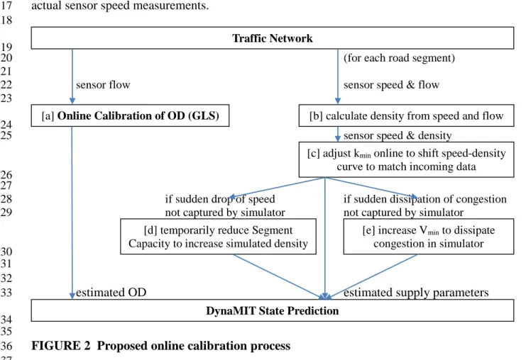
FIGURE 2 Proposed online calibration process 36
37
In DynaMIT traffic simulation module, a road segment consists of queuing part 38
(downstream) and moving part (upstream) (17). Queue would form only if flow on the segment 39
exceeds Segment Capacity, or queue on downstream segment spills out. Traffic speed on the 40
queuing part is subject to a queuing model. If a queuing part does not exist, or it does not occupy 41
the full segment, then traffic speed on the moving part is described by the following relationships: 42
Traffic Network
[a] Online Calibration of OD (GLS) [b] calculate density from speed and flow
[c] adjust kmin online to shift speed-density curve to match incoming data
[d] temporarily reduce Segment Capacity to increase simulated density
[e] increase Vmin to dissipate congestion in simulator
𝑣𝑣 = max (𝑣𝑣𝑚𝑚𝑖𝑖𝑛𝑛, 𝑣𝑣𝑖𝑖) 1 𝑣𝑣𝑖𝑖 = 𝑣𝑣𝑚𝑚𝑚𝑚𝑚𝑚 when k ≤ 𝑘𝑘𝑚𝑚𝑖𝑖𝑛𝑛 2 𝑣𝑣𝑖𝑖 = 𝑣𝑣𝑚𝑚𝑚𝑚𝑚𝑚�1 − �𝑘𝑘−𝑘𝑘𝑘𝑘 𝑚𝑚𝑚𝑚𝑚𝑚 𝑗𝑗𝑗𝑗𝑚𝑚 � 𝛽𝛽 � 𝛼𝛼 when k > 𝑘𝑘𝑚𝑚𝑖𝑖𝑛𝑛 3
where k is density, 𝑣𝑣 is speed, 𝑣𝑣𝑖𝑖 is an intermediate variable, and the other 6 parameters 4
(𝑣𝑣𝑚𝑚𝑖𝑖𝑛𝑛, 𝑣𝑣𝑚𝑚𝑚𝑚𝑚𝑚, 𝑘𝑘𝑚𝑚𝑖𝑖𝑛𝑛, 𝑘𝑘𝑗𝑗𝑚𝑚𝑚𝑚, 𝛼𝛼, 𝛽𝛽) as well as Segment Capacity are referred to as supply parameters in 5
DynaMIT. 6
For each road segment, there are 7 supply parameters and we estimated their a priori 7
values from speed and flow measurement data offline. When deploying real-time toll optimization, 8
we adjust a selection of supply parameters online in reaction to real-time sensor measurements. 9
Figure 2 illustrate the specific operations. Step [b] ~ [e] constitute the heuristic online calibration
10
method for supply parameters. Note that step [d] or [e] are only used in rare cases to correct 11
simulation errors. 12
13
Closed-loop Evaluation Framework 14
Before the toll optimization framework is implemented in the real world, the validity and 15
performance of the developed models and algorithms need to be tested in a simulation 16
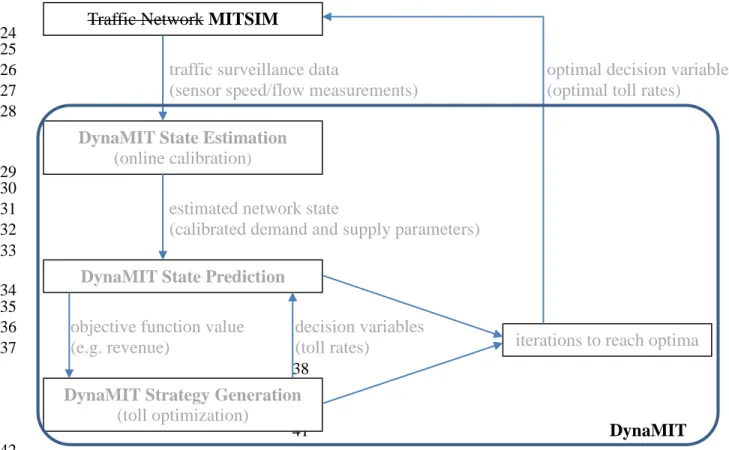
environment. Therefore, a closed-loop evaluation framework is applied by using a microscopic 17
simulator as a representation of the actual traffic network (Figure 3). 18
In this study we used MITSIM as the testbed. MITSIM is a microscopic traffic simulator 19
developed in the ITS Lab of MIT (3). It incorporates road topography, time-dependent OD 20
demand, driving behavior (car following, lane changing, etc.) models and route choice models, 21
simulates individual vehicle’s movements and generates simulated sensor measurements. 22
23 24 25
traffic surveillance data optimal decision variables
26
(sensor speed/flow measurements) (optimal toll rates)
27 28
29 30
estimated network state
31
(calibrated demand and supply parameters)
32 33 34 35
objective function value decision variables
36
(e.g. revenue) (toll rates)
37 38 39 40 DynaMIT 41 42
FIGURE 3 Closed-loop evaluation framework
43
Traffic Network MITSIM
DynaMIT State Estimation
(online calibration)
DynaMIT State Prediction
DynaMIT Strategy Generation
(toll optimization)
Route choice is modeled as a path-size 1
logit model, which takes into account the 2
similarities between paths that are overlapping. 3
Drivers make route choice decisions based on 4
information on toll rates and travel times. To 5
mimic real-world, drivers are assumed to have 6
access to real-time traffic information, e.g. 7
through mobile navigation applications, so they 8
are aware of current traffic conditions (i.e., 9
travel time) on downstream links. As for toll 10
rates, they are assumed to know real-time toll 11
rates only when they are close to the decision 12
point. Otherwise, the drivers rely on historical 13
toll rates (at that time of day) to make decisions. 14
The optimized toll rates are 15
implemented in MITSIM, and DynaMIT is 16
provided data from sensors in MITSIM rather 17
than a real-world traffic surveillance system. 18
The closed-loop testing framework requires that 19
the microscopic traffic simulator represents the 20
real-world accurately, i.e., drivers in MITSIM 21
behave similarly to those in the real-world, and 22
demand-supply interactions occur in the same 23
way. This can be achieved by calibrating 24
MITSIM towards real data. 25
Calibration of the microscopic traffic 26
simulator relies on an enhanced W-SPSA 27
algorithm (18). Demand parameters and selected 28
behavior parameters are calibrated 29
simultaneously to minimize the discrepancies 30
between simulated and actual sensor 31 measurements. 32 33 34 CASE STUDY 35
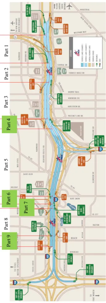
The methodologies are applied to the NTE 36
TEXpress network, a 13-mile corridor on I-820 37
and TX-183 with managed lanes (ML) and 38
general purpose lanes (GPL) (Figure 4). The 39
network is equipped with sensors that provide 40
traffic flow and speed measurements, and toll 41
gantries for non-stop tolling. 42
The private operator of this corridor 43
provided us with samples of data collected on 9 44
Fridays in summer 2017, which included sensor 45
flow and speed measurements, toll rates, and 46 AVI data. 47 Pa rt 1 Pa rt 2 Pa rt 3 Pa rt 4 Pa rt 5 Pa rt 7 Pa rt 6 Pa rt 8 Pa rt 9
The tolls are applied on two tolling segments. Segment 1 is highlighted darker in Figure 1
4, and segment 2 (upstream to segment 1) has lighter color. Toll gantries are located at the
2
beginning of each tolling segment, and at entry ramps to ML. A driver pays a toll when entering 3
ML. The toll rate is determined with respect to the entry point but not exit point. If the driver 4
continues from tolling segment 2 to segment 1 on westbound, he/she pays a second toll. 5
In this case study we focused on the westbound (WB) of the network. For ease of analysis, 6
the WB corridor is divided into 9 parts based on locations of entry and exit ramps on ML, as shown 7
on Figure 4. Part 1~4 belong to tolling segment 2, and Part 5~9 belong to tolling segment 1. 8
9
Offline Calibration 10
The AVI data gives an insight to the OD pattern but they only includes a fraction of vehicles. The 11
data are used as seed OD for better offline calibration. We use iterative proportional fitting (IPF) 12
algorithm to scale up the AVI-based OD, according to flow at origin and destination nodes. Flow 13
data are available at most origin and destination nodes, either obtained from sensors on 14
corresponding origin and destination links, or calculated from sensor flow on nearby links 15
according to the flow conservation law. The IPF algorithm converged with no more than 0.1% 16
error in terms of fitting origin or destination flow. 17
The route choice model in DynaMIT is a path-size logit model, where probability of 18
choosing path i is specified as 19
P(i) =∑eVi+lnPSieVj+lnPSj 𝑗𝑗∈𝐶𝐶
20
where C is the set of all possible paths, and PSi is the path size variable for path I, specifying the 21
path’s degree of overlapping with other paths. Vi is the systematic utility of path i, given by the 22
following equation: 23
Vi = − μ(TTi−VOTtolli+ 𝑐𝑐𝑖𝑖)
24
where μ is the scaling factor, TTi and tolli are travel time and toll cost on path i, VOT is the 25
driver’s specific value of time, and 𝑐𝑐𝑖𝑖 is a constant. We assume different drivers have different 26
VOT which is subject to a log-normal distribution. The choice model was estimated empirically to 27
make sure simulated choice ratios match actual data. For a successful calibration, we introduced 28
the constant term to capture some network-specific phenomena. We also allowed the model 29
parameters to be different in different periods, which includes morning (5:30-9:00), mid-day 30
(9:00-14:00), afternoon (14:00-18:00) and evening (18:00-21:00). These periods are determined 31
based on historical toll rates on the network. 32
We estimated supply parameters with Day 1 data. We firstly estimated a set of supply 33
parameters for each type of road segments (ML, GPL, ramp), and using the results as starting 34
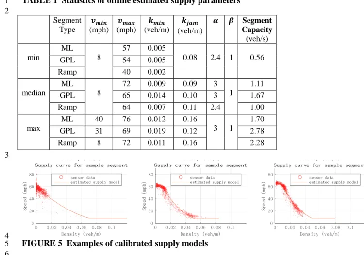
values, we estimated supply parameters for each road segment. The statistics of estimated supply 35
parameters are presented in Table 1. Figure 5 shows the data points and estimated supply curve for 36
a selected road segment. 37
After the offline calibration process, we obtain a set of parameters for Day 1, and the 38
simulation results have an error of 19% in RMSN for flow measurements and 15% for speed 39
measurements. 40
TABLE 1 Statistics of offline estimated supply parameters 1 2 Segment Type (mph) 𝒗𝒗𝒎𝒎𝒊𝒊𝒎𝒎 (mph) 𝒗𝒗𝒎𝒎𝒎𝒎𝒎𝒎 (veh/m) 𝒌𝒌𝒎𝒎𝒊𝒊𝒎𝒎 𝒌𝒌𝒋𝒋𝒎𝒎𝒎𝒎 (veh/m) 𝜶𝜶 𝜷𝜷 Segment Capacity (veh/s) min ML 8 57 0.005 0.08 2.4 1 0.56 GPL 54 0.005 Ramp 40 0.002 median ML 8 72 0.009 0.09 3 1 1.11 GPL 65 0.014 0.10 3 1.67 Ramp 64 0.007 0.11 2.4 1.00 max ML 40 76 0.012 0.16 3 1 1.70 GPL 31 69 0.019 0.12 2.78 Ramp 8 72 0.011 0.16 2.28 3 4
FIGURE 5 Examples of calibrated supply models 5
6 7
Online Calibration and Prediction 8
We calibrate DynaMIT offline to Day 1 data and obtain a set of parameters. Using Day 1 9
parameters as a priori values, we then calibrate DynaMIT online for the other 8 days. 10
For each 5-minute time interval, we first run a DynaMIT simulation with predicted 11
parameters from last interval, obtain simulated measurements, and then apply demand and supply 12
calibrations independently to obtain calibrated demand and supply parameters. Finally it simulated 13
the traffic with calibrated parameters. The GLS algorithm worked well for calibrating OD demand 14
parameters, as long as error of simulated speed was not large. The heuristic was effective to 15
replicate real-world congestions in the simulator. Results of online calibration are shown in Table 2 16
as OC demand&supply. The No OC case is a base case where historical OD and supply parameters 17
are used in the simulation. The OC demand only case has OD calibrated by GLS algorithm, but 18
historical supply parameters are used in simulation. 19
Taking Day 1 offline calibration results as baseline, simulation of other days had much 20
larger error for flow if online calibration was not performed, because those days had different 21
demand from Day 1. Error for speed was about the same, because supply parameters were static in 22
these cases and they are similar in different days. Online calibration of demand greatly improved 23
flow accuracy. Addition of supply online calibration then improved speed accuracy, due to its 24
capability to calibrate supply parameters dynamically. In all cases, prediction RMSNs are slightly 25
larger than estimation, which is as expected and acceptable, because the prediction model 26
incorporated additional errors. 27
TABLE 2 Online calibration and prediction accuracies 1
2
RMSN(%)
Estimation Prediction (0~15min later)
0~5min 5~10min 10~15min
Flow Speed Flow Speed Flow Speed Flow Speed Day 1 Offline calibration results 19 15
Day 2 No OC 22 16 22 15 22 15 22 15 OC demand only 12 16 16 15 19 15 19 15 OC demand&supply 12 13 17 11 19 12 22 12 Day 3 No OC 23 12 23 14 23 14 22 14 OC demand only 12 12 16 14 18 14 19 14 OC demand&supply 12 10 16 10 19 11 21 11 Day 4 No OC 23 13 23 15 23 15 23 15 OC demand only 12 13 16 15 18 15 19 15 OC demand&supply 13 11 17 11 19 12 22 12 Day 5 No OC 38 22 38 23 38 24 38 23 OC demand only 16 23 23 24 25 24 26 24 OC demand&supply 18 19 24 17 26 18 29 18 Day 6 No OC 33 17 33 14 33 14 33 14 OC demand only 13 17 19 14 22 14 23 14 OC demand&supply 15 15 21 10 23 11 25 12 Day 7 No OC 23 14 23 14 23 14 23 14 OC demand only 12 14 16 14 18 14 19 14 OC demand&supply 12 12 16 10 19 10 22 11 Day 8 No OC 23 12 24 13 24 13 24 13 OC demand only 14 12 18 13 20 13 21 13 OC demand&supply 14 10 19 10 21 10 23 10 Day 9 No OC 22 12 22 13 23 13 23 13 OC demand only 11 12 16 13 18 13 19 13 OC demand&supply 14 9 19 9 21 10 22 10 3
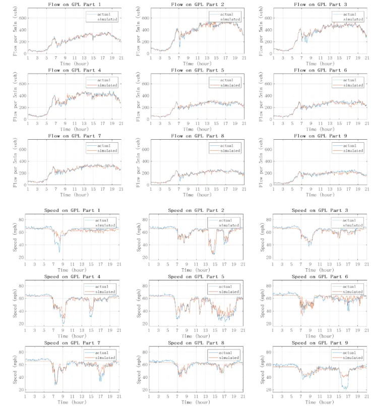
We present more detailed results for Day 6 in Figure 6. It shows the simulated flow and 4
speed after online calibration of demand and supply, compared with true measurements. Each 5
small plot shows average flow or speed on one of the nine parts of the GPL. 6
We can see the proposed online calibration methods were successful to replicate flow and 7
speed fluctuations in each part of the westbound GPL, despite in some cases simulated congestions 8
are still not as severe as actual data. ML has overall less congestion and their plots are omitted. 9
The results below demonstrate that we are capable of understanding and predicting traffic 10
conditions when congestions are present, the optimization module is conducted with accurate 11
evaluation of the objective function, and DTA system is able to make informed decisions on toll 12
rates. 13
1
2 3
FIGURE 6 Comparison of actual and simulated flow and speed 4
5 6
Toll Optimization 1
We evaluated the toll optimization framework in closed-loop. We firstly calibrate MITSIM 2
towards sensor measurements of Day 6, and RMSN of the calibration result was 19% for flow and 3
17% for speed. We then applied the toll optimization framework and implemented the optimized 4
toll rate in MITSIM. 5
We compare this toll rate with a base toll, which is obtained with the same toll 6
optimization methodologies, except that online calibration is not enabled. In such situation, 7
DynaMIT is fed with parameters that has been calibrated offline towards Day 1 data. Comparing 8
optimized toll with this base toll highlights the added benefit of online calibration in the 9
prediction-based dynamic tolling. 10
We observed higher toll revenue when evaluating optimized toll rates in closed-loop, 11
compared to base toll rates. We also evaluated the toll optimization framework under certain 12
experimental scenarios, and our experiments generated higher revenue in the simulation 13
environment. 14
There are 5 gantries on westbound of the network. The toll optimization model generates 15
toll rates for the 2 gantries located at the beginning of each tolling segment. Toll rate at each of the 16
other 3 gantries is a fraction of the gantry at the beginning of the corresponding tolling segment. 17
Per tolling regulations, the toll rate may change dynamically every 5 minutes, and the amount of 18
change cannot exceed ±$0.5. Toll rates on tolling segment 1 and 2 are subject to an upper bound of 19
$5.3 and $5.7 respectively, except when ML becomes congested. Besides, we added a constraint 20
that toll rates on the two tolling segments cannot be different by more than $1, which is for 21
practical considerations and is consistent with historical toll rate data. 22
For this study, we use a search algorithm that searches 3 toll values for each tolling 23
segment, i.e., reduce by $0.2, keep the same, or increase by $0.2. The algorithm then evaluates 24
objective function by calculating toll revenue in the next 15 minutes. Figure 7 shows the optimized 25
toll rates for each tolling segment compared to base toll, and per-5-minute revenue under these two 26
tolls. Note that the revenue shown are calculated from simulation results by MITSIM, our testbed 27
for evaluating the toll optimization framework. Figure 8 and Figure 9 show flow on ML and speed 28
on GPL, comparing our simulation results under optimized toll rates and under base toll rates. 29 30 31 32 33
FIGURE 7 Comparison of base and optimized toll rates and revenues 34
1 2
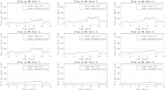
FIGURE 8 Flow on ML under base and optimized toll rates 3 4 5 6 7 8 9
FIGURE 9 Speed on GPL under base and optimized toll rates 10
Our optimization results suggest, in general, higher toll rates compared to the base toll except 1
during PM peak when they both reach the upper bound, because online calibration successfully 2
captures most congestions, and travelers’ route choice model in our system shows room for toll 3
increase under congestion. According to our simulation of 5:30-21:00 period in the closed-loop 4
framework, revenue is 8.1% higher under optimized toll rates. Under optimized toll, flow on ML is 5
generally lower when toll rate is higher, and thus speed on GPL gets lower. However, on tolling 6
segment 2 (Part 1~4) GPL becomes very congested after 17:00 that optimized toll rates maintained 7
at high levels even after the PM peak period. In addition, there is still higher flow on ML at Part 1, 8
which leads to much higher revenue during that period. This is due to bthe fact that our framework 9
is not addressing congestions on GPL. Based on our evaluation in the closed-loop framework, the 10
above results demonstrate that the dynamic toll pricing framework with the online calibration is 11
promising with improved revenue. 12
Flow on GPL is not shown because it’s complimentary to flow on ML. Speed on ML is 13
not shown because ML is generally not congested. With optimized toll rate, speed on ML is 14
maintained at a high level. Besides, we use different model parameter values in 4 periods of the 15
day, which leads to sudden change of simulated flow between periods. 16
Limitations includes a narrow search range for the toll rates. If the algorithm allows toll 17
rate to change by a higher value for each interval, the revenue under optimized toll rates might be 18
even higher. 19
20
Toll Optimization under Different Scenarios 21
We further evaluated toll optimization under some experimental scenarios: 22
1. Toll rates are not subject to an upper bound. 23
2. Demand is 20% lower. 24
3. Drivers’ braking behaviors are more conservative and deceleration rates are 50% lower. 25
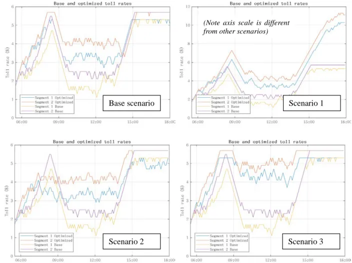
Optimized toll rates under these scenarios are presented in Figure 10. These experiments are done 26
for 5:30-18:00. 27
Under scenario 1, when upper bound on toll is not in effect, toll rates during AM and PM 28
peak periods would potentially increase to as high as twice the original upper bound, generating a 29
revenue gain of 5.3% during the simulation period of 5:30-18:00, which is a slightly larger gain 30
compared to 4.0%, the case where there is an upper bound. This indicates there is still room for 31
raising the toll rate above upper bound, based on travelers’ elasticity to toll as implied by our route 32
choice model. Nevertheless, the rate of increase reduces as the toll get higher since the response of 33
travelers is eventually effective and the supply-demand interaction is working under the proposed 34
framework. 35
Scenario 2 represents a day with 20% less demand, and optimized toll rates become lower 36
than the base scenario due to less congestion on GPL, but still higher than base toll during mid-day. 37
Since mid-day is not congested any way, reducing demand does not change optimized toll rate. 38
Toll revenue would be lower than base scenario because of less trips, but applying toll 39
optimization with online calibration still increase revenue by 1.7% compared to applying the base 40
toll rate that is not adjusted dynamically. 41
Scenario 3 simulates drivers driving in a more conservative way, potentially because of 42
bad weather. Due to slower deceleration rate, headway between vehicles has to increase, thus 43
overall capacity of the highway decreases. Due to more congestions, our toll optimization 44
algorithm chooses to maintain much higher toll rates compared to base case, and similar flow on 45
ML could be maintained, thus generates a revenue gain of 9.8% comparing to base toll rate. Under 46
heavier congestion drivers choose ML even when toll rates are much higher, due to larger saving in 47
travel time, on our proposed toll optimization framework benefits from online calibration to 1
estimate and predict congestions. 2
Above tests under the simulation environment demonstrate the important role of online 3
calibration in the prediction-based dynamic toll pricing framework. When online calibration is 4
enabled and we are able to estimate and predict traffic conditions with satisfactory accuracy, 5
decisions on toll rates made by the DTA-based optimization is better than the case when no online 6
calibration is available. The added benefit of online calibration is especially large when there is 7
significant congestion on the network, and is less evident when no congestion is present, which 8
confirms that online calibration of supply parameters in an effort to match simulated and actual 9
traffic speed is key to the success of the prediction-base tolling framework. 10
11
12
FIGURE 10 Optimized toll rates under base and experimental scenarios 13
14 15 16
Base scenario Scenario 1
Scenario 2 Scenario 3
(Note axis scale is different from other scenarios)
CONCLUSION 1
This paper presents calibration and optimization methodologies for a dynamic toll pricing 2
framework. This framework is integrated with a DTA system to optimize toll rates by evaluating 3
toll revenues under predicted traffic conditions. Thus online calibration is important to ensure the 4
DTA correctly understand and predict traffic conditions. We propose a heuristic online calibration 5
algorithm to dynamically adjust supply parameters in the DTA system in response to real-time 6
surveillance data. This algorithm is tested with real sensor data from a corridor consisting of 7
managed lanes and general purpose lanes, and the calibration accuracy is impressive, even when 8
significant congestion is present. With online calibration enabled, we test the toll optimization in a 9
closed-loop evaluation framework. A microscopic simulator is calibrated offline towards real data, 10
and integrated in the toll pricing framework as a representation of real network. The DTA-based 11
optimization framework generated optimized toll rates which are implemented in the microscopic 12
simulator instead of in real network. The closed-loop toll optimization test is done under a base 13
scenario and three experimental scenarios. In each scenario, optimized toll rates are consistent 14
with our prior belief, and higher toll revenue is obtained when optimized toll rates are 15
implemented, compared to the base toll rates generated in a system without online calibrations. We 16
also observerd the system is maintained to be real-time, i.e., the optimized tolls are always 17
obtained in less than 5 minutes. 18
It should be noted this research is conducted in a simulation environment relying on a 19
discrete choice model to predict travelers’ route choices under different traffic conditions and toll 20
rates, and parameters of that model are known to the DTA system optimizing the toll. Recent 21
research by Burris and Brady (19) suggests travelers’ route choice behaviors may be more complex 22
than a route choice model that only considers travel time and monetary cost. Further research is 23
necessary before we can claim our methodology being valid in real world. Future research includes 24
a comprehensive and personalized model for travelers’ decisions to use managed lanes, as well as 25
calibrating the choice model parameters online. 26
Future research on toll optimization algorithms may potentially improve the effectiveness 27
of toll optimization and obtain larger revenue gain, or it may be extended to incorporate other 28
objectives. Current algorithm is a simple search algorithm and should be improved without 29
sacrificing computational efficiency. Robust toll optimization algorithms may also be another 30
future direction to account for the situation that the DTA system may not have perfect knowledge 31
on predicted network conditions and travelers’ choice behaviors. 32
33 34
ACKNOWLEDGMENT 35
We acknowledge our sponsor Ferrovial/CINTRA, and acknowledge Ricardo Sanchez, Thu Hoang, 36
Andres De Los Rios, Megan Rhodes, John Brady, Ning Zhang, and Wei He for the help and 37
valuable feedbacks throughout the project. We are also grateful to our colleagues from MIT and 38
SMART for their help: Ravi Seshadri, Haizheng Zhang and Samarth Gupta. 39
40 41
AUTHOR CONTRIBUTIONS 42
The authors confirm contribution to the paper as follows: study conception and design: Y. Zhang, 43
A. Akkinepally, B. Atasoy, M. Ben-Akiva; data collection: Y. Zhang, B. Atasoy; analysis and 44
interpretation of results: Y. Zhang, A. Akkinepally, B. Atasoy; draft manuscript preparation: Y. 45
Zhang, B. Atasoy, A. Akkinepally. All authors reviewed the results and approved the final version 46
of the manuscript. 47
REFERENCES 1
1. Saleh, W. and Sammer, G., Travel Demand Management and Road User Pricing: 2
Success, Failure and Feasibility. Routledge, New York, 2009
3
2. de Palma, A. and Lindsey, R., 2011. Traffic congestion pricing methodologies and 4
technologies. Transportation Research Part C: Emerging Technologies, 19(6), 5
pp.1377-1399. 6
3. Yang, Q., Koutsopoulos, H. and Ben-Akiva, M., 2000. Simulation laboratory for 7
evaluating dynamic traffic management systems. Transportation Research Record: 8
Journal of the Transportation Research Board, (1710), pp.122-130.
9
4. Yin, Y. and Lou, Y., 2009. Dynamic tolling strategies for managed lanes. Journal of 10
Transportation Engineering, 135(2), pp.45-52.
11
5. Jang, K., Chung, K. and Yeo, H., 2014. A dynamic pricing strategy for high occupancy 12
toll lanes. Transportation Research Part A: Policy and Practice, 67, pp.69-80. 13
6. Dong, J., Mahmassani, H.S., Erdoğan, S. and Lu, C.C., 2011. State-dependent pricing for 14
real-time freeway management: Anticipatory versus reactive strategies. Transportation 15
Research Part C: Emerging Technologies, 19(4), pp.644-657.
16
7. Chen, X.M., Xiong, C., He, X., Zhu, Z. and Zhang, L., 2016. Time-of-day vehicle mileage 17
fees for congestion mitigation and revenue generation: A simulation-based optimization 18
method and its real-world application. Transportation Research Part C: Emerging 19
Technologies, 63, pp.71-95.
20
8. Hashemi, H. and Abdelghany, K., 2015. Integrated method for online calibration of 21
real-time traffic network management systems. Transportation Research Record: Journal 22
of the Transportation Research Board, (2528), pp.106-115.
23
9. Hashemi, H. and Abdelghany, K.F., 2016. Real-time traffic network state estimation and 24
prediction with decision support capabilities: Application to integrated corridor 25
management. Transportation Research Part C: Emerging Technologies, 73, pp.128-146. 26
10. Lu, L., Xu, Y., Antoniou, C. and Ben-Akiva, M., 2015. An enhanced SPSA algorithm for 27
the calibration of Dynamic Traffic Assignment models. Transportation Research Part C: 28
Emerging Technologies, 51, pp.149-166.
29
11. Antoniou, C., Ben-Akiva, M. and Koutsopoulos, H.N., 2007. Nonlinear Kalman filtering 30
algorithms for on-line calibration of dynamic traffic assignment models. IEEE 31
Transactions on Intelligent Transportation Systems, 8(4), pp.661-670.
32
12. Gupta, S., Seshadri, R., Atasoy, B., Pereira, F.C., Wang, S., Vu, V., Tan, G., Dong, W., Lu, 33
Y., Antoniou, C., Ben-Akiva, M. Real time optimization of network control strategies in 34
DynaMIT2.0. Paper presented at the Transportation Research Board 95th Annual 35
Meeting, 2016. 36
13. Zhang, C., Osorio, C. and Flötteröd, G., 2017. Efficient calibration techniques for 37
large-scale traffic simulators. Transportation Research Part B: Methodological, 97, 38
pp.214-239. 39
14. Prakash, A.A., Seshadri, R., Antoniou, C., Pereira, F.C. and Ben-Akiva, M.E., 2017. 40
Reducing the Dimension of Online Calibration in Dynamic Traffic Assignment Systems. 41
Transportation Research Record: Journal of the Transportation Research Board, (2667),
42
pp.96-107. 43
15. Prakash, A.A., Seshadri, R., Antoniou, C., Pereira, F. and Ben-Akiva, M., 2018. 44
Improving Scalability of Generic Online Calibration for Real-Time Dynamic Traffic 45
Assignment Systems. Accepted by Transportation Research Record: Journal of the 46
Transportation Research Board.
16. Wang, S., Atasoy, B., Ben-Akiva, M. Real-time Toll Optimization based on Predicted 1
Traffic Conditions. Paper presented at the Transportation Research Board 95th Annual 2
Meeting, 2016. 3
17. Ben-Akiva, M., Koutsopoulos, H. N., Antoniou, C., and Balakrishna, R., 2010. Traffic 4
simulation with DynaMIT. In Fundamentals of traffic simulation, pp. 363-398. Springer, 5
New York, 2010. 6
18. Zhang, Y., 2017. Exploration of Algorithms for Calibration and Optimization of 7
Transportation Networks, MSc Thesis, Massachusetts Institute of Technology. 8
19. Burris, M. W., & Brady, J. F., 2018. Unrevealed Preferences: Unexpected Traveler 9
Response to Pricing on Managed Lanes Accepted by Transportation Research Record: 10
Journal of the Transportation Research Board
11
View publication stats View publication stats