Dynamic scheduling of a two-class queue with setups

HUZO

.M414

/V3.

t-o

Dewey

WORKING

PAPER

ALFRED

P.

SLOAN

SCHOOL

OF

MANAGEMENT

Dynamic

Scheduling

of

a

Two-Class

Queue

with Setups

Martin

L

Reiman

Lawrence

M.

Wein

#3692-94-MSA

May

1994

MASSACHUSETTS

INSTITUTE

OF

TECHNOLOGY

50

MEMORIAL

DRIVE

CAMBRIDGE,

MASSACHUSETTS

02139

Dynamic

Scheduling

of

a

Two-Class

Queue

with Setups

Martin

I.

Reiman

Lawrence

M. Wein

M.I.T.

LIBRARiES

:'

JUN

2

1994

Dynamic

Scheduling

of

a

Two-Class

Queue

with Setups

Martin

I.

Reiman

AT&T

Bell Laboratories

Murray

Hill,

NJ

07974

Lawrence

M.

Wem

Sloan School of

Management,

M.I.T.

Cambridge,

MA

02139

ABSTRACT

We

analyze

two

scheduling

problems

for a

queueing system

with a single server

and two

cus-tomer

classes.

Each

class has its

own

renewal arrival process, general service timedistribution

and

holding cost rate. In the first problem, a setup cos* is incurred

when

the server switches

from one

class to the other,

and

the objective is to

minimize

the long run expected average

cost ofholding

customers and

incurring setups.

The

setup cost is replaced

by

a setup time in

the second problem,

where

the objective is to

minimize

the average holding cost.

By

assuming

that the

queueing

system

operates

under

standard

heavy

traffic conditions,

we

approximate

the

dynamic

scheduling

problems by

diffusion control problems. For

both

problems, considerable

insight is gained into the nature of the optimal policy,

and

the

computational

results

show

that the

proposed

scheduling policy is within several percent ofoptimalover a

broad

range of

problem

parameters.

We

consider

two

dynamic

scheduling

problems

for asingle server

queueing system

with

two

classes of customers. In

both

problems, each class possesses its

own

renewal arrival process, general service time distribution

and

holding cost rate,

and

the server incurs a setup

when

switching

from

one class to the other. In the setup cost problem, a setup cost is incurred

and

the objective is to

minimize

the long run expected average setup

and

holding cost. In the setup time problem, a

random

setup time is incurred

when

the server switches class,

and

the objective is to

minimize

the long run expected average holding cost. In

both

problems, the server has threeoptions at each point in time: servea

customer

from

the class that iscurrently

set up, switch to the other class (and

immediately

begin service in the setup cost problem), or

sit idle.

These

scheduling

problems

have

numerous

applications,

most

notably for

manufacturing

systems

and

polling systems in

computer communication

networks.

The

setup time

problem

is

more

realistic

than

the setup cost

problem

in

most

situations, but is also n^rre difficult to

analyze.

However,

thesetup cost

problem

is relevant for

some

manufacturing systems

because,

motivated

by

just-in-time (JIT) manufacturing,

many

facilities have internalized their setup

times; that is, they have essentially

ehminated

their setup times at the

expense

of incurring

significant material, labor

and/or

capital costs.

Although

many

studies have analyzed the

performance

of polling

systems

under

various

scheduling policies (see Takagi 1986,

Boxma

and

Takagi 1992

and

references therein), relatively few papers have considered the optimal scheduling of polling systems.

The

seminal

paper

in this research area is Hofri

and Ross

(1987),

who

analyze a two-class

system

with setup costs

and

times. Let c,

and

//, denote the holding cost rate

and

service rate, respectively, for class i customers.

When

_ci^i

=

_C2H2, they

show

that a double threshold policy,

where

the server serves each class until its

queue

is

exhausted

and

the length of the other

queue

achieves a certain threshold level, minimizes the cost of setups

and

holding customers,

under

both

the

discounted

and

average cost criteria.

Very

little is

known

about

the polling

problem

when

ciMi ¥" f2M2, aside

from

the fact that the class with the larger cfi index should

be

served to

exhaustion.

Several authors have studied the setup time

problem

in

which

more

than two

classes are present. Structural results for

symmetric systems

are derived by Liu,

Nain

and Towsley

(1991)

and

references therein.

Browne

and

Yechiali (1989) derive

quasi-dynamic

index policies,

which

allow the server to choose the sequence ofclasses to visit at the beginning of each cycle, that

minimize

or

maximize

the

mean

cycle length.

Boxma,

Levy

and Westrate

(1991) derive

an

efficient polling table (a

predetermined

fixed visit sequence) for

minimizing

the

mean

waiting cost.

Bertsimas

and

Xu

(1993) derive lower

bounds

and

construct static policies that

perform

close to the

bound

when

all classes have identical c/i indices.

Van Oyen

and

Duenyas

(1992)

develop a

dynamic

scheduling heuristic based

on myopic reward

rates;

Duenyas

and

Van

Oyen

(1993) also construct a

dynamic

policy for the setup cost problem.

Since the two-class

asymmetric problem

appearsto be analytically intractable,

heavy

traffic

approximations

are

employed

in

an

attempt

to

make

further

headway.

T'lat is,

we

make

the heavy traffic

assumption

that the server

must

be

busy

the great majority ofthe

time

to satisfy

demand.

In thesetup cost problem,

we

also need to

assume

that the setupcosts are very large, roughly

two

orders of

magnitude

larger

than

the holding cost rate. Following in the tradition of Foschini (1977)

and

Harrison (1988),

we

study the diffusion control

problem

that arises as a

heavy

traffic

Hmit

of a sequence of

queueing

scheduling problems.

These

limiting control

problems

tend to

be

more

tractable

than

their

queueing

counterparts

and

have led to

network

scheduling policies (see, for example, Harrison

and

Wein

1990

and

Wein

1990b) that

have

a surprisingly simple

form and appear

to

perform

well.

Using

the

heavy

traffic averaging principle derived in

Coffman,

Puhalskii

and

Reiman

(1993),

we show

in Section 1 that the setup cost

problem

simplifies rather dramatically in the limiting

heavy

traffic regime: the

dimension

of the state space collapses

from

three (queue length ofeach clciss

and

the position of the server) to

one

(total workload).

This

result also

allows our analysis to naturally

decompose

onto

two

different time scales.

On

the very fast time scale over

which

individual

queue

lengths change,

we

myopically optimize a control that

specifiesthe

amount

oflowpriority

work

toserve as a function of thetotal workload.

This

state-dependent

control is derived in closed

form

and

offers considerable insight.

On

the slower time

scale over

which

the total

workload

varies, a singular control

problem

is solved that specifies a

busy/idle pohcy.

The

solution to this control

problem

leads to a rather

complex

equation for

one

variable,

which

represents a threshold level, that can easily be solved numerically.

The

setup time

problem

is addressed in Section 2,

and

the averaging principle in

Coffman,

Puhalskii

and Reiman

(1994) leadsto a limiting control

problem

that again isone-dimensional, although here

we

obtain

an

explicit diffusion control problem.

The

control,

which

represents the

amount

oflowpriority

work

toserve as a function of the total workload,

appears

inthe drift

term

ofthe diffusion process in a nonlinear fashion,

and

consequently the

optimahty

equation

leads to a nonlinear ordinary differential equation

(ODE)

that

cannot be

solved explicitly.

However,

we

use asymptotics to obtain a scheduling policy; the asymptotics also reveal a

substantial qualitative difference

between

the optimalpolicies in the setupcost

and

setup time cases.

For

both

problems,

we

use the value iteration algorithm to obtain "exact"

optimal

policies foravarietyoftestcases,

and

show

inSection 3 that thesuboptimalityofthe

proposed

policies is within several percent ofoptimal over a

broad

range of

problem

parameters.

Our

presentation ofthe analysis,

and

indeed the analysis itself, is rather informal

through-out. For example,

we

do

not prove that the limiting control

problems

are the

heavy

traffic

limit ofa sequence of

queueing

scheduling problems. Also, several of our claims regarding the nature ofthe limiting control

problems

and

their optimal solutions are not proved. Providing

a rigorous presentation of our results

would

be extremely

demanding,

and would

take us far afield

from

our

two

main

objectives: to obtain

fundamental

insights into the nature of the

optimal

policies

and

to develop effective scheduling policies for these systems.

However,

much

ofour analysis relies

upon

observations that have

been

rigorously proven for simpler systems,

and

we

have

no

doubt

that our results are essentially correct.

We

hope

that this

approach

increases the accessility ofthe

paper

withoutsacrificing the persuasiveness ofour

arguments.

1

THE

SETUP COST

PROBLEM

1.1

Problem

Description

Customers

ofclass i

=

1,2 arrive according to

independent

renewal processes,

where

A,

and

c^j

denote

respectively the arrival rate

and squared

coefficient of variation (variance divided

by

the square of the

mean)

of the interarrival times.

Each

class has its

own

general service

time

distribution with service rate /Xj

and

squared

coefficient of variation c^j,

and

we

define the

system's traffic intensity

by

p

=

Yn=i{^i/f^i)-

A

cost c, is incurred per unit time for holding

a class i

customer

in the system.

A

setup cost

K/2

is

imposed

whenever

the server switches

from one

class to the other, so that A' is the setup cost per cycle.

The

server hcis three scheduling options at each point in time: serve the class that is

currently set up, switch to the other class

and

initiate service, or sit idle. Since a switchover

considered.

We

assume

that the server

works

in a

preemptive-resume

fashion, although the

heavy

traffic analysis is too crude to capture the effects ofthe

nonpreemptive

discipline as

an

alternative assumption. Let Qi{t) be the

number

ofclass i

customers

in

queue

or in service at time t,

and

let J{t) denote the

number

of times the server sets

up

in the time interval \0,t\.

Then

our objective is to find a nonanticipating (with respect to the

queue

length process)

scheduling policy to

minimize

limsup

—;E

r-.oo

T

rY,c,Q,{t)dt+^^J{T)

Jo

~1

^

(1.1)

1.2

The Heavy

Traffic

Normalizations

A

precise formulation ofthe

approximating

diffusion control

problem

requires

much

nota-tion that

would

not

be

subsequently used. In addition, the limiting control

problem

will not be explicitly solved; rather,

we

optimize over a specific

form

of policy that is introduced in Subsection 1.4.

Hence

the

heavy

traffic control

problem

will not be precisely formulated,

and

a description of the

heavy

traffic conditions

and

normalizations will suffice for our purposes.

The

approximating

control

problem

is the limit of a sequence ofscheduling

problems

in-dexed by

the

heavy

traffic scaling

parameter

n,

where

n

—> _oo. Since a

heavy

traffic limit

theorem

will not

be

proved here,

we

avoid unnecessary notation by considering a single large integer

n

satisfying y/n{l

—

p)

=

c,

where

c ispositive

and

of

moderate

size (that is, 0(1)); this

standard heavy

traffic condition requires the server to be

busy

the great majority of the time

over the long run.

As

we

willsee later, theschedulingpolicy that arises out ofour

heavy

traffic

analysis is

independent

ofthe

system parameter

n. Let V,

be

the unfinished workload process forclass i; Vi{t) isthe

amount

oftimea continuously

busy

server requires to clearalloftheclass

i

customers

who

are present in the

system

at time t.

The

normalized, or scaled,

queue

length

process is defined

by

Zj(i)

=

Qt{nt)/y/n- similarly, W,(t)

=

V't(ni)/v^ denotes the

normalized

workload

process.

We

approximate

these normalized processes

by

the appropriate,

and

yet to

be

defined, fimiting processes.

Although

Vi{t) is not directly observable

by

the scheduler at time i, the normalized

workload

process is

more

convenient to

employ than

the

normalised

queue

length process in the

approximating

heavy

traffic control problem.

However,

we

use the linear identity Zj

=

HiW^

to translate the solution of the

approximating

control

problem

into a scheduling policy that is expressed in

terms

ofthe original

queue

length _{process (Qi, Q2)-}

This

linear identity isjustified

by

extant

heavy

traffic limit

theorems

for

many

queueing

systems.

In addition to speeding

up

time

by

a factor of

n

and

reducing the

queue

lengths

by

a

factor of y/n,

we

also

need

to rescale the cost

parameters

C;

and

A'.

The

crux of

problem

(1.1) is the tradeoff

between

setup costs

and

holding costs,

and

hence to obtain a nontrivial solution to the

approximating

control problem, these

two

costs need to be of the

same

order

of

magnitude.

Since only the ratio of these

two

costs matters,

without

loss of generality

we

leave the holding cost rates ci

and

C2 unsealed at _0(1),

and

only scale the setup cost

K.

The

following

thought

experiment

allows us to conclude that the setup cost

K

needs to

be

divided

by n

in the

approximating

control problem.

The

heavy

traffic condition implies that there are

0(^/n) customers

in the original

queueing

system,

and hence 0(1)

scaled

customers

in the

heavy

traffic system.

The

holding cost rate is eff'ectively multiplied

by

n

because of the

time

scaUng, so holding costs are incurred in the limiting control

problem

at the rate of0{n^'^) per

unit time. Since

0{y/n) customers

are in the system, the server switches class every

0{\/n)

unsealed

time

units,

on

average, implying that setup costs are incurred at the rate of

0{^)

and

setup costs areincurred at rate0{y/n), the setup cost

K

must

be

0{n)

for these cost rates

to

be

ofthe

same

order,

and

to get

an 0(1) Hmiting

setup cost,

we

must

divide the setup cost

K

by

the

heavy

traffic

scahng parameter

n. Consequently, let k

= K/n

denote the normalized setup cost.

Thus, heavy

traffic conditions for the setup cost

problem imply

that the traffic

intensity should

be

near one

and

the setup cost should be large.

A

canonical

example

is to set

n

=

100

and

set c,ci,C2

and

k all equal to one, so that p

=

0.9

and

the setup cost A'

=

100.

1.3

A

Preliminary

Heavy

Traffic

Result

The

starting point for thesetup cost

problem

is arecent

heavy

traffic result

due

to

Coffman,

Puhalskii

and

Reiman

(1993),

which

will be referred to hereafterasthe

CPR

result.

We

present

an

informal statement ofa special case ofthis

heavy

traffic limit

theorem

that will suffice for our purposes.

As

in

problem

(1.1), consider a

queueing

system

with a single server

and

two

customer

classes.

The

CPR

result is derived

under

a specific

queue

discipline: the server serves

each class to exhaustion,

and

then switches class.

The

work

conserving nature ofthe disciphne

implies that the total

workload

process

W

=

Wi

+

W2

isidentical to the corresponding process

under

the

FCFS

policy. It follows

from

the

heavy

traffic

umit theorem

ofIglehart

and Whitt

(1970) that this process is well

approximated under heavy

traffic conditions

by

RBM(—

c, cr^),

which

is a reflected

Brownian

motion

(see Harrison 1985 for a definition)

on

[0,oc)

with

drift

—

c

and

variance

It turns out to

be

impossible to obtain a limit process for (M^i,

W2)

in the usualsense,

because

in the

heavy

traffic limit, the two-dimensional process

moves back

and

forth along the cross

diagonal at

an

infinite rate, the direction being

determined by

which

of the

two queues

is

being served; see Figure 1.

The

CPR

result provides

an

averaging principle that implies the following: given the

normahzed

total

workload

W

, the two-dimensional

workload

(H^i,W^2)

can be

treated as if it is uniformly distributed along the constant

workload

line

from

(0,

W)

to (ly, 0).

That

is, the two-dimensional distribution is

{UW,

(1

— U)W),

where

U

is a

uniform

[0,1]

random

variable that is

independent

of

W

.

This

averaging principle is

due

to a time scale decomposition.

On

the timescale giving rise

to reflected

Brownian

motion

for the total workload, the two-dimensional

workload

process

moves

(asymptotically) infinitely quickly. If

we

slow time

down

so that the two-dimensional

workload

moves

at a flnite

and

positive rate, the total

workload

stays fixed,

and

the

movement

of the two-dimensional

workload

is deterministic.

Although

this result has

been

proved only

under

the exhaustive policy,

we assume

that it holds

more

generally. This has far-reaching implications for the

heavy

traffic analysis ofour control problem. In particular, it allows us to

collapse the state space of the control

problem from

three dimensions (the

number

of

customers

ofeach class inthe

system and

the location of the server) to

one dimension

(the total workload).

1.4

The

Form

of the

Optimal

Policy

The

traditional

heavy

traffic

approach

to scheduling

problems

is to precisely formulate the

queueing

system

scheduling problem, find the limiting control

problem

that

approximates

the

scheduling

problem

\ni(lor

heavy

traffic conditions,

and

solve the latter problem.

The

approach

taken here is slightly different:

we

first argue that the optimal policy should be of a specific

form

in the

heavy

traffic limit,

and

then optimize the

approximating system

over this class of

(H^,0)

(1

-

U)W

serving

queue

1

W

=

Wi

+

W-, :

REM

W,

Figure 1:

The

heavy

traffic averaging principle of

Coffman,

Puhalskii

and

Reiman

(CPR).

Without

loss ofgenerahty,

we

assume

that ci/xi

>

c^fJ-j

and sometimes

refer to classes 1

and

2 as the high

and

lowpriority classes, respectively. Existing results (Hofri

and Ross

for Poisson arrivals

and

exponential service times,

and

Duenyas

and

Van Oyen

for Poisson arrivals

and

general service times) as well as intuition suggest that class 1 should

be

served to exhaustion.

(It is possible to construct

examples

where

this

pohcy

is not optimal.

Our

contention is that

it is asymptotically optimal in

heavy

traffic.)

When

the server is set

up

for class 1, the only

other decision is to specify

whether

the server should idle or switch to class 2

when

no

class 1

customers

are present. Since

we

work

with the normalized

workload

process (1^1,^2), theonly reasonable

form

ofthe optimal policy is to switch

when

W^jit)

>

W2

for

some

scaled threshold level ^2.

Since switching is instantaneous, Wi{t)

=

and

W2{t)

=

.r at the

moment

of switching,

where x

must

be greater

than

or equal to the threshold W2-

Because preemption

is allowed, the server should never idle at class 2

when

class 2

customers

are present.

The

CPR

result

implies that the total

workload

W

= Wi

+

W2

remains

constant in the

heavy

traffic time scale while the server is serving class 2 customers. Hence, our decision

can

be expressed as the

amount

u(x)

by which

the server depletes class 2's original work.

That

is, class 2 is served until

Wi{t)

=

u(.r)

and V^^IO

=

.r-u{x).

The

control u(x)

must be between

zero

and

x,

where

u

=

X

is the exhaustive policy. Figure 2 contains a picture with u{x)

=

.r/3 for a particular value of X. Since a different

amount

u can be chosen for each value of the total

workload

x,

the control u{x)

can

generate

any

possible switching curve in the nonnegative orthant,

and

so

is

without

loss ofgenerality.

W^

Figure 2:

The

control u{x)

=

x/3

for a fixed value of x.

the server

immediately

switches

back

to class 1

when

Wi{t)

=

u(x)

and W2{t)

=

x

-

u(x).

However,

if u(x)

=

x and

hence class 2 is served exhaustively, then the server

must

decide

whether

to idle or switch

back

to class 1.

Once

again, the obvious

form

ofthe optimal policy

in this case is to idle until Wi{t) is greater

than

or equal to wi. Notice that if the threshold levels wi

and

^2

were

both

zero, then infinite setup costs

would

be incurred.

In

summary,

the controls are the function u{x),

which

specifiesthe

amount

ofclass 2's

work

to serve,

and

the threshold levels

wi and

W2,

which

dictate the server's busy/idle policy.

The

form

of the optimal policy in

heavy

traffic is: serve class 1 until

Wi{t)

=

arid

W2{t)

>

u'2,' switch to class 2. If W2{t)

=

x

at the

moment

of switching, then serve class 2 until Wi{t)

=

u(x)

and

W2{t)

=

x

—

u{x). Ifu{x)

<

x, then switch to class 1; ifu{x)

=

x, then do not switch until

Wi{t)

>

vui.

1.5

An

Overview

of

the

Analysis

The

analysis hinges

on

the following crucial observation: since setups are instantaneous, the total workload process is only affected by the server's busy/idle policy, not by

how

often

the server switches class. Hence, the control u{x) only influencesthe total

workload

indirectly via the idling.

However,

u{x) does affect the rate at

which

holding costs

and

setup costs are

incurred

when

thetotal

workload

is x. Therefore, a two-step procedure is

employed

to find the

optimal

policy

{u{x),wi,W2)

within the specified form. In the first step, the control u{x) is

chosento

minimize

the cost rate for eachstate .r; this minimization is

performed

independently for each state x. In the second step,

we

attempt

to find the optimal threshold levels u)\

and

U'2,

and

L.Mice the optimal total

workload

process.

Our

heavy

traffic analysis will

show

that the

optimal

total

workload

process is a

RBM(—

c,o"'^)

_on

_[u;,oo),

_where

w

is a

parameter

that is chosen to

minimize

the total expected cost. Hence, the

Brownian model

is too

crude

to

distinguish

between

the

two

thresholds wi

and

W2,

and

so

we

set

both

«'i

and

»'2 equal to the

derived value of (/'.

As

in previous

heavy

traffic scheduling

work

(see Harrison 1988

and

Wein

19y0a, for ex-ample), the analysis naturally

decomposes

onto

two

time scales.

On

the very fast

time

scale,

where

individual ([ueues can

change

instantaneously fast,

we

myopically optimize over ii{x).

is solved to find the threshold, or reflecting barrier,

w

that specifies the busy/idle policy. 1.6

The

Optimal

u{x)

The

control u{x) is chosen to

minimize

the cost rate that is incurred

when

the normalized total

workload

process is x.

Under

the policy characterized

by

u(x), class 2's

work

is depleted

by

the

amount

u{x) if the total

workload

when

the server arrives to class 2 is x.

The

CPR

result implies that, forour purposes, it isas if

Wi

is uniformlydistributed

between

and

u{x),

and

W2

is uniformly distributed

between

x

-

u(i)

and

x. Since Zj

—

^jV^j, the holding cost rate

when

in state

x

is

V"

rrn/i "(^) ,

f2x-u{x)

2^

C^|I^E\VV^\

=

Cl/Xl— hC2M2 I '

Au(x)

, ,

=

C2M2-r

+

—

-

—

, (1-3)

where

A

=

ci/xi -C2/X2 (1-4)

To

find the setup cost rate

when

in state ;c,

we

need to find the cycle length. For a fixed total unfinished

workload

.r, the two-dimensional

workload

process (^1^1,^2)

moves back and

forth deterministically at

an

asymptotically infinite rate along the line

segment from

(0,x) to

((/(.r),x

-

u(x)); hence, the cycle length is deterministic.

We

determine

the deterministic cycle length,

and

hence the setup cost rate, as a function ofthe normalized

workload by

slowing

down

the time scale. Ifthe server finds

x

units of

work

in class 2

upon

arrival, then this

work

will

be

depleted at rate \

—

p^-

The

server

works

until 'W\[t)

=

u{x)

and

W2{t)

=

x

-

u(x),

which

occurs after u(x)/(l

-

_P2) time units.

As we

will

see later, the normalized total

workload

process

W

never

spends

any

time

below

max(it;i,«;2),

and

so

we

need

not include

any

unnecessary inserted idle time into the cycle lengthcalculation.

Therefore, it takes u(x)/{l

-

_p\) time units to deplete class 1

and complete

the cycle, resulting

in a cycle oflength u(.r)/(l

-

_P2)

+

u(x)/(l

—

p\). Since the holding costs are estimated using

a

heavy

traffic

approximation

and

the scheduling

problem

essentially trades offthe setup

and

holding costs, a

more

accurate analysis results if

we

assume

that p

=

1 in our cycle length

expression,

which

simplifies the cycle length to u{x)/pip2.

Because

two

setups are incurred in each cycle, the setup cost rate

when

in state

x

is pip2K/u{x).

Now

we

find the optimal u{x) by solving;

mm

C2P2-r

+

—

-

—

+

, , . (1-5)

u(x)e[o,x] 2 u(x)

If

we

define

2piP2K,

then straightforward calculus leads to

t/'(.r)

=

min(x,u;) . (!•")

Hence,

w

is the largest value of the total

workload

for

which

class 2 is served exhaustively.

Notice that

w

=

00

when

A

=

0,

and

so the optimal control in the balanced case is u*(.r)

=

.c

1.7

The

Optimal

Threshold

Level

In thissubsection,

we

analyze the normalized total

workload

process

under

the

form

of the

proposed

policy, using the control u*{x) in (1.7). This analysis

shows

that the total

workload

process

W

is a

RBM(—

c,a^)

on

[w,oo),

where

w

is a

parameter

that will be optimized over.

In the balanced case, the control u*{x) implies that the

form

of the optimal policy is to switch

from

class 1 to class 2

when

Wi{t)

=

and

W2{t)

>

W2,

and

switch

from

class 2 to

class 1

when

W2{t)

=

and

Wi{t)

>

u;i. Let us begin

by

assuming

that wi

<

W2-

When

the

two-dimensional

workload

process hits the point (x, 0),

where x 6

[wi,W2), then theserver will switch to class 1

and

the process instantaneously

moves

to the point (0,z). Since

x

<

W2, the server will not

immediately

switch

back

to class 2. Rather, the server serves

newly

arriving

class 1

customers

orsits idle until class 2's

workload

reaches W2- In the

heavy

traffic limit, time

is

sped

up

by

a factor of

n

and

the two-dimensional

workload

process instantaneously

moves

from

the point (0,x) to the point (0,^2)- Consequently, the total

workload

process never

spends

any time below

the value of u;2.

A

similar

argument

when

wi

>

u'2 implies that the

total

workload

process is a

RBM(—

c,a^)

on

[ma.x{wi, W2),00).

Thus,

the

heavy

traffic analysis

is too crude to distinguish

between

the thresholds

w\

and

W2,

and

we

follow the convention of setting

them

both

equal to w; later in this subsection, the cost

minimizing

value of

w

will

be

derived. Hence, the setup cost

problem decomposes

in the balanced case,

and

we

can

optimize

over a single threshold

parameter

w

independently of u*{x).

For the

imbalanced

case, the total

workload

process needs to

be

investigated

under

four

different cases,

depending

upon

the relative values of the normalized threshold levels u'i,W2

and

id.

Case

1:

<

wi,W2

<

w-

The

curves for switching

from

class 2 to class 1 for all four cases are pictured in Figure 3,

where

the vertical portion of the switching curve follows

from

(1.7).

The

argument

put forth in the balanced case implies that the total

workload

process in this

case is a

RBM(—

c, cr^)

on

[m.a.x{wi,W2),oo).

We

again set

wi and

IU2 equcd to the

parameter

w,

and

model

the optimal total

workload

process as a

RBM(—

c, cr^)

on

[u',00); in this case, the

parameter

w

is optimized over the region

<

w

<

w.

Case

2:

w <

wi,W2.

The

state (u'i,0) is never reached,

and

hence the

parameter wi

does not play a role here.

By

a similar

argument

as above,

W

is a

RBM(—

c, cr^)

on

[w2,oo).

Thus,

once

again,

we

set

wi

and

W2 equal to a

parameter

w, let

W

be

an

RBM(—

c, cr-)

on

[iti,c»),

and

optimize

w

over the region

w

>

w.

Case

3:

<

wj

<

w

<

102-

The

total

workload

W

is

an

RBM(-c,

a^)

on

[ii'2,00),

and

so

we

set

wi

and W2

equal to

w

and

optimize over

w >

w.

Thus,

case 3 reduces to case 2.

Case

4:

<

W2

<

w

<

wi.

The

parameter

wi is not a factor,

and

W

is

an

RBM(—

c,cr-)

on

[u,'2,oo). Hence, case 4 reduces to case 1.

In

summary,

it suffices to restrict our attention to cases 1

and

2; thus, as in the balanced

case, the single threshold

parameter

w >

can

be

optimized independently of u*{x).

Now

we

derive the optimal value of the

parameter

w. Substituting the

optimal

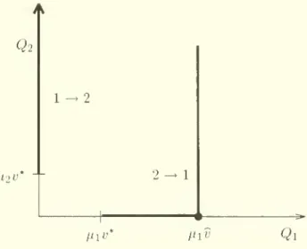
control

Case

1. li'i,u'2

< w

2 -^ 1

W9

"

-^

^•

Case

2.

w

<

wi, W2

W2

U^2 n

2^1

a

u'l v^i

Case

3. wi

<

w

<

W2^

W2

t 2

—

1

Wo

wi

w

W,

Case

4. W2

<

w <

wi

V2

1

+

^/2fHP2^

[

e-^^dxj

. (1.11)

Setting the derivative of the total expected cost with respect to

w

equal to zero yields

=

c(^l-(aw

+

l)e''^'"-'^'^)+apip2n(ae°'^{Ei{aw)-Ei{aw))~

-)

+

a^2pi/92A/ie"("'-'^)

+

C2fi2{aw

+

l)e"('"-'^) , (1.12)

or,

upon

simpUfication,

+

a'^pip.K.

(e^'^iEiiaw)

-

Ei{aw))

-

—]

, (1.13)

V

aw

J

where

E^{x)

=

/

—dt,

x>0

(1.14)

Jx t

is the exponential integral. It turns out that

C{w)

is not convex; however, the solution to (1.13) is well

behaved

numerically,

and

yields the global

minimum

of

C(w)

for the cases

we

consider.

We

denote this solution

by w*

and

refer to it as the optimal threshold level. Since

CK;e-°"'

+

piP2^

, (1-15)

it follows that the optimal total expected cost is

Cinj*)

=

Cw*

+

P^P^.

(1.16)

w*

In the balanced case

where

A

=

0, the first order condition (1.13) reduces to

—

-

e'''"

Ei{aw)

=

.5^^^ (1.17)

aw

a-pip2K

Moreover,

C"{w)

=

a^pxP2K (e^^'Eiiaw)

+

—^

-

—)

, (1.18)

V

(aw)-

aw

J

and

the convexity of

C{w)

follows

from

the

bound

e^Ei{x)

>

l/(x

+

1). Replacing e°""Ei{aiu)

by

its lower

bound

1/(001

+

1) in (1.17) gives a simple

approximate

expression for the

optimal

threshold level:

M

1 , /l ,

a-pip2K\

""-

=

_{a|^-2 +}

_Vi

+

_^:;]irj

• ^'-''^

1.8

The

Proposed

Scheduling

Policy

The

heavy

traffic solution is given

by

the control «*(.r) defined in (1.7),

which

specifics a

switching curve,

and

the threshold level w* satisfying (1.13) or (1.17).

We

use this solution to

propose

a scheduling policy in terms of the three-dimensional state of the original problem,

which

is the two-dimensional cjueue length process

(Qi.Qo), and

the server location. Since

both

u*{x)

and w*

are expressed in terms of the normalized

workload

W,

several steps are required to translate this

heavy

traffic solution into a

proposed

policy. First,

we

reverse the

heavy

traffic scaling to express the quantities «*(.r)

and

lu* in terms ofthe unsealed

workload

V. Since

W{t)

=

V{nt)/\/n,

when

the normalized

workload

W

equals x, then the original

workload

V

equals y,

where

y

=

^ynx.

The

control u*{x) requires the server to serve class 2 until

Wi

=

u*{x), or equivalently, until V'l/^/n

=

u*{y/y/n-). If

we

substitute A'/n for the

normalized setup cost k in (1.6), then

when

the total

workload

V

equals y, class 2 is served until

V]

=

\/nu

=

wninm

By

(1.20), class 2 is served exhaustively as long as the total

workload

V

is less

than

or equal

to

which, not surprisingly, ecjuals ^/nw. Similarly, if

we

define the unsealed threshold v*

=

\/nw*, then substitution of v/s/n. for w,

K/n

for k,,

and

2>/n(l

-

p)/a^ for

a

in (1.13)

and

(1.17) yields, respectively.

=

C

+

e''(

—

>(^v^^I^^A^-^i^

+

e-p,p2K

(^e'^E,{ev)

-

EiiOd))

-^)

(1.22)

and

^-e'^'E,{0v)

=

-^^,

(1.2.3) Bv

0^pip2K

where

. 2(1

_-p)

(1.24)

Similar substitutions into (1.19) gives

1/1

/I

«w^

,,^,,

„ _^ 2 _V 4 C1//1 I

Finally, the predicted optimal average cost for the original scheduling

problem

is

\/nC{w

)

=

Cv

H . (1-26)

V*

Noticethatthe quantitiesin (1.20)-(1.26) are independent ofthe heavy traffic scaling

parameter

n,

and

are expressed solely in terms of the primitive

problem

parameters.

Now

that the optimal control has

been

translated into unsealed workloads,

we

use the

simple

heavy

traffic relationship

_PiW^

=

Z,

between

workloads

and queue

lengths to exp'ess

the switching curve

and

thresholdlevel in termsof

queue

lengths.

The

only

remaining

hurdle is

that theresulting quantities are continuous,

whereas

the two-dimensional

queue

length process

resides

on

a lattice.

We

naively ignore this difference

between

our continuous solution

and

the discrete state space,

which

essentially

amounts

to

rounding

the threshold level

up

to the next

highest integer,

and rounding

the switching curve out to the next largest lattice points. In

addition to being the

most

natural translation of the continuous solution, it also prevents us

from rounding

a threshold level

down

to zero,

where

infinite setup costs

would be

incurred.

In the balanced case, the critical value v in (1.21) equals infinity,

which

corresponds to exhaustive service.

The

proposed

policy is:

when

Qi{t)

=

and

Q2{t)

>

112V*, then switch

from

class 1 to class 2;

when

Qiit)

=

and

Q\{t)

>

tx\v*, then switch

from

class 2 to class 1.

The

parameter

v* is the solution to (1.23). This policy is a special case of the double threshold

policy introduced by Hofri

and

Ross,

who

prove that the optimal policy is of this

form

in the

balanced case

when

arrivals are Poisson.

Q2

M21' 2 -^ 1

Ml"

Ml"

Qi

Figure 4:

The

proposed

scheduling policy

when

ci/ii

>

C2^i•2

By

(1.20), the

proposed

policy for the

imbalanced

case has a particularly simple form,

and

is pictured in Figure 4: -when Q\{t)

=

and

Q2{i)

>

M2^*i then sivitch

from

class 1 to class 2.

When

Q\{t)

>

^iv

or (Q2{t)

=

and

Qi(t)

>

ij,\v*), then switch

from

class 2 to class 1.

The

parameters

v

and

v* are defined in (1.21)

and

(1.22), respectively. Hence, the server

switches to the high priority class as

soon

as the

queue

length of that class

grows

to the level

Hiv.

By

(1.4)

and

(1.21), this critical level increases with the setup cost

K

and

decreases as the

c^

differential

between

the

two

classes gets larger.

Although

one

might

have expected a general nonlinear switching curve, the vertical

boundary

in Figure 4 is obtained. It is

worth

noting that the heuristic policy of

Duenyas

and

Van

Oyen

is also of this general form.

2

THE

SETUP TIME

PROBLEM

2.1

Problem

Description

The

only difference

between

thesetup time

problem

considered in thissection

and

the setup

cost

problem

is that a

random

setup time rather

than

asetup cost is incurred

when

the server

switches

from one

class to the other; all relevant notation

from

the setup cost

problem

will

be

retained.

By

CofFman,

Puhalskii

and

Reiman

(1994), the

performance

ofthis

system

in

heavy

traffic

depends

upon

the setup timedistributions only

through

tlie

mean

setup time per cycle,

which

we

denote

by

s.

The

server has three scheduling options at each point in time: serve a

customer from

the class that is currently set up, initiate a setup or sit idle.

The

objective is

to find a preemptive-resume, nonanticipating scheduling policy to

minimize

lim

sup

—

E

T—oo

T

T

2

(2.1)

2.2

The

Approximating

Diffusion

Control

Problem

Unlike, for example, the server vacation times in Kella

and

Whitt

(1990), the setup times are

not rescaled as the

heavy

traffic limit is approached; that is,

we

assume

that the setup times

are 0(1).

The

lack ofsetup costs has eliminated the incentive to insert unnecessary idleness

in

heavy

traffic; inserted idleness increases the workload,

which

in turn increases the holding costs. Hence, the

proposed

form

oftheoptimal policyissimpler

than

in the setupcost problem:

serve class 1 to exhaustion

and

then set

up

for class 2. If class 2's normalized unfinished

workload W-iit)

=

x

at the setup completion epoch, then serve class 2 until Wi{t)

—

u{x)

and

W2{t)

=

X

—

u{x),

and

immediately switch back to class 1.

As

in the setup cost problem, the control {u{x),x

>

0} can generate

any

arbitrary switching curve in the nonnegative orthant.

Sincethesetup times are 0(1), switchovers occur instantaneously in the

heavy

traffic limit.

Hence, the two-dimensional normalized unfinished

workload

process (M^i, VV2) will

move

at

an

asymptotically infinite rate

back

and

forth

between

(0,.z:)

and

(u(.r),x

—

u{x))

when

the total

normalized

workload

W

=

x, just as in the setup cost problem.

We

now

present a heuristic

argument

for the characterization of the normalized total unfinished

workload

process

W.

If

setup times are zero

and no

unnecessary idleness is inserted, recall that the the limiting process

is a

RBM

on

the nonnegative orthant with drift s/n{p

-

1)

and

variance a'- given

by

(1-2).

When

setup times are positive,

we

claim that the limiting process is a diffusion process

on

the nonnegative orthant with variance a^

and

a state-dependent drift,

which

we

denote /u(x').

Since the

system

is heavily congested, setups are incurred relatively rarely

and

the

mean

and

varianceofthesetup times

do

not

appear

in the variance

term

ofthe limiting diffusion process.

As

explained in Harrison

and

Nguyen

(1990), the drift ofthe stochastic process underlying a

heavy

traffic

approximation

ec}uals the expected

growth

rate of the normalized workload netfiowprocess,

which

is the arrival rate of

work minus

the potential (that is,

assuming

work

is always available) depletion rate ofwork.

With

zero setup times, unsealed

work

arrives at rate

p

and

is potentially depleted at rate one.

With

time

sped

up by

a factor of n

and workloads

reduced by

a factor of\/n, theexpected

growth

rateofthe normalized

workload

netfiow process

is \/n{p

—

1).

When

setup times are positive, the potential depletion rate of

work

is strictly

less

than one

and

will equal the fraction oftime that the server

spends

doing useful work; that

is, the fraction of time the server actually serves customers, rather

than

incurring setups.

We

claim that the drift

when

the normalized total

workload

is

x

equals

/x(.r)

=

y^(p-/(.T))

, (2.2)

where

/(.r) isthe fraction oftimethat the server

spends

doing useful

work

when

the normalized unfinished

workload

W

ecjuals x. Since cycles occur rapidly in

heavy

traffic, only averages

matter

and

we

can

carry out the calculation of f{x) over one cycle. Let us begin the cycle

when

all

y/nx

units of unsealed unfinished

work

V

is of class 2. Class 2

work

is depleted at

rate 1

-

p2 until V\{t)

=

^/nu{x)

and

V2{t)

—

\/n(x

-

u{x)),

which

takes y/nu{x)/{l

-

_P2) time

units. Similarly, y^u(:c)/(l

-

pi) time units are required to serve class 1 customers, thereby

completing

the cycle. Hence, if

we

assume

p

=

1 (see Section 1 for the rationale

behind

this assumption), then the length of the cycle is

\/nu(x) \/n.u(x)

^-^

₊

~

_-^

₊

_s,

(2.3)

P2 Pi

and

the fraction of time the server

spends

doing useful

work

is

fix)

=

\/nu{x) _. \/nu{x) P2 Pi Vnu(x) v/nM(x) ^ P2 P\ \/nu(x) ynu(.r)

+

spip2 ' (2.4)

By

(2.2), fi{x)

=

v/^(/9-l)

+

y^(l-/(x))

=

-c+v^(l-/(.r)).

(2.5) Since

rn

ti

w

Vnpip2S

PIP2S

V"(l

-

jyx))

=

_^

—

-—

as 71 -> oo , (2.6) ^/nu{x)

+

P1P2S u(x)

we

have H{x)

=

—-—-c.

(2.7) U[X)

In

summary, we

approximate

the normalized total unfinished

workload

process

W

by

a (p{x),a'^) diffusion. In the special case of exhaustive service (that is, u{x)

=

x

for all .r),

Coffman,

Puhalskii

and

Reiman

(1994)

show

that the normalized total unfinished

workload

process

weakly

converges to ^his diffusion process as p

—

> 1. If, in addition, c

=

(that is, p

=

1), this diffusion process is a Bessel process.

As

we

mentioned

earlier, given

W{t)

=

x, the two-dimensional process

(^1,^2)

behaves

the

same

with or

without

setup times; hence the holding cost rate

when

in state .r is given

by

(1.3). Therefore, the

approximating

diffusion control

problem

is to choose {u(-i')i-'''

^

0} ^^

minimize

limsup

—E

T—too

J-T

( ^^^^^ ,

Au(X(0)

a

C2P2X{t)

+

V^^

dt (2.8)

where

X

is a {p{x),a'^) diffusion process

and

u{x)

G

[0,x] for all

x

>

0.

The

previous literature

on heavy

traffic

approximations

of

queueing

scheduling

problems

assumes

zero setup times,

and

the time scale

decomposition

described in Section 1 leads to a

deterministic pathwise optimizationfor theoptimal

queue

length process

c^d

a singular control

problem

for the optimal cumulative idleness process.

The

presence of setup times destroys this simplifying structure,

and

(2.8) provides the first

example

of a scheduling

problem

for a

queueing

system

that is

approximated

in

heavy

traffic

by

a drift control problem.

2.3

Analysis

of

the

Diffusion

Control

Problem:

The

Balanced

Case

Problem

(2.8) simplifies considerably

when

each class has the

same

cp index. Setting

A

equal to zero in (2.8)

shows

that the

problem

reduces to choosing u{x) to

minimize

the

mean

of

the stationary distribution of the diffusion process A'. This goal is achieved by

minimizing

the

drift fi(x) in (2.7),

and

hence the optimal control is u{x)

=

x

for all x; therefore, the proposed

scheduling policy for the balanced case is to serve each class to exhaustion,

and

immediately

switch class.

The

resulting diffusion process is a Bessel process with

an

additive drift.

The

long run average cost of

any

stationary policy can be obtained

from

the stationary distribution (invariant measure) of the diffusion process 'induced' (via the resulting /i(x-)) by

the policy. Fortunately, the subject of stationary distributions of one dimensional diffusions

is old

and

well

understood

(c.f.

Mandl

1968, or

Karhn

and

Taylor 1981).

Given

a positive recurrent diffusion process

on

the nonnegative half line with drift //,(.r)

and

variance a^, the

stationary density satisfies the ordinary differential equation

(j^ d'^Txix) d , , , , ,,

Y^y-

-

^(/'(^)''^-'^))

=

°' •"

>

'^ (--^^

Associated with a reflecting

boundary

at zero, there is a

boundary

condition

a^ dTT{x)

~2

_Jx~

There

is also the normalization condition

=

/x(x)7r(x),

x-0.

(2.10)

oo

7r(.r)dx

=

1 . (2.11)

The

solution of (2.9)-(2.11) can be obtained using integrating factors. For the Bessel

process with

an

additive drift,

where

/x(x)

=

p\P2s/x

—

c, it can be

shown

by

a

bound

involving

Brownian

motion

that this process is positive recurrent

when

c

>

0.

The

solution of

(2.9)-(2.11) for this process is the

gamma

density

where

a

=

2c/cr^ is the scale

parameter and

/i

=

2pip2s/c^ is the

shape

parameter. (It is straightforward to verify that (2.12) solves (2.9), (2.10),

and

(2.11).

Standard

results

from

the theory ofordinary differential equations yield that (2.9)-(2.11) have a unique solution.) It

turns out that the Bessel process reaches the origin only if /3

<

1; if /3

>

1 the process will never reach zero.

The

solution (2.12) is valid for

both

of these cases.

Under

the exhaustive policy, the expected average cost incurred for the original

system

is \/n{c2P2

+

A/2)£'[A'(oo)],

where

A' is a {pip2s/x

—

c,a") diffusion. Since

rFlXI

.1

^C^

+

O

2p,p2S

+

a^ _,^^„,

7T-the

expected

average cost is

C{2pip2S

+

a'^) 2(1

_-p)

(2.14)

where

the cost

parameter

C

was

defined earlier as (cipi

+

C2^2)/2.

Forthebalanced case,

we

can alsointroducesetup costs into thesetup time

problem without

sacrificing tractability.

We

again let k

=

K/n

denote the normalized setup cost per cycle.

As

in the balanced case of the setup cost problem, the

proposed

policy is a double threshold policy

characterized

by

the

normahzed

threshold level w.

We

now

derive the optimal threshold value

under

the general

imbalanced

case, although thispolicy is only

proposed

forthe balancedcase.

Under

the threshold level lo, the diffusion process with drift fi{x)

=

pip2s/x

-

c

behaves

as before but isnot allowed to go

below

w.

The

stationary density 7r(x) ofthetruncated processis

obtained

by

solving equations analogous to (2.9), (2.10),

and

(2.11) with the reflecting barrier

at A'

—

lu.

The

solution,

which

yields the stationary density for the normalized

workload

W,

is ^(^)

=

_^^?TT^

for

x>«;,

• (2.15)

where

/•OO r(/?,a)

=

_/ t'^-^e-^dt (2.16)

is the incomplete

gamma

function.

Note

that (2.15) reduces to (2.12)

when

it)

=

0.

As

in the setup cost problem, setup costsare incurred at the rate p\p2i\./u(x)

when

W

=

x. Therefore, the expected setup cost per unit time is

Jw

1(13

+

I,

aw)

]

,/3+1^/3-i^-ax

r{/3,awj

l(p

+

l,Qu;)

r{p

+

l,aw)

p,P2aK

{aw)l'e--

\

where

the last

equahty

follows

from

the identity f3T{f3,

aw)

=

T{p

+

1,

aw) -

{aw)^

e~°'^.

The

expected holding cost per unit time is

C

_J^

X7r{x)dx,

where

/•OO

CV^"*"^

f^

/ X7:lx)dx

—

-

—

;

/ .c^"*"

e~^^dx

Ju_, ^ ' T{l5

+

l,aw)

Ju, r{(3

+

2,aw)

ar{l3

+

I,

aw)

a

r(p

+

I,

aw)

Hence, the expected total cost rate is

'g -aw

a[^^'^

TH3

+

l,aw)

r

P

V

FiP

+

^aw)^'

^'''''

If

we

define the constant k

=

pip2QK/

13, then it suffices to

minimize

{Cw -

K)(cvw)^e-""^

r(/?

+

l,m/;)

(2.20)

Using

the fact that

^r(/9

+

l,au;)

=

-ae

°'^{aw)^, considerable

manipulation

leads to the following first order optimality condition for lu*:

iau,Y>e-"

,

(,

_

AU

_^.

. (2.21)

r(/i+l,ouO

V

awj

a{K

— Cw)

Substituting v/y/ri. for w,

K/n

for k,

and

^lO

for

a

(see (1.24)) into (2.21) gives

=

_h

-

^

₊

7T7 W7-' ITTT-, (2-22)

r(^

+

1,^(0 V

Ov)

eipxpoOK

-

(3Cv

Although

we

have not

been

able to prove the existence ofa unique positive root v* to (2.22),

the numerical solution to this equation

was

well

behaved

for our test examples.

In

summary,

for the balanced case with setup times

and

setup costs,

we

propose

the

fol-lowing

scheduhng

policy for the original problem:

when

Qi{t)

=

and

Q2{t)

>

H2V*, switch

from

class 1 to class 2;

when

Q2{t)

—

and

Qi(t)

>

^i\v*. then switch

from

class 2 to class 1.

The

threshold v* is found by solving (2.22).

2.4

Analysis

of

the Diffusion

Control

Problem:

The

Imbalanced

Case

Notice that (2.8) is nonstandard, in the sense that the drift is

unbounded

at zero

and

will

be

unbounded

whenever

the control u{x)

=

0. Nonetheless,

we

proceed as if standard

arguments

apply (see, for example,

Mandl

1968),

and

write the

Hamilton-Jacobi-Bellman

optimality equation for

problem

(2.8) as

u{x)e[o,x]

[

2 V u{x) J 2

J

Hence, if

we

can find a constant g,

which

is referred to as the gain,

and

a potential (relative

value) function

V{x)

that solves (2.23), then the control u'(.c) that

minimizes

the expression

in brackets in (2.23) is optimal

and

g is the

minimal

average cost per unit time (independent

of initial state).

The

resulting potential function

V{x)

represents the cost incurred

under

the

optimal policy

when

the initialstate is.r

minus

the costincurred

under

theoptimal policy

when

the initial state is zero.

We

assume

that

V

G

C^

and, to avoid notational confusion

between

the potential function

and

the unsealed

workload

process,

we

employ

the first derivative ofthe potential function,

which

is

denoted

by

p{x)

=

V'{x).

Rewriting (2.23) as

Au{x)

pip2sp{x)

mm

u(x)€[0,x] t 2 u(x)

we

obtain the following first order optimality condition for u{x):

C2H2-r

-

g

-

cp(x)

+

—p'{x)

=

, (2.24)

uix)

=

^?^i^

. (2.25)

Since greater initial

workload

implies greater cost,

we

have p{x)

>

and

the function in brackets in (2.24) is

convex

with respect to u{x). Hence, the optimal control is given

by

*l \ J /2/9l/32gp(-r) , ,„.-,„.

u (x)

=

mm

<^ .r,

W

V . (2.26)

It is interesting to

compare

(2.26) with the correspondingsolution (1.6)-(1.7) in the setup

cost problem.

The

solutions are identical except that the normalized setup cost per cycle k. in (1.6) is replaced by the expected setup time per cycle s multiplied

by

p{x). Hence, the

two

optimal controls will

be

qualitatively similar if the potential function

V{x)

is linear,

which

will turn out not to be the case.

Thus,

solutions to the

two

problems

lead to

fundamentally

different quahtative behavior.

We

assume

that

2pip2sp{x)/A

is

monotone

enough

(e.g.,

p

is nondecreasing)

and

is greater

than

x^ as a:

—

> 0, so that

{X

if

X

<

u) ,

r,

TT

(2-27)

where

the normalized threshold level

w

is

unknown

at this point

and

satisfies the fixed point

equation

2piP2Sp(w)

If

we

substitute (2.27) into (2.23), then the

optimahty

equation reduces to

two

ordinary differential equations

(ODE's)

for p{x):

—p'{x)

+

(^IM.

_

c\p{x)

=

g-Cx

for

x €

[0,w\ (2.29)

and

-—p'{x)

-

cp{x)

₊

\j2p\p2Asp{x)

=

g

-

C2P2-r for

x

>

w

. (2.30)

The

ODE

in (2.29) is linear

and

possesses

an

explicit solution (that satisfies the properties

assumed

above). Unfortunately, the

ODE

in (2.30) is nonlinear

and

does not

appear

to

admit

an

analytical solution. Hence,

we

resort to

approximate

analytical

methods

and

numerical

methods

in the

remainder

ofthis section.

It is

worth

noting the similarity

between problem

(2.8)

and

the singular control

problem

for multidimensional

Brownian

motion

analyzed

by

Cox

and Karatzas

(1985). Their control

problem

gives rise to a Bessel process with a controllable additivedrift,

which

leads to a pair of linear

ODE's

analogous to (2.29)-(2.30),

and

hence to

an

explicit solution.

Our

problem

can be expressed as a multiplicative, rather

than

additive, control of a Bessel process

with

drift,

which

leads to the intractable nonlinear

ODE

in (2.30).

We

conclude this subsection with

an

asymptotic result.

Although

(2.30)

cannot

be solved

analytically, first hitting time

arguments

can be

employed

to obtain the

asymptotic

value of

p{x) as .r -^ oo.

A

derivation in the

Appendix

shows

that the derivative of the potential

function satisfies

p{x)

=

ho{x) as

X

—

* oo . (2.31)

c

This asymptotic

result allows us to see

how

the control u*(a')

behaves

as

x

—

> oo.

More

specifically, (2.26)

and

(2.31)

imply

that

—

1= >

\/ as

X

—

» oo . {1.61}

s/x V

cA

This

result is in direct contrast to the solution (1.6) (1.7) of the setup cost problem,

which

implies that

u*{,) -.

^^-^

_as

x-oo.

(2.33)

Equations

(2.32)-(2.33)

summarize

the contrasting (|ualitative behavior

between

the solutions to the

two

problems: u*(x)

grows

as >/x in the setup time i)rolik'm

and

is a constant for large

.r in the setup cost problem.

2.5

An

Approximate

Analytical Solution

One

of our goals is to find a scheduling policy that performs well

and

is relatively easy to derive.

One

possible

approach

is to derive a policy that is optimal (in

heavy

traffic) within a certain class of policies.

Perhaps

the simplest policy to consider is a single threshold policy that possesses a single parameter, w: serve class 1 to exhaustion,

and

theji siuitch to class 2.

Switch

from

class 2 to class 1

whenever

W-iit)

=

or

Wi{t)

>

u).

The

optimal policy for the

setup cost

problem

reduces to the single threshold policy

when

the

parameter

w*

in (1.13),

and hence

i;*, equals zero; see Figure 4.

Although

it is straightforward to derive the optimal

value of the

parameter

w

in

heavy

traffic,

we

do

not pursue this here, primarily because our

asymptotic

result (2.32) suggests that the policy is not very close to optimal.

Instead,

we

investigate another simple class of policies,

which

we

refer to as asymptotic policies; these policies

can

be constructed by patching together the asymptotic result (2.31)

with the first part of solution (2.27). In particular,

we

assume

that u{x)

=

x

for

x

less

than

or equal to

some

unknown

threshold iD,

and

u{x)/y/x equals a constant thereafter; hence,

we

are

assuming

that the asymptotic result holds not only for veiy large x, but for all .r

>

lu. Continuity at

w

gives

f

X

if

X

<

w

,

u{x)

=

^^

_.^

^ ^ (2.34)

wx

if

X

>

w

This

control,

and

hence the resulting schedulingpolicy, is characterized

by

a single parameter,

the threshold level w.

We

offer

two

estimates for

w

that are of increasing complexity.

Both

estimates

assume

that

this

parameter

satisfies the fixed point equation (2.28),

and

are based

on approximating

the

unknown

function p{x) in this equation.

The

simpler estimate for

w

employs

the

asymptotic

approximation

p{x)

=

C2P2x/c

in (2.31),

and

sets

w

equal to the solution to the fixed point

equation .?•

=

_{\j2c2P2P\P2S-i'}

I[c^),

which

yields

w

=

2c2P2Pip2s/{c^)-

The

corresponding

unsealed threshold level is

^^

'^C2P2P\P2S >

V

=

^,rw

=

——-

. _(2.35)

A(l

-

p)

As

in Section 1,

when

the unsealed total

workload

V

equals (/, the control u*(.r) recfuires the

server to serve class 2 until the unsealed class 1

workload

V\

—

^/nu*_[yIs/n). Substituting

vjs/n

for

w

in (2.34) gives

„..|i)

₌

(

'''';!•

(2^36)

Vv"/

[ \/vy if _y

>

V .

Translating

workloads

into

queue

lengths gives the following scheduling policy: serve class 1

to exhaustion

and

then switch to class 2; serve class 2 until

(

p^'Qy(t)+p^'Q2{t)

if

P^'Ql(t)

+

P2'Q2{t)<V

.

Pi'Qiit)

>

{ (2.37)

[ sJv{pY'Q,it)

+

p^'Q2{t))

if

p^'Q,{t)

+

p^'Q2{t)>d

,

and

then switch back to class 1. This policy implies that class 2 is served to exhaustion as long as p:{^Qi{t)

+

P2^Q2{t)

<

V.

When

v is defined

by

(2.35), policy (2.37) will

be

referred to as the crude asymptotic policy.

A

slightly

more

refined policy can be derived

by

assuming

that p{x)

=

ax

+

h^/x

+

o{^/x) as

X

^

oo. Substituting this expression into the nonlinear

ODE

(2.30)

and

ignoring all o{\/x)