The effect of probe tilt angle on the quality of scanning tunneling microscope measurements

The Effect of Probe Tilt Angle on the Quality of

Scanning Tunneling Microscope

Measurements

Jonathan B. Hopkins

SUBMITTED TO THE DEPARTMENT OF MECHANICAL ENGINEERING IN PARTIAL FULFILLMENT OF THE REQUIREMENTS FOR THE DEGEE OF

BACHELOR OF SCIENCE IN MECHANICAL ENGINEERING AT THE

MASSACHUSETTS INSTITUTE OF TECHNOLOGY JUNE 2005

© 2005 Jonathan Hopkins. All rights reserved. The author hereby grants to MIT permission to reproduce

and to distribute publicity paper and electronic copies of this thesis document in whole or in part.

Signature of Author:

7

Department of Mechanical Engineering / ^, j May 5, 2005

0 </ /

Thesis Supervisor

Ernest G. Cravalho Professor of Mechanical Engineering Chairman, Undergraduate Thesis Committee

1 MASSACHUSETTS INSI'U E OF TECHNOLOGY JUN 0 8 2005 _Lt-. RRIES

7

The Effect of Probe Tilt Angle on the Quality of

Scanning Tunneling Microscope

Measurements

Jonathan B. Hopkins

Submitted to the Department of Mechanical Engineering on May 7, 2005, in Partial Fulfillment of the Requirement for the Degree of Bachelor of Science in

Mechanical Engineering

Abstract

The effect of probe tilt angle on the quality of Scanning Tunneling Microscopy (STM) measurements was explored. A small but consistent improvement in slope accuracy was documented lending some support to the effort to develop a new, five-axis STM capable of tilting in a controlled manner while scanning. The objective of such a machine would be to allow its probe to trace the sample's contour with greater accuracy than the currently available three-axis STM can. It is postulated that an STM with a probe that can change its roll and pitch in addition to its position along the traditional x, y, and z axes would be capable of reducing imaging errors produced as a result of geometric constraints, lateral electron discharge effects, and the tendency for the tip to bend during scanning due to electrostatic surface forces. In order to quantify the effects of incorporating probe tilt into the scanning process, a traditional, three-axis STM was manipulated in a way that allowed a standard sample grid to be imaged using a probe that was placed at seven different angles of tilt ranging from -13 to +13 degrees. Twenty-five different cavities in a standard STM scanning sample were scanned at these seven angles to determine notable trends and effects in the images produced. It was determined that for each degree of angle change in the tilt of the probe, the slopes of the cavity walls imaged improved by an amount of slope equal to approximately 0.001 nm/nm, which corresponds to 0.0093% less imaging error. This seemingly trivial improvement in wall slope is significant in light of the fact that the change in slope per degree of probe tilt is on the same order of magnitude as the slopes of the cavity walls measured by the STM. Thesis Supervisor: Martin L. Culpepper

Table of Contents:

Abstract ...

2

Table of Contents ... 3

List of Figures ... 5

Chapter 1: Introduction ... 7

1.1: Motivation and Purpose ... 7

1.2: Scanning Tunneling Microscopy Theory ... 9

1.3: Hlow Five Axis Scanning Could be Achieved and the Challenges Accompanying this Process ... 10

Chapter 2: low Adding Tilt Could Improve Imaging Quality ... 14

2.1: Geometric Constraints ... 14

2.2: Lateral Effect Problems May Be Improved by Adding Tilt ... 19

2.3: Tip-Bending Problems May Be Improved by Adding Tilt ... 20

Chapter 3: Experiment ... 22

3.1: Apparatus ... 22

3.2: Method...25

Chapter 4: Results ... 29

4.1: Data Plots ... 29

4.2: Discussion and Interpretation ... 33

Chapter 5: Sources of Error ... 36

5.1: Errors using Probes ... 36

5.2: Errors due to Contamination ... 37

5.4: Errors in Data Acquisition ... 37

Chapter 6: Conclusion ... 38

References

...

39

List of Figures

Figure 1: STM on left with a scanned image of a sample grid ... 8

Figure 2: The electron clouds of the tip and the sample ... 9

Figure 3: HexFlex ... 11

Figure 4: Errors made in imaging with a traditional STM with 3 degrees of

freedom

...

15

Figure 5: How errors in imaging could be greatly reduced if an STM probe could

tilt ...

15

Figure 6: Probe geometry ... 16

Figure 7: Actual tip geometry as shown by a Scanning Electron Microscope ... 18

Figure 8: The current tunnels from the sample's lateral wall to the probe instead of from the sample's surface directly below the probe ... 19

Figure 9: The probe bends toward the wall due to electrostatic forces between the sample and the tip as it steps off a ledge ... 21

Figure 10: Multimode Scanning Probe Microscope in STM mode ... 23

Figure 11: Top view of the STM's head ... 23

Figure 12: Display of the sample grid scanned using the STM ... 24

Figure 13: 3-D display feature of the Nanoscope software for visualizing the

image

...

25

Figure 14: Mechanism for tilting the probe tip with respect to the sample ... 26

Figure 15: Convention for the sign of the tilt angle ... 26

Figure 16: Determining the slopes of the cavity walls using markers in the Section Analysis tool ... 28

Figure 17: An example of a typical Nanoscope display ... 28

Figure 18: Line of best fit that relates the left wall slopes of all the cavities scanned to the angle of tilt used for scanning ... 30

Figure 19: Line of best fit that relates the right wall slopes of all the cavities scanned to the angle of tilt used for scanning ... 30 Figure 20: Percent error in left wall slopes versus probe-tilt ... 32

Figure 21: Percent error in right wall slopes versus probe-tilt ... 32

Figure 22: Typical spread of the data collected from five consecutive squares at five different locations ... 33 Figure 23: Trends in wall slopes based on probe's tilt ... 34

Chapter 1: Introduction

1.1: Motivation and Purpose

The purpose of this paper is (1) to explore the hypothesis that tilting the scanning tunneling microscope (STM) probe with respect to a sample's surface will improve image quality and (2) to quantify that improvement. An improvement in image quality would support the notion that building a five-axis STM that adds roll and pitch to the scanning process would be a worthwhile endeavor.

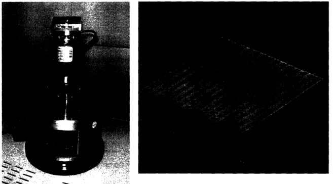
The need to visualize, create, and control objects on an atomic level has led to the development of advanced machinery capable of achieving these objectives. The scanning tunneling microscope, developed by Binnig and Rohrer in 1986 [1], is a tool that is widely used to obtain atomic-scale images of conductive surfaces. It provides a detailed, three-dimensional profile of the surface being scanned. Figure 1 is a picture of an STM with a scanned image of a sample grid. The scanned image is generated from the voltage reading of a piezo scanner stage that moves up and down as a sharp probe raster scans across the sample in order to maintain a constant distance between the sample and the probe's tip.

Figure 1: STM on left with a scanned image of a sample grid (150x150 microns) on right

New approaches, which improve the imaging quality of STMs, are being avidly pursued. An STM with a scanning mechanism capable of five-axis motion, as opposed to the traditional three-axis scanning mechanism currently used, could improve imaging quality. The addition of two degrees of motion, roll and pitch, allows the STM probe to be aligned at angles that approach more closely the more ideal scanning angles that lie perpendicular or normal to the surfaces being examined. Traditional three axis STM

1.2: Scanning Tunneling Microscopy Theory

A scanning tunneling microscope achieves atomic-scale resolution by using quantum mechanical tunneling of electrons. A sharp conductive tip is brought in close proximity to a sample's surface until the object's electron cloud overlaps the electron cloud of the scanning probe as shown in Figure 2. A bias voltage is then imposed between the probe and the sample thereby inducing a small tunneling current across the gap between the probe tip and the sample.

Probe Tip

Electron Cloud

Sample Surface

Figure 2: The electron clouds of the tip and the sample

The tunneling current typically begins to flow at a surface-to-tip distance of 15 angstroms at a bias voltage of 1 volt and is related to this gap, d, by the relationship in Equation 1.

I = Coe-

I is the tunneling current and C is a material property constant of the tip and sample. The value of 01/2 is typically 2 when the surface-to-tip distance is on the order of a few

angstroms [2]. It is important to note that the relationship of distance to current is exponential. If the surface-to-tip distance changes slightly, the tunneling current is substantially changed. The features of surfaces can be characterized with great accuracy as a consequence of this natural phenomenon.

A scanning tunneling microscope is operated most commonly in constant current mode. Using this mode the tunneling current is kept at a constant value for a fixed bias voltage. The sample is moved relative to the tip as a piezo actuator raster scans the sample under the tip. As the probe moves over discontinuities, pits, ridges, and bumps on the surface, it tracks the topography of the sample in a way that maintains a constant surface-to-tip distance while maintaining the constant current constraint imposed by the controller. The image of the surface is constructed from the feedback control voltage on the vertical z-piezo element as it corrects for changing surface-to-tip distance.

1.3: How Five-Axis Scanning Could be Achieved and the

Challenges Accompanying this Process

Creating an STM with a five-axis scanning mechanism would be an ambitious and complex task. The HexFlex, a six-axis, monolithic, compliant stage invented by Professor Martin Culpepper, could be used to achieve this goal. A diagram of the HexFlex is given in Figure 3. Its stage is moved when the tabs are actuated. This device

could be used to scan and tip-tilt the sample and probe tip of an STM relative to each other to improve the perpendicularity of the probe to surface being scanned.

Grounded Base Support Moving Stage Actuating Tab Figure 3: HexFlex

The tiexFlex is a good choice for achieving five-axis motion for a number of reasons. Its monolithic, planar design simplifies manufacturing and decreases costs and production time. Other methods of increasing the number of degrees of freedom in the scanning process would require moving parts, which could suffer frictional losses and wear. This would lessen the durability, precision and accuracy of the machine. The HexFlex consists of a single piece of metal that is capable of repeatably achieving a location and then elastically returning to its original position.

Adding two degrees of rotary freedom to the scanning system of an STM would raise issues that need to be considered. It is clear that if roll and pitch were integrated into the scanning process, the point about which the rotation would need to occur would be at the surface of the sample directly below the probe. Controlling the rotation so that it occurs only about this point, which is constantly moving across the surface during

scanning, is a difficult problem that traditional three-axis STM imaging systems do not face.

Other challenges arise when extra degrees of freedom are added to the STM imaging system. Recreating the actual image representing the sample's topography, for example, would be a very different process if roll and pitch were added. No longer would the z-voltage alone create the image displayed by the computer. Geometric relationships would need to be worked out to recreate the image of the surface based on the history of angles rotated and distances traversed along all axes during scanning.

This would not be an easy task. Furthermore, one would also need to determine when the probe should be tilted, what direction it should be tilted in, and by how much it should tilted relative to the surface to improve imaging quality. Providing solutions to these problems would complicate the STM's scanning/control system tremendously. A

few possible ways of controlling tilt are:

a) If two probes were used, the forerunner probe could first measure the surface with a standard three-axis system to gain a sense of the topography. Then, based on the information collected by the first probe, the second probe following behind could be tilted with the Hex-Flex system.

b) A single probe could be used to scan each line of the sample repeatedly, using the information gathered with each scan to tilt the probe with increasing precision until the machine's image converges to a stable or "true"

topography.

c) A special probe could be built that is capable of detecting the direction and magnitude of several contact/electrostatic-surface forces on its tip as it scans

over the sample's surface. Based on this information, the nature of the surface's topography could be determined well enough to allow the probe to know when and by how much to tilt as it approaches dips and hills.

d) Past trends in scanned data could be used to predict a sample's topography that could allow the probe to guess when and by how it should tilt.

If any of the ideas listed above were implemented into the scanning control system, it would slow the STM's scanning speed and response time substantially. The five-axis STM is, therefore, not without its disadvantages. As such, it is important to know if the benefits of a five-axis machine would justify the additional complexity and

Chapter 2: How Adding Tilt Could Improve Imaging

Quality

This chapter describes the three main sources of STM scanning errors: geometric constraint, lateral effect, and tip bending. Arguments are presented, which justify the lessening of these errors if an STM capable of five-axis scanning were developed.

2.1: Geometric Constraints

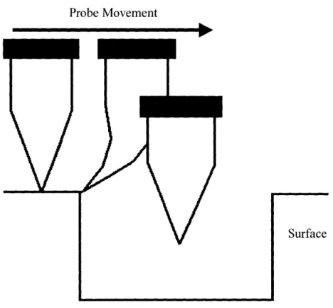
The images obtained with an STM are not necessarily an accurate depiction of the true topography of the surface. Errors may be created during scanning due to the geometry of the tip and the surface being scanned. Dips and cracks in the sample can go undetected in the image displayed simply because the probe's tip cannot fit inside the pits and cracks in the surface being scanned. The size and geometric shape of the probes used in the scanning process are, therefore, important in determining the STM's resolution capabilities.

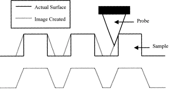
A typical STM probe can be roughly modeled as a triangle. This geometry can explain the shape of the images of some walls as the tip steps off a vertical or steep drop. The wall of the dip can appear much shallower than it really is because of the interaction of the geometric shapes involved.

By comparing the geometries depicted in Figures 4 and 5, one can see that an STM capable of only three degrees of motion along the x, y, and z-axes can generate imaging errors that may be avoided with an STM probe capable of moving with five degrees of freedom. A relatively fine-tipped probe that can tilt could trace out walls and

corners that a relatively large tip fixed in a vertical position could never accurately trace. The benefits of decreasing imaging errors by making the probe's geometry and scanning orientation more compatible with the sample's geometry may compensate for the added complexities inherent in a five-axis STM scanning system.

Probe

le

... ... .

Fige. 4: Ersaenm igiatatnlT . h f e

Figure 4: Errors made in imaging with a traditional STM with 3 degrees of freedom

ple

.. ... , ...

.. . ... . ... .. . . .. .. . . .. .. .. . . . . .. . . .... . .

Figure $: How errors in imaging could be greatly reduced if an STM probe could tilt

I s Actual Surface

... Image Created

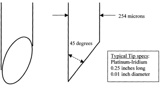
-Knowledge of the exact geometry of a probe's tip improves one's ability to interpret the images created by that probe. A closer look at the manufacturing process used to make an STM tip also offers insight into the geometry of probe tips. Digital Instruments' Platinum-Iridium tips are created by crudely cutting simple cylindrical wires with scissors at approximately a 45° _{angle. This geometry is shown in Figure 6. Images}

created by such a tip will show some asymmetry if the cut, elliptical face of the probe is facing in any direction other than the one that is farthest away from the line of travel. Also note the diameter of the probe, which determines the curvature and size of its tip radius. This tip must fit within a sample's cracks in order to properly resolve them.

254 microns

Figure 6: Probe geometry

The actual tip geometry varies from probe to probe. A closer look at a randomly selected probe tip with a Scanning Electron Microscope (SEM) reveals the existence of tiny chunks of metal jutting out from the probe's cut surface. These splinters can be seen

,pical Tip specs: Eatinum-Iridium 25 inches long )01 inch diameter

in the SEM images shown in Figure 7. It is from these sharp splinters that the current actually tunnels between the sample and probe. The difficulty in determining the true tip geometry stems partly from the multiplicity of splinters, any one of which the current could choose to tunnel through during the scanning process, the obscure shapes and orientations of these splinters, as well as the possibility that some may change shape or break off during scanning.

According to Digital Instruments, however, the typical tip radius is approximately 200-500 nm. This specification is consistent with the measured tip radius of the randomly selected probe shown in Figure 7 that has a tip radius of about 400 nm. Based on the size and shape of such a tip, one can see that in order for a probe to drop off a vertical step into a cavity, the probe would have to traverse at least a full tip radius from the cavity's edge. The bulk shape of the tip, therefore, affects the shape of the images created.

Splinters

I~~~~~~~~~~~~~~~~~~~~~~~~~~~~~~~~~~~~~~~~~~~~~~-_.313

LNW18N-Figure 7: Actual tip geometry as shown by a Scanning Electron Microscope (Note especially the scale bars for appropriate dimensional comparisons.)

2.2: Lateral-Effect Problems May Be Improved by Adding Tilt

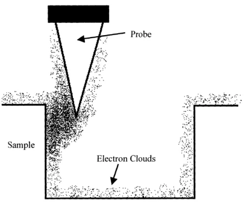
When measuring surface topography with STMs, some electrons may tunnel into the side of the probe rather than through the end of its tip. This is called the Lateral-Effect [3]. This may happen, for instance, if a wall is closer to the side of the probe than to its tip. Figure 8 is a depiction of this phenomenon occurring. When this happens, the machine "perceives" a closer tip-to-surface distance. The probe will, therefore, not correctly track the true surfaces topography near steep walls. Once the probe has moved away from the wall, the perceived tip-to-sample distance approaches the correct value and the tip will track the surface with better accuracy.

Sample

(,~--~

Electron Clouds

I;..

Figure 8: The current tunnels from the sample's lateral wall to the probe instead of from the sample's surface directly below the probe.

The error due to the lateral effect may be reduced if the probe can be tipped and tilted. Therefore, a five-axis STM with a good tilting control system could minimize imaging errors due to the lateral effect.

2.3: Tip-Bending Problems May Be Improved by Adding Tilt

Another phenomenon that causes imaging errors is referred to as the "tip-bending" problem [3]. The error is due to deflection of the tip under the influence of electrostatic forces. These forces, for instance, tend to bend the tip as it tries to step down a ledge on the sample as shown in Figure 9. The STM may not perceive a change in the tip-sample gap if the tip deflection is large enough. At some point the tip will travel far enough off the ledge so that the electrostatic forces are no longer strong enough to bend the tip. The tip will then return to its normal shape. This problem can be noted when images appear asymmetric and have a characteristic flaw on a particular side of a dip in the sample. Asymmetry in the scanned image of a symmetrical shape occurs because tip bending does not occur when the tip rises out of the dip on the object's other side.

Probe Movement

Figure 9: The probe bends toward the wall due to electrostatic forces between the sample and the tip as it steps off a ledge. No bending occurs when the tip rises out of a dip.

If a five-axis stage is used in conjunction with a probe, which has high axial stiffness, the deflection and therefore the error may be minimized.

Chapter 3: Experiment

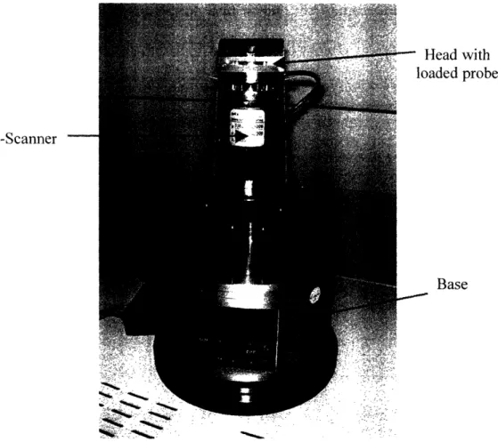
An experiment was conducted to determine the effect of changing the angle between the tip axis and the normal to the sample surface. Seven angles were tested within a range of -13° to + 1 3°. The experiment was conducted using a standard Multi-Mode Scanning Probe Microscope with a Digital lila controller from Digital Instruments. The microscope is shown in Figure 10. The scanning tunneling microscope mode was used in this experiment.

3.1: Apparatus

Platinum-Iridium probes were loaded into the STM's head as shown in Figures 10 and 11. The head was mounted on the top of the J-scanner. The head rests atop three adjuster screws, which enable the probe to be lowered carefully toward the sample. The sample was secured to the scanning platform with double-sided carbon tape. The piezo scanner stage moves the sample back and forth in the x-y plane and is capable of extending and retracting in the z-axis. The probe remains fixed to the head of the scanner during scanning.

- Head with loaded probe

Base

Figure 10: Multimode Scanning Probe Microscope in STM mode

Probe

Sample

--Figure 11: Top view of the STM's head J-Scanner

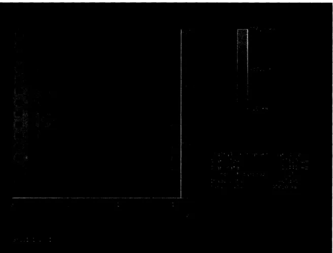
A standard grid sample from Digital Instruments was used for the experiment. The grid consisted of square cavities that were 5 x 5 microns square and 180 nanometers deep. The squares were separated from each other by 5 microns. A small section of the 1 x 1 cm sample grid was scanned using the STM. Two image displays created by the nanoscope software are shown in Figures 12 and 13.

Figure 13: 3-D display feature of the nanoscope software for visualizing the image

3.2: Method

The first challenge in conducting the experiment was to develop an adequate means to tilt the probe relative to the sample. The probe that was mounted on the head of the STM could be tilted via three adjuster screws as shown in Figure 14.

Tip

STM head Sample

Raise the screws to til the head an(

probe

Figure 14: Mechanism for tilting the probe tip with respect to the sample

A convention for the sign of the tilt angle was established and is shown in Figure 15. The operator views the tip as if he/she were standing where the photographer of the pictures in Figure 10 and 11 stood to take the pictures.

Negative Tilt Zero Tilt Positive Tilt

II _ II < I Probe I

III

Figure 15: Convention for the sign of the tilt angle

Initially, the probe was tilted to -13° and lowered to a random section of the

to the computer. Keeping the probe tilted to -13° , another random location on the

sample was selected for scanning. Again five consecutive cavities were scanned at this new location. This procedure was carried out three additional times at random locations on the sample grid. This resulted in a total of five groups of five consecutive, scanned cavities at - 13 .

The probe was then tilted to - 9°. At this angle the sample was scanned again

using the same procedure as that noted above. Five more groups of five consecutive cavities were scanned at five locations on the grid. The same process was conducted with the probe placed at probe angles of - 5° , 0, ° 5°, 9°, and 13 . A total of twenty-five

unique cavities were scanned at seven different tilt angles between positive and negative

13°0.

The data was analyzed using the software provided by Digital Instruments. The slopes of the cavity walls could be ascertained and displayed. A cross-section of a scanned sample is shown in Figure 16. The software kept track of important points by using markers, whose locations are defined by the user along the cross-section.

The markers were placed at the edge and base of the steps as shown in Figure 16. The slopes on both sides of each cavity were calculated using the horizontal and vertical position at each marker. An example of a Nanoscope display is shown in Figure 17.

Image 4r]

"--Line of interest selected by the user and its corresponding cross-sectional image is shown above

Figure 16: Determining the slopes of the cavity walls using markers in the Section Analysis tool

Figure 17: An example of a typical Nanoscope display

IJ I I LJ LJ

DEE DE

F.-I

I I I I I I

Appendix A contains tables with all measurement data. Note that all left-wall slopes are negative, and all right-wall slopes are positive.

Chapter 4: Results

4.1: Data Plots

Figures 18 and 19 are plots of the cavity wall slopes measured at different probe-tilt angles. Each triangle represents the mean value of the wall slopes of the corresponding twenty-five cavities scanned at the particular probe-tilt angle displayed by the horizontal axis of the plot above or below it. The vertical error bars represent a single

standard deviation.

Probe's Tilt Angle [degrees] -13 u --0.005 0.01 0.015 0.02 0.025 0.03 0.035 --0.04 0.045 0.05 --9 -5 0 4. -A.; 5 9 13 .4....

Figure 18: Line of best fit that relates the left wall slopes of all the cavities scanned to the angle of tilt used for scanning

0.06 E 0.05 C E .E. 0.04-a) '_ uC 0.03-.._ o 0.02-0 0. o 0.01 -u) tn +4 -13 -9 -5 0 5 9 13

Probe's Tilt Angle [degrees]

Figure 19: Line of best fit that relates the right wall slopes of all the cavities scanned to the angle of tilt used for scanning

E C E ax_w %._ '0 en U;3 o -0 a) 0. 0 C) co k ' .k

--..

Both plots reveal a linear trend between wall slope and probe-tilt angle. The wall slopes vary from -0.01 nm/nm to -0.04 nm/nm on the left walls and 0.04 nm/nm to 0.01 nm/nm on the right walls as the probe is tilted from -13 to 13 . The slopes of the lines of best fit for the plots in Figures 18 and 19 are both -0.001 change in wall slope per degree of probe-tilt. This is a significant number because it says that as the probe is tilted appropriately through an angle change of one degree, the slopes of the walls imaged will "improve" by a change in slope of about -0.001. That is to say, the imaged wall slopes will more nearly approach the infinite slopes of the cavity's vertical walls.

The percent errors in measured slopes for the left and right walls are plotted in Figures 20 and 21. In order to obtain expressions for the percent errors, the walls of the cavities were assumed to have a slope of 10 nm/nm. This slope was selected because it is three orders of magnitude larger than the typical slopes measured by the STM and, therefore, appropriate to use for estimating the slopes of the vertical walls of the cavity. There is a clear linear trend in both plots. The slopes of these lines are the values of interest because they are the change in percent error per degree tilt of the probe. The slope of the plot in Figure 20 is 0.0099 change in percent error per degree of tilt and the slope of the plot in Figure 21 is -0.0087 change in percent error per degree of tilt. The average of the absolute value of these slopes is 0.0093 change in percent error per degree of tilt. This number tells how much less error there will be in the image scanned when the probe is appropriately tilted a single degree.

Angle of Probe-Tilt [degree] -15 ' 99.65 --99.7 -99.75 -99.8 -99.85 -99.9 -99.95 -10 -5 0 5 10

Figure 20: Percent error in left wall slopes versus probe-tilt

Angle of Probe-Tilt [degrees]

-15 -10 -5 -99.55 99.6 --99.65 -99.7 -99.75 -99.8 -99.85 -99.9 0 5 10 15

Figure 21: Percent error in right wall slopes versus probe-tilt

Data taken from consecutive cavities at five different locations on the sample are shown in Figure 22. In this case, the data was scanned with a probe tilt of - 9° . The

15 L. 0 IL-L. w 0) 0 Co L_ a. I-l 0 . C C) a. n t2 . I I I . I I I I I I I I . I . I . . I I . . . .

diamonds represent the mean values of the five consecutive cavities' right wall slopes. The vertical error bars represent a single standard deviation. The wall slopes of the consecutive cavities scanned at a common location on the sample had smaller spread than the spread of the mean values of the five consecutive cavities' slopes at different locations. This finding suggests that the sample's wall slopes vary uniformly over the sample and depend somewhat on the location of the cavities on the sample.

U.UO -n Co L- 0.05-, 0.04 'a 0.03 coE_{s) r} 0.02 o 0.01-0 0 U) 0

4,

+

first second third fourth fifth

Locations on the Sample

Figure 22: Typical spread of the data collected from five consecutive squares at five different locations (This data was taken with the probe at a -9° tilt.)

4.2: Discussion and Interpretation

A number of significant trends are evident in the results obtained in the previous section. The data demonstrates that as the probe is rotated from a negative tilt to a positive tilt, the slope of the left wall of the pit will transition from a small, negative slope

to a larger, negative slope, i.e. from shallow to steep. The right wall's slope transitions from a larger, positive slope to a smaller, positive slope, i.e. from steep to shallow. Figure 23 illustrates these trends. This observation is in agreement with the trends predicted from the geometric constraints of the system.

Negative Tilt Zero Tilt Positive Tilt

Probe

% /~~~~~~~~

7

Left Slope: shallow Left Slope: moderate Left Slope: steep Right Slope: steep Right Slope: moderate Right Slope: shallow

Figure 23: Trends in wall slopes based on probe's tilt

The question as to whether STM images could be improved with the ability to tilt the probe relative to the sample in a controlled fashion while scanning is confirmed by these findings. When the probe tip is tilted at a positive angle while scanning left walls and when the probe tip is tilted at negative angles while scanning right walls, the images created are more accurate-i.e. when the tip is angled toward the wall, the imaged walls become steeper. Building a five-axis STM with at least a 130 tilting capability would, therefore, improve imaging accuracy.

By how much, then, would the image accuracy be improved? The qualitative answer to this question is presented in the section preceding this one. It was determined that as the probe is tilted through an angle change of one degree, the slope of any of the

walls imaged would improve by a change in slope of about -0.001 nm/nm. This tiny change in slope may, at first, seem trivial. Consideration must, however, be given to the fact that the range of wall slopes measured is between 0.01 nm/nm to 0.04 nm/nm for right-wall slopes and -0.01 nm/nm to -0.04 nm/nm for left-wall slopes. These slopes are only a single order of magnitude larger than the change of slope (-0.001) that results from a single degree of change in the probe's tilt angle. If a five-axis STM were, therefore, capable of tilting a probe 10° with respect to the sample, the corresponding change in

wall slope would be around -0.01 nm/nm. This change in slope would only eliminate 0.093% of the imaging error. This improvement in image quality may seem trivial, but it is not. A change in slope of-0.01 nm/nm is a significant improvement in the imaging of wall's slopes when we consider that the range of measured wall slopes are on the same order of magnitude as 0.01 nm/nm.

The shallowness in the measured slopes of the actual, vertical walls of the cavities may be explained in a number of ways. The slopes of the cavities' walls in the sample examined were supposed to be vertical and should have approached infinity. This was not the case. As previously mentioned, the imaged wall slopes ranged from 0.01 nm/nm to 0.04 nm/nm. These slopes are nearly horizontal! This finding is a sobering reminder of the enormity of imaging error that needs to be eliminated before STMs can truly and accurately image sample topography.

The reason for the shallowness of these measured slopes can best be explained by the scanning phenomena described in Chapter 2. If a typical probe with a tip radius of 400 nm were to step down a vertical-walled cavity 180nm deep, which was in fact the case in this experiment, the best slope capable of being imaged just from the principles of

geometric constraint alone would be 0.45 nm/nm. The maximum cavity slopes measured were 0.04 nm. This discrepancy is the result of the lateral effect, tip bending, and other unexplained quantum phenomena.

Chapter 5: Sources of Error

Some mistakes were made during the course of this experiment, which may explain some of the outlier slopes recorded as well as the standard deviations observed. Metallic shielding, for instance, should have been used while scanning with the STM to prevent electromagnetic interference. A sound shield was also discovered shortly after the experiment had been performed, which if used, might have reduced some of the noise caused by the vibration of air.

5.1: Errors using Probes

Two other source of error stems from the repeated use of probes and from changing probes. Probes become dull with use as their tip changes shape during scanning. Probe-tip alignment with the sample also affects imaging. Although care was taken to align the sheared, elliptical face of the probe in a direction that was facing away from the line of travel during scanning, controlling the accuracy of that alignment was not an easy task due to the tiny size of the probe tip.

5.2: Errors due to Contamination

Contamination of the sample with dust may have caused additional error. The experiment was conducted over the course of a month due to complications with the STM that was used. The sample was accidentally left exposed to the air on the stage of the scanner during this time instead of being kept in its case while not being used. During this time, contaminates could have landed in the cavities and may have resulted in errors. Before each scan, however, the sample was cleaned with isopropanol and acetone. It was later learned that samples are supposed to be cleaned with compressed gas from a dust-off can. The relatively narrow standard deviations documented in the data, however, argue against the seriousness of these problems as major sources of error.

5.3: Errors due to the Nature of Scanning

The STM's scanning control system itself could also be a source of imaging error. If contaminates were on the surface of the sample, the varying electrical properties of these materials would introduce error into the system. Analysis of equation (1) in section 1.2 shows that changes in the material constants could disrupt the scanning system of the STM and cause imaging errors.

5.4: Errors in Data Acquisition

Aligning the red markers on the edge of the cavity's ledge and base was not always a straightforward task. The location where the wall began and ended was, in

many cases, unclear and the markers were placed on the image contour at the discretion of the operator.

Despite these possible sources of error, standard deviations were not larger than 0.03 nm/nm and did not obscure the rather clear linear relationship between slope and probe tilt.

Chapter 6: Conclusion

The effect on image quality of tilting the probe tip in an STM relative to the sample's surface during scanning was explored and found to improve measurements of slope. A change in slope of -0.001 per degree of probe tilt was demonstrated. This change corresponds to 0.0093% less error in the image quality.

Although this improvement was small, it demonstrated that improvement was possible and related the angle change to slope improvement. Whether this degree of improvement is significant enough to justify development of a HexFlex-based, five-axis STM system is still open to question. The addition of two extra degrees of freedom to an STM's scanning system would substantially complicate the scanning process and the control system's mechanical design and circuitry, not to mention their effect on the expense of manufacturing. Nevertheless, the construction of such a scanner would be a step forward, however small, in helping scientists peer with greater clarity into the nanoworld.

References:

[1] M. Schmid, "The scanning Tunneling Microscope- What it is and How it Works" http://www.iap.tuwien.ac.at/www/surface/STM_Gallery/stm_schematic.html

[2] D.A. Bonnell, "Microscope Design and Operation" Chapter 2 in "Scanning Tunneling Microscopy and Spectroscopy", pp. 7-10

[3] V.M. Ichizli, M. Droba, A. Vogt, I.M. Tiginyanu, H.L. Hartnagel, "Peculiarities of the Scanning Tunneling Microscopy Probe on Porous Gallium Phosphide", in Atomic Force Microscopy/Scanning Tunneling Microscopy 3, edited by S.H. Cohen and M.L.

Lightbody, Kluwer Academic/Plenum Publishers, 1999, pp. 158-164

[4] R.A. Lewis, S.A. Gower, P. Groombridge, D.T.W. Cox, and L.G. Adorni-Braccesi, 1990, "Student Scanning Tunneling Microscope", pp. 38-41

[5] R.K. Sears, B.G. Orr, and T.M. Sanders, Jr., "A Scanning Tunneling Microscope For Undergraduate Laboratories", pp. 427-430

Appendix A

This section contains the complete data tables of all the wall slopes measured using the STM. Table 1 is the table containing the left wall slopes and Table 2 is the table containing the right wall slopes.

Table 1: Left wall slopes collected for each angle of probe tilt.

(Slopes of a common color mean they were determined from consecutivecavities.)

-13 -9 -5 0 5 9 13 -0.01620928 -0.01328736 -0.01722683 -0.0234733 -0.0347294 -0.05988019 -0.03425778 -001481958 -0,01388 -0.01671173 -0.029472 -0.01561068 -0.08542317 -0.02491608 -0.01582982 -0.01515479 -0.0169653 -0.015104 -0.018130152 -0.0627704 -0.03635613 -001738874 -0.1611107 -0.01871672 -0.02502112 -0.01877016 -0.0610107 -0.03970451 -0.01666642 -0.01533833 -0.018885666 -0.02802908 -0.01666581 -0.05119422 -0,0437022 -0.01256784 -0.00951477 -0.01385495 -0.01118942 -0.04432441 -0.03914906 -0.0440805 -0.00590482 -0.01094881 -0.009504798 -0.01096195 -0.03072985 -0.0256768 -0.04083897 -0.01035026 -0.01361595 -0.00888567 -0.01283237 -0.02983386 -0.03592859 -0.03932024 -0.01178889 -0.01151818 -0.011348688 -0.01874152 -0.02074786 -0.02690976 -0.02680075 -0.00939989 -0.0115419 -0.01364586 -0.018660614 -0.03211223 -0.02138322 -0.0671545 -0.00798464 -0.01241553 -0.01497895 -0.03318742 -0.043458 -0.04182986 -0.04018064 -0.00834089 -0.01632949 -0.01479465 -0.03068455 -0.047780452 -0.03207127 -0.02116921 -0.00821465 -0.01448549 -0.0168932 -0.01575768 -0.01291008 -0.01615182 -0.04486201 -0.00828191 -0.0147628 -0.01482821 -0.0278038 -0.040100353 -0.02729181 -0.01651968 -0.00716638 -0.01733703 -0.01564903 -0.01828515 -0.02732253 -0.02565855 -0.06032973 -0.00399819 -0.00664977 -0.01507712 -0.0155157 -0.04744387 -0.0339561 -0.02699299 -0.01018618 -0.00723549 -0.02090469 -0.02498208 -0.0225685 -0.0246011 -0.06440018 -0.00423848 -0.00635011 -0.01044914 -0.01750521 -0.048204183 -0.01937047 -0.0244461 -0.00693481 -0.0079843 -0.018551388 -0.02180087 -0.03197834 -0.01644793 -0.0236867 -0.01549012 -0.01082216 -0.02369054 -0.01942016 -0.04048384 -0.02747317 -0.0391879 -0.0122606 -0.01718289 -0.02468512 -0.03014361 -0.00732928 -0.01391951 -0.050115 -0.01297603 -0.01906485 -0.036121138 -0.03270642 -0.01530873 -0.01840664 -0.03754704 -0.01490326 -0.01038966 -0.040083967 -0.02191104 -0.02578977 -0.03819057 -0.05125186 -0.0125932 -0.00942941 -0.02885449 -0.02671946 -0.0225456 -0.03187241 -0.02433355 -0.01464426 -0.0125888 -0.0198336 -0.019159089 -0.0259580 -0.01785879 -0.02867749

Table 2: Right wall slopes collected for each angle of probe tilt

(Slopes with a common color were derived from consecutive cavities.)

-13 -9 -5 0 5 9 13 0.02973056 0,03362722 0,036128 0.06387282 0.0100454 0.020176948 0,01509719 0.06049715 0.0381888 0.0376448 0.01751424 0.01087654 0.02415264 0.01735121 0.08241815 0.03417711 0.03053883 0.06249552 0.00806738 0.01971021 001858073 0,03360768 0.03265156 0.03301888 0.01225171 0.00763008 0.02092364 001475183 0.04612076 0.03122594 0.0391217 0.013515811 0.01091921 0.01767424 001644524 0.02094464 0.02818432 0.00928764 0.01229824 0.02531334 0.02481024 0.01800847 0.02291584 0.0305164 0.0071535 0.0103244 0.01624064 0.02072064 0.021641 0.01555119 0.02808448 0.014358125 0.01272827 0.01962752 0.02468608 0.01912179 0.07983718 0.0348755 0.0162660 0.01324709 0.03794127 0.02104682 0.01963209 0.08046183 0.0267648 0.02680866 0.01436544 0.02115968 0.035846674 0.02189472 0.01408516 0.02135372 0.02008193 0.07721059 0.03009753 0.01753856 0.0095673 0.01759054 0.03018568 0.0240550 0.04527558 0.03625682 0.02920411 0.01196843 0.01678545 0.02559136 0.0340342 0.0483117 0.0152512 0.02265590 0.0129864 0.0111934 0.02584565 0.03634641 0.03070451 0.01784483 0.05622856 0.00819027 0.02790559 0.03589074 0.02529792 0.04405448 0.02104823 0.01452241 0.00988588 0.05232829 0.05518265 0.01682425 0.04213742 0.038087517 0.01359884 0.01606558 0.05066175 0.02500992 0.0143051 0.02660224 0.03514323 0.013978337 0.01265155 0.05931188 0.0357255 0.01876643 0.02764288 0.03016704 0.012833212 0.01365579 0.04638405 0.05427131 0.0088345 0.0303718 0.02473216 0.014162476 0.01256797 0.04628421 0.03931854 0.02083557 0.0286848 0.020988497 0.0287651 0.0150677 0.03540819 0.0634334 0.04314057 0.01635321 0.02012151 0.0052207 0.001851061 0.02931058 0.03275478 0.03577554 0.0125568 0.02100736 0.03406892 0.01949659 0.03204352 0.0456292 0.0424468 0.03151319 0.02159488 0.01112576 0.02180322 0.03597424 0.05883272 0.03042803 0.03105496 0.02243456 0.0137369 0.02194882 0.0342355 0.0529222 0.0736419 0.02308939 0.0325039 0.00998123 0.01819508 41

MITLibraries

DISCLAIMER OF QUALITY

Due to the

condition of

the

original material, there are unavoidable

flaws in this reproduction. We have made every effort possible to

provide you with the best copy available. If you are dissatisfied with

this product and find it unusable, please contact Document Services as

soon as possible.

Thank you.

Some pages in the original document contain