The effect of an unbiased grid in determining the kinetic energy balance of the northern hemisphere.

____g_&N MXjSpH g 9NERM &MANCX OF TfMNORTH

by

HAROLD CYRIL WALKER

B.S., Pennsylvania State University (1963)

SUBMITTED IN PARTIAL FULFILLMENT OF THE REQUIREMENT FOR THE

DEGREE OF MASTER OF SCIENCE

at the

MASSACHUSETTS INSTITUTE OF TECHNOLOGY August 18, 1969

Signature of Author

Department of Ateorology, 18 August 1969

Certified by

Thesis Supervisor

Accepted by

Chaip n, fepartmental Committee on Graduate Students

Harold Cyril Walker

Submitted to the Department 1969 in partial fulfillment degree of Master

of Meteorology on 18 August of the requirement for the of Science

ABSTRACT

For the past several years computational studies of such topics as the northern hemisphere kinetic energy balance and re-lated subjects have been performed by the Planetary Circulation Project of the Massachusetts Institute of Technology. Numerous integrals required were recently evaluated directly from a five-year period of observations using a network of nearly 800 stations. The stations, however, were concentrated primarily over temperate latitude continents, and the data from maritime and tropical areas were compartively sparse. The question then arises whether the results are representative. The problem undertaken in this thesis was to select a subset of more uniformly spaced stations and to recompute the zonal kinetic energy balance. This was accomplished and the results are presented.

Thesis Supervisor: Victor P. Starr Title: Professor of Meteorology

I INTRODUCTION

II ANALYTIC CONSIDERATIONS

III METHOD OF ANALYSIS

IV DEVELOPING AN UNBIASED GRID

V ANALYSIS VI EVALUATION Eddy Terms Coriolis Terms Other Considerations Summary of Conclusions TABLES 2 - 17 BIBL IOGRAPHY ACKNOWLEDGEMENTS

4. LIST OF FIGURES

1. Complete set of stations used in the June 1968 18 computations

2. Reduced set of stations of unbiased network used 19 in March 1969 computations

3. Vertical meridional cross sections of wind com- 23 ponents and stream function

4. Vertical meridional cross sections of momentum 25 transport and angular velocity

5. Vertical meridional cross sections of the genera- 27 tion of zonal kinetic energy

6. Vertical meridional profiles of the quantities in 29 Figs. 3-5

7. Illustration of the problems involved in computing 35

[IT]

LIST OF TABLES

1. Generation of zonal kinetic energy in the atmosphere 8 2. Station list and percentage of observations 41

3. 60-month vertically averaged wind components 63

4. 60-month vertically averaged profiles of momentum transport 64 5. 60-month vertically averaged generation of kinetic energy 65

6. Spring vertically averaged wind components 66

7. Spring vertically averaged profiles of momentum transport 67 8. Spring vertically averaged generation of kinetic energy 68

9. Summer vertically averaged wind components 69

10. Summer vertically averaged profiles of momentum transport 70 11. Summer vertically averaged generation of kinetic energy 71 12. Fall vertically averaged wind components 72 13. Fall vertically averaged profiles of momentum transport 73 14. Fall vertically averaged generation of kinetic energy 74 15. Winter vertically averaged wind components 75 16. Winter vertically averaged profiles of momentum transport 76 17. Winter vertically averaged generation of kinetic energy 77

For more than 200 years the theory of the general circula-tion of the atmosphere has been undergoing continuous modificacircula-tion as inadequate hypotheses give way to improvements based on observa-tional fact. As late as the mid-1930's efforts by Hadley (1735), Ferrel (1856,1859) and others had resulted in what appeared to be an acceptable three-cell, atmospheric general circulation scheme to account for the mid-latitude mean westerlies and low-latitude mean easterlies. The different wind regimes were thought to be caused essentially by the balance between Coriolis forces and friction acting on zonally averaged flow. However, Jeffreys (1926) suggested

that eddy actions might be able to account satisfactorily for the required poleward transport of angular momentum. A transport was required since the rotation of the earth against the mean easterlies in the tropics would impart a torque on the atmosphere, and, con-versely, westerlies would impart a torque on the earth at higher latitudes. Clearly, a poleward transport mechanism for angular momentum must exist to account for the balance.

Unsatisfactory explanations in terms of mixing length theory were unable to cope with the requirement that momentum be trar-s-ferred from~ regions of low angular velocity (tropics) to regions of higher angular velocity. Further, traditional eddy viscosity, if acting alone, would require the atmosphere to revolve eventually in solid rotation. Some combination of transport by the mean meri-dional circulation and turbulent mixing was the mechanism originally

some modified mechanism must be present.

In 1948 V. P. Starr, following Jeffreys, proposed that tilting troughs and elliptical closed circulations could account for the

required momentum transfer needed to maintain the westerlies against friction. A NE-SW tilting trough would transfer positive momentum poleward across latitude circles in the northern hemisphere. The

transport could be determined by calculating the covariances of the wind components multiplied by appropriate terms to account for the density of the air and the shape of the rotating earth. The stbject is so well known by now that no further explanations are in order here.

Subsequent momentum transport computations by Widger (1949), Mintz (1951) and Starr and White (1954a) produced convincing evidence

that the required transport was in fact accomplished mainly by the eddies (tilting troughs and ridges, etc.). Transport by the mean meridional circulation was found to be small. Later calculations using more data were designed to better evaluate the magnitude of the transport by transient eddies, standing eddies, and the mean meridional circulation. The Planetary Circulation Project at M.I.T. collected five years of daily upper air observations from May 1, 1958 to April 30, 1963 for 704 stations in the northern hemisphere, and the calculations were repeated. In these computations the zon&l kinetic energy balance was also evaluated.

The results were both encouraging and perplexing. Contributions to the kinetic energy of the mean zonal easterlies and westerlies by the eddies were significant as had been shown a few years earlier.

The Coriolis force acting on the mean meridional circulation was found to be applying a brake on the atmosphere, but to such a large extent that very little kinetic energy would be left over for dissipation by frictipn.

Efforts over the next year were devoted to an evaluation and improvement of the objective analysis techniques used, but the

most significant change resulted when the calculations were repeated in June 1968 after about 95 stations were added in the tropics, Values obtained from this larger list of 799 stations are shown in TABLE 1 opposite the row labeled June 1968. The data listed after the row labeled March 1969 will be explained later. The 1968 results were more acceptable than previous computations in that the contribution from the mean meridional circulation term was some-what less negative; however, the trouble that existed in the pre-vious analyses was still evident. Magnitudes in the seasonal com-putations were still unacceptable. In spite of the improvements with the addition of the tropical stations, the Coriolis term (mean meridional circulation term) still remained too large. The change after the addition of the tropical stations suggests that results

could be further enhanced by a better network of stations. Even with the added data from the tropics, the vast majority of sta-tions is still located over the most densily populated land areas of Europe and North America, and comparatively few stations exist over oceans, especially tropical oceans. The question arises whether the Coriolis term is sensitive to a land-ocean bias in the stations

20 -1

Expressed in units of 10 ergs sec , the numbers in the following table represent the values obtained for the generation of kinqtic energy in the northern hemisphere for the periods indicated by the prooesseo described in the left-hand column. The firat not of values represent those calculated in June 1968 from the full list of 799 stations. The second entry represents the values obtained

in March 1969 from the reduced set of 206 stations. The difference between the two calculations is the third set of numbers.

5 Years Spring Summer Fall Winter

60 months 15 months 15 months 15 months 15 months

Transient Eddies June 68 6.9739 5.5754 5.101 6.9200 4.8967 Mar 69 6.8452 5.4923 4.739 7.2024 5.6653 Difference -0.1287 -0.0831 -0.362 +0.2824 +0.7686 Standing Eddies' June 68 0.3678 0.4553 1.855 2.1121 1.2801 Mar 69 0.2515 0.4044 1.377 1.6820 -0.1683 Difference -0.1163 -0.0509 -0.478 -0.4301 -1.4484

Mean Meridional Circulation

Jun 68 -5.251 -12.4950 -6.921 3.3490 -4.439

Mar 69 ~ -3.653 -10.6103 -2.048 2.7529 -3.961 _ Difference +1.598 +1.8847 +4.873 -0.5961 +0.478

used in the computations. What would be the result if a net-work of stations were chosen so that the land-ocean bias were reduced as much as possible? This question was investigated in some detail, and the results will be discussed after some analytic considerations are presented.

II. ANALYTIC CONSIDERATIONS

The following is essentially that development presented by Starr (1968) and is included here for completeness.

A quantity may be defined as comprising an average value and

a departure from that average value. In our problem involving com-ponents of the wind field the portion of the wind that blows from the west,&L., can be defined as

--

?

(1)

where the brackets represent the longitudinal average along a lati-tude circle,

at

(2)

and 14* represents the departure. Here represents longitude. The quantity,t4( , may also be described in terms of its time mean,

where the bar represents the time mean and the prime represent3 the departure from its mean value. An analogous treatment, of course, applies to the southerly wind component, V . The latter will 'e positive toward the north, and "- will be positive toward the east.

11. we need to consider the product of that quantity and the poleward component of the wind,

V

. The transport of momentum per unit volume would then be V , where is the density. If the

expan-sions (1) and (2) are substituted for M4. and V , we have

where such quantities as U' are discarded because they are zero. Here .will be assumed sufficiently constant at a constant pressure surface along a latitude circle to be removed outside the brackets.

The first right-hand term represents the effect of the mean meridional circulation. The second term is a time and longitudinally

averaged product of temporal deviations and represents the effect due to transient eddies. The last term is the equivalent represen-tation for standing eddies. Time averaging has been performed before space averaging.

Considering now the transport of absolute angular momentum, across a latitude surface, we may write

V(5)

M

may be resolved into the part due to the rotation of the earth,

1,.

, and a part due to LA. Thus

M e- (5).

where J2.=

R

COS is the distance to the axis of rotation;

RI

is the mean radius of the earth, and is the latitude. Sub-stituting into .(5) we have

./1

/0f

vc

x/P

+~~

a vcLX

I

(7)

The first integral represents the mass transport across a latitude surface and must be zero in the long-term average. The second term represents the transport of relative angular momentum.

The torque applied by Pu4 l in (7) acting across a unit area of a vertical surface of constant latitude is - Z77^-

4/

V or -a 7714 4

s (2

. Then the net torque in the zonal direc-tion upon an annular volume of width and unit depth is

- zrr

_.

puVR'eos')

')

(8)

After eliminating boundary terms, the generation of kinetic energy in a polar cap can be written, with the help of (4), as (see Starr 1968)

Vj6OS~_(

t

)(9

(10)

or the system may be written in pressure coordinates. The Coriolis effect has been included in (11) and that integral could have been written in a form symmetric with (9) and (10). See Starr and Gaut

(1969).

It can be seen from (9) and (10) that kinetic energy can be produced only when momentum is transported against the gradient of angular velocity. The Coriolis effect in (11) will result in a loss of kinetic energy whenever and

C-j

are negatively cor-related. Equations (9) and (10) may also be described as the con-version of eddy kinetic energy to zonal kinetic energy through eddy (Reynolds) stresses.

Fourier analysis by Saltzman and Teweles (1964) shows that hemispheric wave numbers 1 through 15 all furnish kinetic energy to the mean zonal flow by this negative viscous effect. Dissipation occurs through molecular stresses and by retardation by (11).

An analogous treatment of the vertical velocity would result in another set of integrals as would inclusion of boundary considera-tions. The vertical velocity is, however, small and difficult to determine, and the transport between the hemispheresacross the equa-tor must also vanish in the long-term average. The significant integrals, then, would seem to be (9), (10) and (11).

They were evaluated for the northern hemisphere by Travelers Research Center (T.R.C.), Hartford, Connecticut, through use of finite difference techniques and objective analysis methods. Programs for automatic computation were written by T.R.C. under contract with

M.I.T. and computations were performed on the UNIVAC 1108 of the U.S. Geophysical Fluid Dynamics Laboratory at Princeton.

III. METHOD OF ANALYSIS

The five years of data originally used in these analyses consisted of daily upper-air observations from all available stations in the northern hemisphere and extended as far as 20 degrees into the southern hemisphere. The data were obtained on tape from the U.S. Weather Bureau's National Records Center as Asheville, South Carolina. Programs were developed so that observations that exceeded normal expectations in various ways were discarded, hopefully eliminating most erroneous observations. By 1968, 799 stations had been checked for usable information.

At this point the time averages of Lt and V were computed for each station at each of 20 pressure levels. From these values the covariances of temporal deviations, A'v' , were developed and these were averaged in both time and analyzed in space to produce Similarly, the standing eddy term

[*

q],

was computed. From these and other quantities cross-sections were analyzed and printed out by the computer. The cross-sections were copied in drafted form so they could be reproduced.

In the objective analysis, values were determined for each 10 degrees of latitude and longitude, except near the poles where

five-degree blocks were used. From these fields values were in-terpolated at two-degree intervals. In all, the quantities [a]

and

LEC

were determined from these latter

Available data was read in at 50-mb intervals. Since most sur-face pressures are above 1000 mb, climatological values were used at that level when actual data were missing. Further, when a value

was not available at the next higher 50-mb interval, the lower value was used as a first guess for the upper value. Also, time averages for a particular station level were not computed from the data at a given point unless at least 30 percent of the total possible number of observations at that point were available.

This 30-percent cutoff was used to preclude calculating unrepre-sentative averages.

As we shall see shortly, the transient eddy term is the most

significant contributor to the generation of zonal kinetic energy, and it is this term that cannot be evaluated from a mean map without individual instantaneous observations. In the objective analysis this would not seem to present a serious problem except in certain large areas of missing data.

This, then, is a brief account of the methods used in the June 1968 computations which will be compared with the results obtained

by this writer using an unbiased network of stations instead of the

total 799 stations. Except for using fewer stations no changes were made in the method of analysis so that the effect of a land-ocean bias could be studied properly.

IV. DEVELOPING AN UNBIASED GRID

It was felt that by selecting a set of stations which were uniformly spaced and equally distributed between land and ocean areas any land-ocean bias could be reduced. It was realized at the onset that a perfectly unbiased grid could not be developed because of the available station distribution, but if the integral

(11) because less negative, we would feel that a land-ocean bias

in the original network did exist and that it had been partially corrected.

In order to develop an unbiased network it was first neces-sary to reduce the number of stations over continents (there was of course no way to add stations over the oceans). It then became essential to select only the best stations from which data were available.

The latter requirement involved checking the total number of observations recorded by each station at each of 10 pressure levels. "Good" stationsbecame those that had at least 30 percent of all available observations at all pressure levels from 850 mb to 100 mb, inclusive. "Mediocre" stations were those that had at least 10 percent at any pressure level. These latter stations were scanned for whatever usable information they contained when it became necessary to use them for lack of other data. Stations with less than 10 percent were discarded.

The vast majority of missing observations occurred at 1000 mb, 70 mb and 50 mb. But discounting these levels, 396 stations

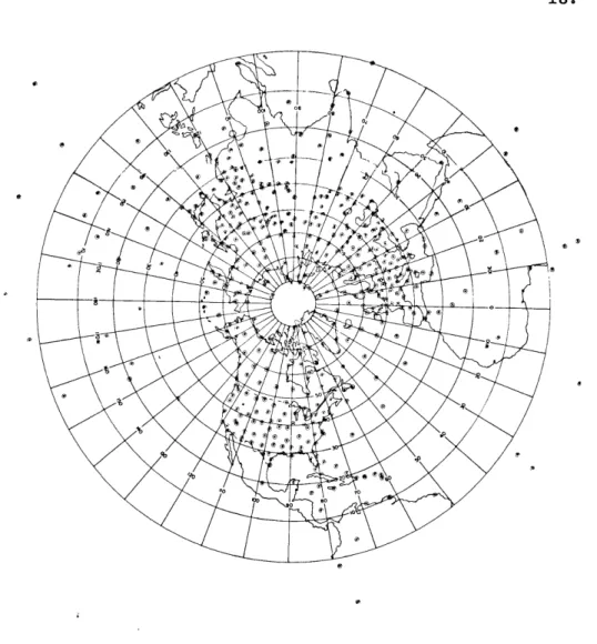
Fig. 1. Dots represent locations of stations at 400 mb which had at least 30 percent of the total

pos-sible observations available. They approximate the distribution of stations used for all levels in the June 1968 computations. The outer

lati-- tude circle represents the equator. The

addi-tional stations in the southern hemisphere were used to improve the tropical analysis.

/~~~~ @

Fig. 2. This subset of 206 stations represents a network which has a minimum land-ocean bias. Those sta-tions which have at least 30 percent data from 850 mb - 100 mb, inclusive, are represented by circles. Some stations with less than 30 percent of the data at all levels were added to improve the tropical analyses. These stations are

remained that had 30 percent at each level from 850 mb to 100 mb, inclusive. This set became the basis from which the unbiased grid was attempted.

Because some crowding still existed, 182 of these stations were eliminated. Tropical areas were deficient and 62 of the 10-percent stations were added to balance out the lower latitudes. Roughly half of the original 799 were deficient in some serious way.

The final network is shown in Fig. 2, which should be compared with Fig. 1. Th.e latter figure represents the distribution of sta-tions at 400 mb which had 30 percent of the total possible observa-tions available. The 400-mb set is reasonably representative of all levels except 1000 mb, 70 mb and 50 mb. The 30-percent cutoff used per level in the June 1968 calculations would have resulted in a map similar to this.

Looking at Fig. 2 one notices that some bias still exists and that there are virtually no data available in the eastern Pacific and very little south of 30 degrees north latitude in the Atlantic. Not apparent is the fact that practically no data were available from below 850 mb or from above 100 mb from the U.S.S.R. (This de-ficiency is currently being corrected, but the data from these levels are not included in the present computations.)

During the calculations a 10-percent cutoff was applied at

each station at each level as the data were used. A 30-percent cutoff could not be applied without eliminating absolutely essential, if mediocre, data from the tropics. The cutoff had virtually no effect

on northern latitude stations since most of those densities far greater than 30 percent.

The remaining sections of this paper will be cussion and comparison of the results obtained by the so-called unbiased grid with the computations using the complete station list.

TABLE 2 contains all of the information from biased grid was developed.

stations had

devoted to a dis-this writer using made in June 1968

un-V. ANALYSIS

The numbers presented in TABLE 1 represent the integrated values of expressions (9), (10) and (11) in ergs sec

1

for the generation of zonal kinetic energy in the atmosphere. In the 60-month column the biggest change between the June 1968 and the March 1969 computations occurred in the mean meridional circulation term.

It became less negative, as was hoped. A small change was also noted in the standing eddy term. The most stable term was the

generation by transient eddies. Roughly half of the zonal kinetic energy generated or transformed from transient and standing eddies

is dissipated by the Coriolis effect on the mean meridional circu-lation acting as a brake on the atmosphere. Of the 7.1..ergs seca1 generated, 3.7 are dissipated by this effect, leaving 3.4 units for dissipation by friction. The percentages involved here agree with the required results obtained by Gilman (1965), who derived meri-dional circulations of the southern hemisphere from indirect methods.

Seasonal values in TABLE 1 were also calculated, and the largest difference is again seen in the mean meridional circulation term. The spring values for the mean term are still much too large negative, and it would appear that the atmosphere would cease to function (see Starr, 1953) if these values represented the true

conditions in the atmosphere. Summer values seem much more realistic. In the June 1968 computations for this season, practically no energy was left over for dissipation by friction, while in the March 1969 computations, the Coriolis effect dissipated only about one-third

IU M

B

-5-10- 5 0 5 5 25 200 2

J

6 ~ -2-- -25 -5000 -- 0 -200- --600-25 - -25 -So-10 O 2 2 0~' 2000 ' - - -s C o -~~\ - - ,S ~-* 0 26 -25 S 5 -25 600- 0 2-25 -o25 -2 I3O - -z. _{C -- o} -1000 - -- --- 0 -5 0 '-O, - SC --- 4

~

0 --

~o

25 ' 25 - , 5 0 . \_1 200 - -00 0 20 400 80 0 0 40 60 80 -00 0I 0 \'25 I 1 60 0 I~5

~

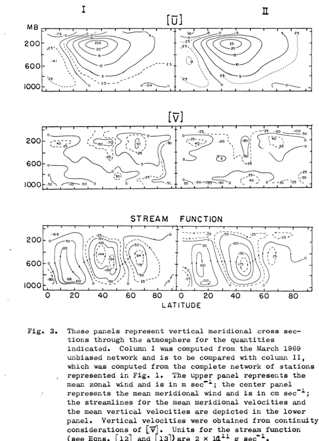
25--~ 5C/ 26 '- -SO-'40 0 -- M - 0 10 0 201\ 0 0 0 8 0 4 0 8 LAT TUDE

Fig. 3. These panels represent vertical meridional cross sec-tions through the atmosphere for the quantities

indicated. Column I was computed from the March 1969 unbiased network and is to be compared with column II, which was computed from the complete network of stations represented in Fig. 1. The upper panel represents the mean zonal wind and is in m sec

a;

the center panel represents the mean meridional wind and is in cm sec ; the streamlines for the mean meridional velocities and the mean vertical velocities are depicted in the lower panel. Vertical velocities were obtained from continuity considerations of

[3v].

Units for the stream function (see Eqns.

[12]

and

(13])

are 2 x 1 g sec .

of the total amount generated. The same type of problem seen in spring occurred in fall, except it appears that too much kinetic energy is generated. Here the Coriolis term contributed to the

total zonal kinetic energy instead of depleting it. The winter season was the only period where the standing eddy term showed a marked change in contrast to the Coriolis term which changed very little. In all computations the transient eddy term changed least of all. Because of non-linear effects the sum of the seasonal terms

i s not equal to the values computed for the 60-month period. A possible explanation for the behavior of the terms seen here will be presented after the comparison between the two sets of computa-tions has been completed.

In the vertical meridional cross sections through the atmos-phere which follow, column I represents the results obtained from the unbiased network of 206 stations. These values are to be com-pared with the results obtained in June 1968 from the complete net-work of 799 stations presented in column 2. Cross sections and profiles are presented for the 60-month period only.

The top panel in Fig. 3 represents the mean zonal wind,

[U3

in m sec~1. Plus values represent winds from the west. Both cross sections are virtually identical. The center panel represents the mean meridional wind,

[O

, positive toward the north. Here some differences are noted. The negative area in the middle latitudes has been reduced, and the positive area further north has been

MB 200 600 1000 200 600 1000 200 600 1000

[U'

Vl

Cos

2

S6

[U

V*]

COs

#

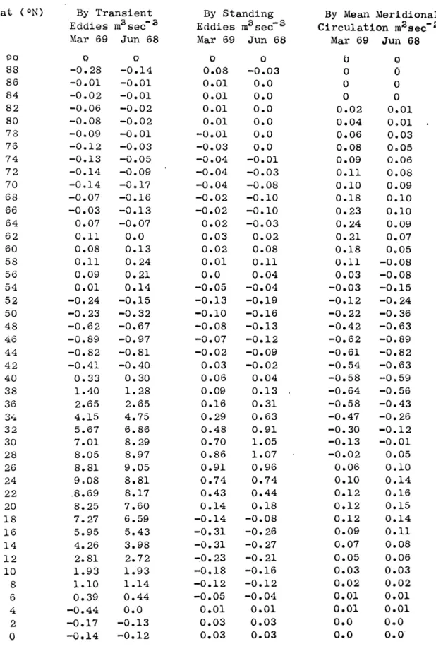
0 20 40 60 80 0 20 40 60 80 LATITUDE

Fig., 4. These vertical meridional cross sections through the atmosphere represent the northward transport of angular momentum by transient eddies (top panel) and by the standing eddies (center). The mean angular velocity of the air motions about the polar axis are shown in bottom panel. Units of the momentum transport are m2sec 2 and are to be multiplied by 2TWR. Units of angular velocity are m sec~l to be divided by the earth's radius, R, to obtain the relative angular velocity. Column I was computed from the reduced set of stations and is to be compared with column II, which was computed from the complete network of stations.

---

06--19I

-to lack of data north of 800 and are inconsequential because of the comparatively small volume of the polar cap north of 800.

The stream function at the bottom of Fig. 3 shows some signi-ficant similarities and differences. The driven cell in middle latitudes is smaller in both size and magnitude. The tropical cell is slightly larger in size, but only slightly different in magnitude. The direct polar cell is larger. The vertical motions implied in the cross sections were derived from continuity considerations of the mean meridional wind component. The picture was obtained by

fitting a stream function to the distribution of

VO

in center panel.

The analytic form of the stream function is defined by

2. 77) dS

066

+j7

Iy(12)

and

77"-2 do95~~ (13)

where CA> is < .Units are 2 x 1011 g sec

-The top two panels in Fig. 4 represent the northward transport of angular momentum evaluated across each two degrees of latitude. The values given are of

L4

7C

05$5;

showing the transport

due to transient eddies. The values in the center panel are of

Vf

COSIO

showing the effect of standing eddies. Both 2 -2

are to be multiplied by 2

7~

, the units being m sec * The transient eddy term shown in the top panel is significantly larger

MB

M[TV,]

cos2#0

Z

-([I]/Cos$

M B , , 600 1 - 0.

600-2d9 00 (Z2 %. 03 a3 1000 - * -0. - 0.2 0 . - . 200 C 0.-O-' 0 _ 0 -9-0.2 -I3 0 A %-N)1.0 -. 5 600 2 . 0.

[U] [i

cos

son

-5-05

__L _. I I I .A I I .

IU1CS$

I]cs

sin

2 00. --5 - 0 600 '6.j -00 1 ,,

~

0 100025, 00 0

~

09 -. . 0 0 - -. 0 -- 600-0 20 40 60 80 0 20 40 60 80

LATITUDE

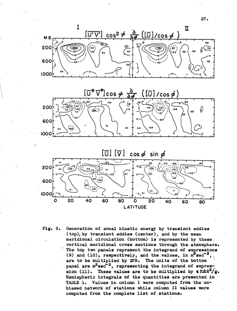
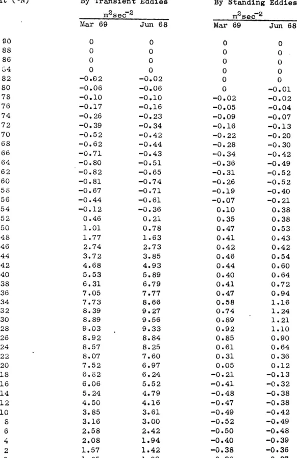
Fig. 5. Generation of zonal kinetic energy by transient eddies (top), by transient eddies (center), and by the mean meridional circulation (bottom) is represented by thesei

vertical meridional cross sections through the atmosphere. The top two panels represent the integrand of expressions

(9) and (10), respectively, and the .values, in m sec 8 ,

are to be multiplied by 2TR. The units of the bottom panel are m2sec"2 , representing the integrand of

expres-sion (11). These values are to be multiplied by 47rAR

/g.

Hemispheric integrals of the quantities are presented in TABLE 1. Values in column I were computed from the un-biased network of stations while column II values were computed from the complete list of stations.

than the standing eddy terms shown in the center panel. The main change in the computations of momentum transports by the transient eddies is the high latitude smoothing in the 1969 analysis. The

strong

counter-gradient flux of momentum at lower latitudes from regions of low angular velocity into the mean jet stream through negative viscous effects is essentially unchanged.

The mean angular velocity of the air motions about the polar axis is shown in the bottom panel of Fig. 4. This panel was obtained

from the top panel of Fig. 3. The values given are of

U6lI1

in

m sec

1,

and are to be divided by the mean radius of the earth, ..

to obtain the relative angular velocity. Because the term becomes indeterminant near the pole, very high values in this region develop in the computations and were arbitrarily eliminated from the cross sections. Except for some such residual difference in the analyses, very little change is noticed between the two computations.

Fig. 5. represents the production of zonal kinetic energy due to conversions by transient eddies (top panel), standing eddies (center panel), and the mean meridional circulation (bottom panel). The top two panels represent the distribution of the integrands of expres-sions (9) and (10) and are to be multiplied by 2 7

71c

. The units

3 -3

are m sec . The bottom panel represents the distribution of the integrand of (11) and is to be multiplied by

£

7TR./. . No significant difference exists between the two computations in the top two panels. The decrease in the values of the integral (11) represented by the bottom panel is not immediately apparent. The

29. M/S 12 6 0 -6

M3/SEC

3

K.E.

GEN

12 6 0 .- 6 -12

ERATION

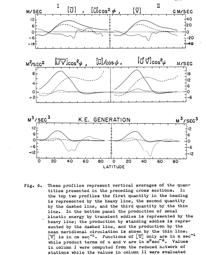
0 20 40 60 80 0 LATITUDE

Fig. 6. These profiles represent vertical averages of the quan-tities presented in the preceding cross sections. In the top two profiles the first quantity in the heading is represented by the heavy line, the second quantity by the dashed line, and the third quantity by the thin line. In the bottom panel the production of zonal

kinetic energy by transient eddies is represented by the heavy line; the production by standing eddies is repre-sented by the dashed line, and the production by the mean meridional circulation is shown by the thin line. [v] is in cm sec~1. Functions of

[I

only are in m sec~ while product terms of u and v are in m2sec 2 . Values in column I were computed from the reduced network of stations while the values in column II were evaluated from the complete network of stations.

EC 40 20 0 -20 M3/ _SEC3 12 6 0 -6 -12 20 40 60 80 - -- -- --

-positive area near 600 is larger, and even though the maximum value of the middle latitude negative region is greater, the location has

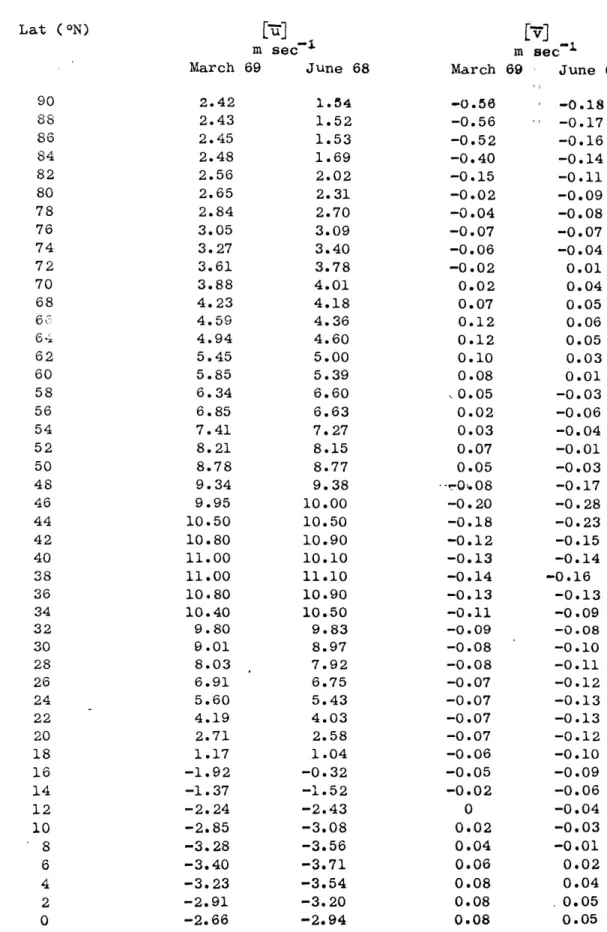
shifted sufficiently so that the vertical average is less. Fig. 6 represents the vertical averages of the quantities just described in the cross sections. Here [a3 , shown by the heavy line in the top panel, is essentially the same in both analyses, except for some smoothing at higher latitudes. The same observation holds for

£7 's

-5 $ representing the angular momentum per unit mass of the atmosphere. Units for both these quantities are m sec . The quantity of most interest in this discussion

[

-1 is shown by the thin line in the top panel and is plotted in cm sec . Since there is no net mass transport of dry air across latitude cir-cles in the atmosphere, this term should be essentially zero in the long-term average. South of about 400 the magnitude of the term was decreased by the unbiased network. North of 400 some "noise" was introduced and the term is more positive. The extreme value between

300 and 400, however, has been reduced by about one third. In the

energy calculations the vertical averages of [P] weresubtracted from values at each level before the computations were made. The resulting vertical average would then be zero as would be expected physically.

The center panel of Fig. 6 shows the vertically averaged momentum transport across any particular latitude circle and the angular velocity of the air motions about the polar axis. Momentum transport per unit mass by the transient eddies is represented by

_V

COS4

9

and is shown by the dark line. The standing eddy

transport is represented by

L7z

1

CosaJ6

and is shown by the

thin line. The angular velocity is shown by the dashed line, Units

-l 2 -2

of the latter are in m sec while the other terms are in m 2ee .

The differences between columns I and II are slight. Both columns, however, vividly illustrate the transport of angular momentum against the gradient of angular velocity.

The bottom panel of Fig. 6 is the vertically averaged distri-bution of the integrands of expressions (9), (10) and (11). The heavy line represents the generation of zonal kinetic energy by

transient eddies; the dashed lines represent generation by standing eddies, and the thin line represents generation by the mean meridional circulation. The values of the integrand of expression (11) have been converted to the same scale as expressions (9) and (10). The

reduction of I near 480N seen in Fig. 3 shows up here as a smaller negative value in the Coriolis term. The positive area to the north is also larger.

The first conclusion from examining the cross sections and profiles is that the reduction of stations produced very little

effect on the mean zonal wind or eddy terms. Significant differences are noted, however, in [V and in terms computed from it.

Throughout the discussion reference to the Coriolis term, the mean term, or the mean meridional circulation terms all refer to expression (11).

VI. EVALUATION

Two main questions now need to be considered: How reliable are the results obtained from these and previous evaluations, and why has the Coriolis term been so negative?

Eddy Terms

It has been suggested by Lorenz (1967) and by Priestly and Troup (1964) that computations of momentum transport by transient eddies are seriously affected by missing data. Every station used in the analysis had some missing observations, especially at higher pres-sure levels where strong winds exist, and presumably computations would be biased toward lighter winds. Some of this bias may have been reduced by the objective analysis which used values at lower levels as a first guess for missing data at higher levels. When the weather balloon was lost near the surface a light wind bias would be propagated upward, and when the balloon reached jet levels before being blown away, excessively high wind values would be propagated into the region of lower winds above the jets. Use of the unbiased network cannot really answer this question of light winds since the stations removed to form the network may have been biased in exactly the same way as the stations which remained, but the fact that the results computed from the reduced network of stations were virtually unchanged is encouraging.

The question concerning the adequacy of the existing network of stations in the northern hemisphere can be answered somewhat more emphatically. Ideally, one would want observations every few degrees

but of course, this is impossible, and since no important changes were noted when only one-fourth of the available stations were used suggests that the same results would be obtained if more stations

were somehow added and that the atmosphere had been sampled

adequately,

at least for processes involving transient and standing eddies. Further,.it was felt that since expressions (9) and (10) for the eddy generation of zonal kinetic energy involve a triple product of the wind speed components, reducing the total number of stations

would eliminate some extreme values and would result in a smoothing that produced smaller values of the expressions. Some smoothing did occur, as seen in the profiles of Fig. 6, but the overall values of the integrals was not reduced significantly, in contrast to the value of the Coriolis term, which did change.

Coriolis Term

One possible explanation for the behavior of the Coriolis term is that

[IV

represents a small difference between large quantities and is therefore too sensitive to handle. If this were entirely true, then different computations of V and terms computed from it should oscillate about some mean value and no pattern in the results should exist. Some oscillation in

(

and in the Coriolis term did result from the reduced network of stations, but the pat-tern one would expect from an atmosphere with a tropical Hadley cell, indirect Ferrel cell, and direct polar cell existed in both compu-tations. Profiles of

NO

in Fig. 6 should be zero since they represent the long-term vertical and longitudinal mean condition

and since there can be little or no net mass transport of dry air across a latitude circle. The consistency of the non-zero value and the fact that they became less negative by use of the unbiased network suggests the need for a physical, rather than a purely numerical, explanation. It was for this reason that the following

exercise was performed. The experiment was not designed to dupli-cate the objective analysis, but the same data were used.

In the experiment the value of was computed as more and more stations were added along a latitude circle. The area chosen

to study was the latitude belt extending from 50 to 60*N because of the comparatively high density of stations there. The latitude belt was then divided into 10-degree blocks from which stations were

selected. Cumulative averages were developed and the values obtained every time four more stations had been included were plotted on Fig. 7. Stations were added symmetrically so that if a station was available every time a 10-degree block was sampled a completely unbiased net-work would exist. The abscissa in Fig. 7 represents the total number of stations sampled. The small triangles along the abscissa repre-sent each cycle around the globe in an attempt to select a station every 10 degrees of longitude. The first triangle is plotted at 34, indicating that two 10-degree blocks had no stations. The ratio of the number of stations found to the number missing formed what was called the bias, which is also plotted. The second triangle was plotted at 61, indicating that a total of 11 stations were missing after two cycles around the globe. A 10-degree block with only one

SIAS - 4 (U s 4a ₎ . . -( -0 0.6 4 (2) SA [0] [ IS 00.6 3 -0.4 AS, 0.11 0 o _{0 0} 0 o o0 0 o00 o to 0 o t 0o

OF STATIONS SAMPLEO NUM9t1 Of STATIONS SAMPLEO

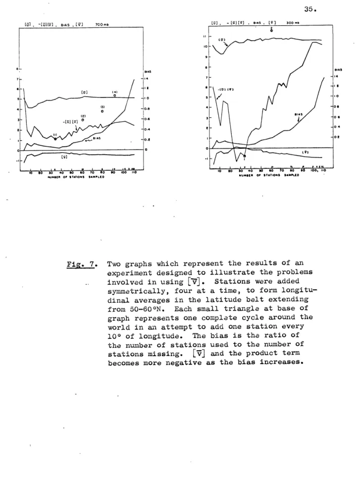
Fig. 7. Two graphs which represent the results of an experiment designed to illustrate the problems .. involved in using

[v.

Stations were added

symmetrically, four at a time, to form longitu-dinal averages in the latitude belt extending from 50-600N. Each small triangle at base of graph represents one complete cycle around the world in an attempt to add one station every 100 of longitude. The bias is the ratio of the number of stations used to the number of stations missing.

[v)

and the product term becomes more negative as the bias increases.

station would produce a missing station on every cycle after the first one.

Results obtained at 700 mb are plotted in the left-hand por-tion of Fig. 7 next to the values obtained for 300 mb. BothE§3 and are plotted in m sec

1

against the left-hand scale. Their product is also plotted on the same scale although the units of

the latter are taken negative. Negative values of the product were plotted to facilitAte comparison on the same graph.

In both graphs values of [2 and lK1 appear to vary by

about the same magnitude, but the percentage of variation for

[0

is much larger because of its- smallness. At 700 mb, for example,

doubles from 0.25 m sec

1

to slightly greater than 0.50 m sec It is interesting to note that the most positive values of _'3

occur when the bias is also the smallest. At this point one could assume that almost all geographical bias, or asymmetry in station location, had been eliminated. In each instance up to six cycles

the absolute value of

[O

increased each time the biased increased.

The product term, -j9[vI , also varied in the same way. At 300 mb the effect was more pronounced, and

Es]

and the product term even changed sign at the point of minimum bias.

The profiles represent cumulative averages so that the addition of fewer and fewer stations per cycle produced a decreasing effect.

The dependence of on the symmetry is amplified further by the values obtained on each pass before they were averaged with

on pass 2 only, for example, are much larger. These values are plotted next to the circle representing the pass number.

The implication of this simple exercise seems to be that stations should be chosen symmetrically around the globe if nV is to be measured accurately. The decreasing values of N here

represent the strong bias toward Europe where the station density was the highest. One could surmise, then, that at these pressure levels winds tend to blow more from the north at this latitude in Europe than they do in the Pacific where fewer stations were located. Of course, an accurate representation of a quasi-sinosoidal weather

pattern can only be obtained if measurements are taken from both sides of the troughs and ridges.

As mentioned earlier, this exercise was not intended to dupli-cate the objective analysis used in evaluating expressions (9), (10) and (11), but merely to illustrate the problems involved in handling In the objective analysis adjacent stations and values from lower pressure levels were used to estimate values when data were

sparse. The objective analysis could not, however, create data in large areas where none was available. Hand analysis in these areas of missing data, notably the eastern Pacific and Atlantic oceans, produced no better results than the objective analysis; see Starr

(1969). If either of these regions had persistent south winds,

then would be too large negative since the positive values

in the region of missing data could not be included in the longi-tudinal average.

This bias was precisely the problem under investigation in this thesis. Data from the oceans could not be increased but the bias from the-continents was decreased and MV became larger algebraically.

The large seasonal variations of

[Vj

may also be attributed, at least in part, to the same effect. In the Pacific, for example, if mean southerly winds existed in the region east of about 1550, then and the Coriolis term would be too large negative. If, on the other hand, seasonal shifts in weather patterns produced persistent north winds in this region of no stations, then

[Sj

and terms computed from it would be much too large positive. This type of reasoning is not restricted to the Pacific; it applies to any portion of the earth where the network of stations is too sparse .for the objective analysis to handle adequately. It seems from charts

of average cloudiness taken from satellite pictures that a special physical condition of some magnitude exists in the eastern Pacific. See, for example, Sadler (1968). Further, data being gathered by the University of Wisconsin suggests that the region is occupied by clouds of all types (low, middle and high) which seems to indicate some sort of dynamics other than air-sea interaction. Synoptic experience (Sanders, 1969) suggests that numerous cirrus streaks are present, indicating a possible southwest-to-northeast jet stream or wind flow. Further investigation of this area, possibly from an investigation of airline Doppler wind reports, is in order.

the Coriolis term, is that the negative values are due to a

biased sampling of the sinosoidal wind patterns of the atmosphere. This suggestion is emphasized by the fact that the unbiased

net-work produced more reasonable values for the Coriolis term for the 60-month average than were obtained using all available data in the northern hemisphere.

Other Considerations

WhilLe it is felt that asymmetry in any available network of stations is the main reason for the inaccurate values obtained

for

[OJ,

other considerations must be discussed. In the

develop-ment of equations (9), (10) and (11) boundary integrals were omitted as were vertical motion terms. Either or both of these may produce a significant effect. Reliable vertical motions are difficult to obtain, and it may be some time before such effects as diabatic heating, for example, can be included in the formulations of

ver-tical motions. Inclusion of boundary integrals is more feasible, and they will be evaluated in the near future by the Planetary Circulation Project. See Starr and Gaut (1969).

The fact that

LEI

was not zero in the vertical averages seen

in Fig. 7 may also be due to errors in upper wind measurements-and it may not be possible to produce values of which are much better. Ideally, one should calculate confidence limits for and the Coriolis term in order to determine if the changes seen by using the unbiased network are significant. Unfortunately, such

limits of present computer facilities.

Momentum transport calculations for the tropics by Kidson (1968) varied between odd and even years, possibly due to the

well-known biennial oscillation. 'Data in this study comprised a five-year average and one might suspect that a bias is indicated. Further, work by Newell et al (1969) suggests a biennial variation in the strength of

the Hadley circulation. But the five-year sample used suggests a some-what equal sampling of the different effects noticed on odd and even years.

Summary of Conclusions

In spite of the questions still unanswered, it would seem that this study has shown that processes involving transient and standing eddies have been evaluated as well as they could be evaluated even with a greater number of stations in sparse data areas of the northern hemisphere. This conclusion is supported by the fact that no important changes were noted in the values obtained when the existing network of stations was reduced by three-fourths.

In order to measure the mean zonal wind a symmetric network of stations is probably needed. The large seasonal variation in the Coriolis term may be due to seasonal shifts in weather patterns which move in and out of regions of the earth where observations are not

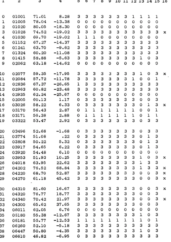
-EXPLANATION OF TABLE 2: The following table represents a summary of stations used in the computations.

The columns are identified as follows: 1. Sequence (dictionary) number 2. W.M.O. block and station number 3. Latitude 4. Longitude 5. 1000-mb level 6. 850-mb level 7. 700-mb level 8 500-mb level 9. 400-mb level 10. 300-mb level 11. 200-mb level 12. 100-mb level 13. 70-mb level 14. 50-mb level 15. Overall rating

16. "x" means used in subset

During the five-year period a total of 1800 observations (once daily) were possible. If a station recorded at least 540 observa-tions (30 percent) the figure "3" appears in columns 5-14, which

represent various standard pressure levels. If a station did not rate a grade of "3", but had at least 180 observations (10 percent), the figure "1" appears in the appropriate column. Levels with less

than 10 percent were given a figure "O".

A similar procedure was used in column 15 to summarize the

results of the preceding columns. If the station had 30 percent at each level from

850

to 100 mb, inclusive, it receivod an overall rating of "3". If it had no usable data (i.e., less than 10 percent),

it received an overall rating of "0" in column 15. An "x" in column 16 means the station was used in the unbiased grid developed by

this writer.

The rating system is summarized below: (d

=

percentage of observations).

Ratings for Columns 5-14 3 d

>

30% 1 10%

<

d

<

30% 0 d

<

10%

Overall Rating, Column 15

3 d > 30% for all levels, 850-100 mb, inclusive 1 10% < d

<

30% at any level

0 d

<

10% at all levels

In all there was a total of 799 stations, of which 689 had usable data;

396 had 30 percent for each level from 850 to 100 mb, inclusive; 206 stations were used in subset, of which

TABLE 2: Station List and Percentage of Observations 1 2 4 5 6 7 8 9 101112131415 16 01001 01005 01020 01028 01030 01152 01241 01324 01415 02062 02077 02084 02836 02963 02935 02005 03026 03170 03171 03322 03496 03774 03808 03917 03920 03953 04018 04202 04220 04270 04310 04320 04340 04300 06011 05180 06181 06260 06447 06610 3 3 0 0 0 0 3 3 0 0 O 3 3 3 3 3 3 3 3 0 0 3 71.01 78.04 80.05 74.52 69.70 67.27 63.70 60.20 58.88 63.18 59.35 57.72 67.37 60.82 62.24 60.13 58.22 56.43 56.38 53.47 52.68 51.08 50.22 54.65 54.48 51.93 63.95 76.52 68.70 61.18 81.60 76.77 70.42 65.62 62.05 55.38 55.77 52.10 50.80 46.82 8.28 -13.38 -18.30 -19.02 -19.02 -14.37 -9.62 -11.08 -5.63 -14.62 -17.95 -11.78 -26.65 -23.48 -25.67 1.17 6.33 2.87 2.88 2.92 -1.68 .22 5.32 6.22 6.10 10.25 22.62 68.84 52.87 45.42 16.67 18.77 21.97 37.65 6.76 -12.67 -12.53 -5.18 -4.35 -6.95

1 2 3 4 5 6 7 8 9 10 11 12 13 14 15 16 40 07110 48.45 4.42 3 3 3 3 3 3 3 3 1 1 3 41 07145 48.77 -2.02 1 3 3 3 3 3 3 3 1 1 3 42 07170 48.07 -5.03 0 1 1 1 1 1 1 1 0 i 1 43 07180 48.70 -6.22 0 1 1 1 1 1 1 1 0 0 1 44 07354 46.85 -1.72 1 3 3 3 3 3 3 3 1 3 3 45 07510 44.85 .70 3 3 3 3 3 3 3 3 1 1 3 x 46 07645 43.87 -4.40 3 3 3 3 3 3 3 3 1 1 3 47 08001 43.38 8.37 1 1 1 1 1 1 1 0 0 0 1 48 08159 41.68 1.07 0 3 3 3 3 3 3 3 3 3 3 49 08221 40.47 3.57 0 3 3 3 3 3 1 0 0 0 1 50 08302 39.62 -2.70 1 3 3 1 1 1 1 0 0 0 1 51 08495 36.15 5.35 1 3 3 3 3 3 3 3 1 1 3 x 52 08509 38.75 27.09 3 3 3 3 3 3 3 3 1 3 3 x 53 08521 32.63 16.90 0 0 0 0 0 0 0 0 0 0 0 54 08536 38.77 9.15 3 3 3 3 0 3 3 3 0 0 1 55 08594 16.73 22.95 0 0 0 0 0 0 0 0 0 0 0 56 10035 54.53 -9.55 3 3 3 3 3 3 3 3 1 3 3 57 10184 54.10 -13.38 1 3 3 3 3 1 1 0 0 0 1 58 10202 53.37 -7.22 3 3 3 3 3 3 3 3 0 3 3 x 59 10338 52.47 -9.70 3 3 '3 3 3 3 3 3 0 3 3 60 10393 52.22 -14.12 1 3 3 3 3 3 3 1 0 0 1 61 10454 51.85 -10.77 0 1 0 0 0 0 0 0 0 0 J. 62 10486 51.12 -13.68 0 3 3 3 3 3 1 1 0 0 1 63 10513 50.87 -7.13 1 1 1 1 1 1 1 1 0 1 1 64 10610 49.95 -6.57 0 1 1 1 1 1 1 1 0 1 1 65 10739 48.83 -9.20 0 3 3 3 3 3 3 3 1 3 3 66 10866 48.13 -11.70 0 3 3 3 3 3 3 3 0 3 3 67 11035 48.25 -16.37 0 3 3 3 3 3 3 3 0 3 3 68 11518 50.10 -14.28 0 3 3 3 3 3 3 1 0 0 3 69 11934 49.07 -20.25 0 3 3 3 3 3 3 3 0 0 3 70 12330 52.42 -16.85 1 3 3 3 3 3 0 0 0 0 1 71 12374 52.42 -26.97 3 3 3 3 3 3 3 1 0 0 1 72 12425 51.13 -16.98 3 3 3 3 3 3 1 1 0 0 1 73 12577 50.28 -21.43 0 0 0 0 0 0 0 0 0 0 0 74 12843 47.43 -19.18 3 3 3 3 3 3 3 3 1 0 3 75 13130 45.82 -16.03 3 3 3 3 3 3 3 3 1 1 3 x 76 13276 44.78 -20.53 0 3 3 3 3 3 3 3 1 1 3 77 13334 43.52 -16.43 3 3 3 3 3 3 3 3 1 1 3 78 15120 46.77 -23.60 0 3 3 3 3 3 3 3 0 1 3 79 15420 44.50 -26.08 1 3 3 3 3 3 3 3 0 1 3

4 5 6 7 8 9 10 11 12 13 14 15 16 1 2 80 81 82 83 84 85 86 87 88 89 90 91 92 93 94 95 96 97' 98 99 100 101 102 103 104 105 106 107 108 109 110 111 112 113 114 115 116 117 118 119 15614 16044 16080 16239 16242 16320 16420 16560 16596 16622 16716 17030 17062 17130 17220 17280 17606 20046 20047 20069 21007 20274 20292 20353 20667 20674 20744 20891 21358 21432 21504 21647 21824 21946 21965 21982 22113 22165 22217 22522 3 42.82 46.03 45.47 41.80 41.80 40.65 38.20 39.25 35.83 40.52 37.90 41.28 40.97 39.95 38.40 37.92 35.15 80.62 80.45 79.50 78.07 77.50 77.72 76.95 73.33 73.50 72.38 -23.38 -13.18 -9.28 -12.60 -12.23 -17.95 -15.55 -9.05 -14.45 -22.97 -23.73 -36.33 -29.80 -32.88 -27.17 -40.20 -33.28 -58.05 -52.80 -76.98 -14.22 -82.23 -104.28 -68.58 -70.04 -80.23 -52.73 71.98 -102.47 76.15 -152.84 76.00 -137.90 -112.83 -143.23 -128.92 -147.88 -162.40 178.53 -33.05 -43.30 -32.43 -34.78 74.65 73.18 71.58 70.62 70.63 70.97 68.97 68.65 67.13 64.98

1 2 3 4 5 6 7 8 9 10 11 12 13 14 15 64.58 61.72 61.80 69.77 69.40 68.47 67.65 67.47 66.53 65.12 65.78 64.92 61.67 61.63 60.68 60.97 60.43 68.50 67.55 66.77 120 121 3 22 123 124 125 126 127 128 129 130 131 132 133 134 135 136 137 138 139 140 141 142 143 144 145 146 147 148 149 150 151 152 153 154 155 156 157 158 159 -40.50 -30.72 -34.27 -61.68 -86.17 -73.60 -53.02 -86.57 -66.53 -57.10 -87.95 -77.82 -50.85 -90.23 -60.43 -69.07 -77.87 -112.43 -133.38 -123.40 22550 22802 22P20 23022 23074 23146 23205 23274 23330 23418 23472 23552 23804 23884 23921 23933 23955 24125 24266 24343 24507 24621 24688 24759 24790 24793 24817 24908 24944 24959 25042 25123 25173 25399 25428 25551 25563 25594 25677 25703 64.17 -100.07 0 63.77 -121.62 0 63.27- -143.15 0 62.02 -129.72 0 61.80 -148.80 0 62.70 -149.10 0 61.27 -108.02 0 60.33 -102.27 0 60.40 -120.42 0 62.08 -129.75 0 69.75 -167.67 0 68.80 -161.28 0 68.92 -179.48 0 66.17 -169.83 0 65.08 -160.62 0 64.68 -170.42 0 64.78 -177.57 1 64.43 -173.23 3 63.03 -175.42 0 62.93 -152.43 0