HAL Id: hal-00297079
https://hal.archives-ouvertes.fr/hal-00297079
Submitted on 9 Apr 2008
HAL is a multi-disciplinary open access
archive for the deposit and dissemination of
sci-entific research documents, whether they are
pub-lished or not. The documents may come from
teaching and research institutions in France or
abroad, or from public or private research centers.
L’archive ouverte pluridisciplinaire HAL, est
destinée au dépôt et à la diffusion de documents
scientifiques de niveau recherche, publiés ou non,
émanant des établissements d’enseignement et de
recherche français ou étrangers, des laboratoires
publics ou privés.
A multiscale approach for precipitation verification
applied to the FORALPS case studies
A. Lanciani, S. Mariani, M. Casaioli, C. Accadia, N. Tartaglione
To cite this version:
A. Lanciani, S. Mariani, M. Casaioli, C. Accadia, N. Tartaglione. A multiscale approach for
pre-cipitation verification applied to the FORALPS case studies. Advances in Geosciences, European
Geosciences Union, 2008, 16, pp.3-9. �hal-00297079�
www.adv-geosci.net/16/3/2008/
© Author(s) 2008. This work is distributed under the Creative Commons Attribution 3.0 License.
Geosciences
A multiscale approach for precipitation verification applied to the
FORALPS case studies
A. Lanciani1,2, S. Mariani2,3, M. Casaioli2, C. Accadia4, and N. Tartaglione5
1Inter-Universities National Consortium for Physics of Atmospheres and Hydrospheres (CINFAI), Camerino, Italy 2Agency for Environmental Protection and Technical Services (APAT), Rome, Italy
3Mathematics Department, University of Ferrara, Ferrara, Italy 4EUMETSAT, Darmstadt, Germany
5Physics Department, University of Camerino, Camerino, Italy
Received: 25 August 2007 – Revised: 14 December 2007 – Accepted: 23 January 2008 – Published: 9 April 2008
Abstract. Multiscale methods, such as the power spectrum,
are suitable diagnostic tools for studying the second order statistics of a gridded field. For instance, in the case of Nu-merical Weather Prediction models, a drop in the power spec-trum for a given scale indicates the inability of the model to reproduce the variance of the phenomenon below the corre-spondent spatial scale. Hence, these statistics provide an in-sight into the real resolution of a gridded field and must be ac-curately known for interpolation and downscaling purposes. In this work, belonging to the EU INTERREG IIIB Alpine Space FORALPS project, the power spectra of the precipita-tion fields for two intense rain events, which occurred over the north-eastern alpine region, have been studied in detail. A drop in the power spectrum at the shortest scales (about 30 km) has been found, as well as a strong matching between the precipitation spectrum and the spectrum of the orography. Furthermore, it has also been shown how the spectra help un-derstand the behavior of the skill scores traditionally used in Quantitative Precipitation Forecast verification, as these are sensitive to the amount of small scale detail present in the fields.
1 Introduction
Mesoscale meteorology, dealing with phenomena ranging from rain bands to thunderstorms, is deeply concerned with small scale detail. Nowadays Numerical Weather Predic-tion (NWP) models are capable of producing such detail. However, their verification is nontrivial. For instance, tra-ditional skill scores (which measure point-to-point match-ing) are sensitive to small displacement errors, resulting in a double penalty effect, so that increasing forecast detail
Correspondence to: A. Lanciani
may decrease the score. This kind of first order verification can be deceptive. Higher order moments must be studied to make sure that the fields being compared are defined on grids with the same real resolution, and even if they are, that they have the same amount of small scale detail (see, e.g., Beck and Ahrens, 2004; Ch`eruy et al., 2004; Grasso, 2000; Harris et al., 2001; Tartaglione et al., 2002).
In this work, performed within the EU INTERREG IIIB Alpine Space FORALPS project (http://www.foralps.net), we have studied in detail the power spectra of the precipi-tation fields for two intense rain events which occurred over the north-eastern alpine arc. The first event took place on 16–20 November 2001, whilst the second one occurred on 8–10 September 2005. Namely, we have studied the spec-tra of three operational Limited Area Models’ (LAMs) fore-casts, and attempted to compare these results with those from a Quantitative Precipitation Forecast (QPF) intercomparison study by means of traditional skill scores (Mariani and Ca-saioli, 2008). We have also investigated how these spectra are affected by different interpolation techniques that are usually employed in QPF verification.
The rest of the paper is arranged as follows: in the next section we will define the methodology, then we will describe the observations and models data set. Afterward we will dis-cuss some results we have obtained, and finally we will draw some conclusions.
2 Methodology
2.1 Power Spectrum
The power spectrum (Wilks, 1995) can be an effective diag-nostic tool to study the higher order moments of a gridded field and its scale dependency (Goody et al., 1998). The 2-D spectrum E(kx, ky) of a real field φ (x, y), where kxand ky
4 A. Lanciani et al.: A multiscale approach for precipitation verification
Fig. 1. LAMs’ domains: ALADIN (red), QBOLAM (green), and
WRF (blue). The gray shaded area is the verification area.
are the wavenumber components, is formally defined as the Fourier transform of the autocorrelation function:
E(kx, ky)= 1 √ 2π Z dlxdlye−i(kxlx+kyly)K(lx, ly), (1) where K(lx, ly)= Z dxdyφ (x+ lx, y+ ly)φ (x, y), (2) is the autocorrelation function and lxand lyare respectively the lag in the x direction and in the y direction.
However, it can also be computed according to the Wiener-Khinchin theorem by multiplying the 2-D Fourier transform by its complex conjugate:
E(kx, ky)= 1 2π Z
dxdye−i(xkx+yky)φ (x, y)
2 . (3)
We have chosen the latter method, as it suppresses some computational noise. Moreover, a Hanning window was pre-viously used to filter the data and to reduce aliasing (Press et al., 1992).
The relationship between the model domain grid size 1 and the wavenumber grid size ˜1 is given by ˜1= (N1)−1, where N is the number of the model grid points. The largest wavenumber from which we can extract meaningful infor-mation is given by the Nyquist frequency (21)−1. Since the models are defined on different grids with different grid steps, the wavenumber ranges will be different, too. The 2-D spectrum can be presented as an isotropic power spec-trum E(k), if it is averaged angularly and k is defined as
k=qk2
x+ k2y. The width of the bands where the average is made is chosen in order to smooth the isotropic spectrum without losing any significant information.
Scaling of the power spectrum occurs when it can be writ-ten as E(k)∼k−β. In other words, the spectrum shows scale invariance if it is linear in k on a log-log plot. The absolute value of the spectral slope, that is, β, is an indicator of the fields smoothness. The higher β, the smoother, more orga-nized, is the structure.
2.2 QPF Verification
In this study, for QPF verification, we have used the equi-table threat score (ETS; Schaefer, 1990). This score is tallied up on 2×2 contingency tables (Wilks, 1995), which summa-rize in a categorical way possible combinations of forecast and observed events above or below a given precipitation threshold. For each selected threshold, four categories are then defined: hits; false alarms; misses and correct non-rain
forecasts (a, b, c and d respectively). To reduce the
sensitiv-ity of skill scores to small changes into the population of the contingency table elements, they have been calculated on a sum of daily contingency tables depending on the time period considered. Thus, for the November 2002 event scores have been calculated on five contingency tables, whereas for the September 2005 event they have been calculated over three tables.
The ETS is an accuracy measure for events, that is, it mea-sures how well the forecast “yes” events correspond to the observed “yes” events. ETS allows also for the number of hits that would be obtained purely by chance (random fore-cast). It is defined by:
ETS= a− ar
a+ b + c − ar
, (4)
where ar=(a+b)(a+c)/(a+b+c+d) is the number of model hits expected from a random forecast.
A score equal to one represents a perfect score; whilst a value close to zero or negative means that the model has a questionable forecasting ability.
3 Models data set and observations
3.1 Models
Forecasts were modelled by three LAMs (whose domains are shown in Fig. 1) the 11-km Aire Limit´ee Adaptation dynamique D´eveloppement InterNational (ALADIN; http: //www.cnrm.meteo.fr/aladin/), operational at the Environ-mental Agency of the Republic of Slovenia (EARS); the 0.1◦ QUADRICS BOlogna LAM (QBOLAM) operational at the Agency for Environmental Protection and Technical Services (APAT; Speranza et al., 2007); the hydrostatic ver-sion of the 10-km Weather Research and Forecasting (WRF; http://wrf-model.org/) model running in a research configu-ration at the Regional Meteorological Observatory of Friuli-Venezia Giulia (OSMER). Moreover, the 0.5◦ T511 L60 ECMWF global model (http://www.ecmwf.int/) is also used in the comparison.
The models differ in parameterization and discretization schemes (ALADIN and ECMWF are spectral models, while QBOLAM and WRF are finite difference models) and in both initial and boundary conditions. Global analyses and fore-casts from ECMWF are employed as initial and boundary conditions, respectively, by QBOLAM and WRF, whereas
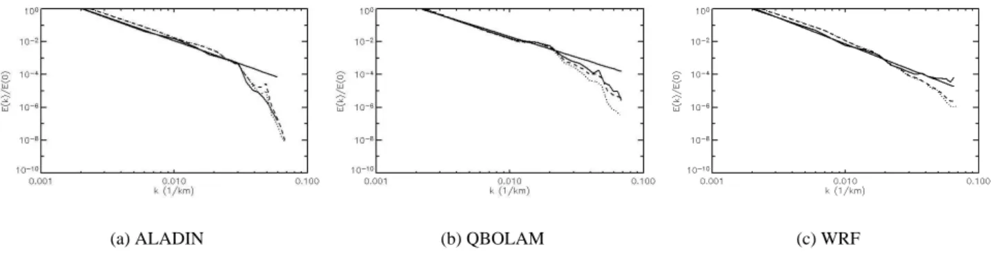
(a) ALADIN (b) QBOLAM (c) WRF
Fig. 2. Power spectrum of the 16 November 2002 24 h accumulated precipitation forecast: original grid (solid line), bilinear interpolation
(dotted line) and remapping (dashed line). A linear fit on the first part of the original spectrum is also shown.
(a) ALADIN (b) QBOLAM (c) WRF
Fig. 3. Same as Fig. 2, but for the 9 September 2005 forecast.
ALADIN employs ARPEGE (Action de Recherche Petite Echelle Grande Echelle; http://www-pcmdi.llnl.gov/) anal-yses and forecasts. Moreover, 24 h ALADIN runs, starting at 00:00 UTC, are used, while the other two LAMs are initial-ized at 12:00 UTC of the previous day for a 36 h run, and the first 12h of each run are discarded as a spin-up.
The models considered differ also in horizontal grid size. Since the intercomparison results may be sensitive to such difference, precipitation forecasts have been also post-processed on two common verification grids (with grid size of 0.1◦and 0.5◦respectively) by means of bilinear interpola-tion and also remapping1(e.g., see Accadia et al., 2003), and accumulated at 24 h, starting from 00:00 UTC.
All these differences notwithstanding, all the models (in-cluding the hydrostatic WRF) consider precipitation a diag-nostic variable. As such, it is calculated after all the prognos-tic variables have been advected. This is parprognos-ticularly impor-tant for ALADIN, because as a spectral model its dynamics take place in spectral space, whereas the microphysics take place in physical space.
1Remapping is performed by subdividing each verification grid
box into n×n sub-boxes (in this case, n=13). Then the value of
the nearest native grid point is assigned to each sub-grid point. The average of these sub-grid point values produces the remapped value of the verification grid point.
3.2 Observations
For the November 2002 event, precipitation data have been obtained from 766 working rain gauges belonging to the networks of APAT [former Italian National Hydrographic and Marigraphic Service (SIMN) network], Agenzia Re-gionale per la Protezione dell’Ambiente (ARPA) of Emilia-Romagna, ARPA of Liguria, OSMER, EARS and Zen-tralAnstalt f¨ur Meteorologie und Geodynamik (ZAMG).
For the September 2005 event, precipitations have been collected from 781 working rain gauges of APAT, ARPA of Emilia-Romagna, ARPA of Liguria, ARPA of Lombardia, OSMER, EARS, and ZAMG.
In order to produce an adequate 24-h observed rainfall gridded analysis over the two common verification grids, a two-pass Barnes objective analysis scheme has been used (Barnes, 1964, 1973). This is a Gaussian weighted-averaging technique that assigns a weight to each rain gauge observa-tion as a funcobserva-tion of the distance between the gauge and the grid box center.
More precisely, call x the position of the analysis point and xk, k=1, . . . , K, the positions of the gauges within its region of influence. A first pass is performed to produce a
6 A. Lanciani et al.: A multiscale approach for precipitation verification
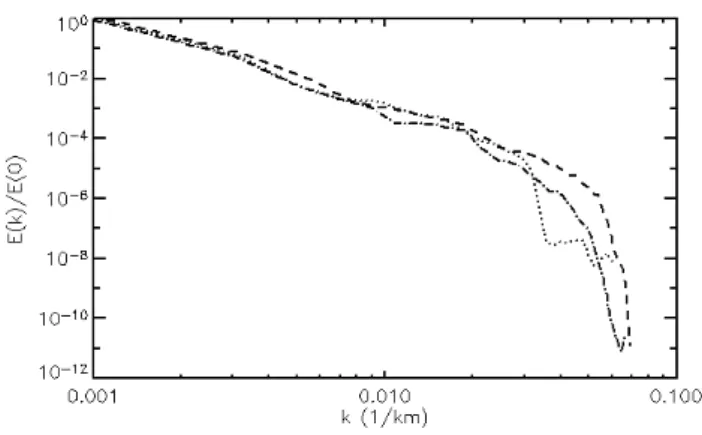
Fig. 4. Spectra of the models’ orography: ALADIN (dotted line),
QBOLAM (dashed line) and WRF (dot-dashed line).
first-guess precipitation analysis (Daley, 1991):
fA(0)(x)=
K
X
k=1
wkfO(xk), (5)
where fO(xk) is the precipitation measured at the k-th gauge and the weights are defined as
wk= exp −|xk− x|
2
4aR2
!
. (6)
In the previous equation|xk−x| is the distance between the analysis point and the position of the gauge, R is the av-erage data spacing and a is a proportionality coefficient that results in the optimal response function.
This is followed by a second pass that is needed to increase the amount of detail in the first guess:
fA(1)(x)= fA(0)(x)+ K X k=1 wk h fO(xk)− fA(0)(xk) i . (7)
The algorithm’s convergence is very fast: Koch et al. (1983) have shown that only these two passes through the data are needed to achieve the convergence of the analysis to the observations, provided that a numerical convergence pa-rameter γ ∈ (0, 1) is used to redefine R in Eq. (6) as R′=γ R in the second pass. We have used γ=0.3 and R=0.15◦.
4 Results
The spectra were calculated, using the IDL2software and its Fast Fourier Transform (FFT) and Hanning algorithms, over the intersection of all the models’ domains, i.e.: between 8.7◦W and 18.4◦W in longitude and 42.9◦N and 48.9◦N in latitude (see the shaded area in Fig. 1).
2Interactive Data Language, version 6.4, © ITT Visual
Informa-tion SoluInforma-tions, Boulder, CO, http://www.ittvis.com/.
The spectrum of the fields on their native grids displays scale invariance down to about 30 km, after which there is a fall off (we show two examples in Figs. 2 and 3). Hence, 30 km can be taken as the minimal resolution of the grids insofar as the precipitation is concerned. Actually, taking into account numerical implementation issues, such as su-perdiffusion operators that ensure computational stability, it is probably even lower (for a more throughout discussion on effective model resolution, see Frehlich and Sharman, 2007, and the references therein).
Both interpolation methods result in smoother fields, al-though bilinear interpolation slightly more so. This is more striking in the case of QBOLAM (see Figs. 2b and 3b).
The correlation between the precipitation spectra on the models’ native grid and the spectra of the models’ orography is very high, always higher than 0.98. But it is perhaps more interesting to note that the spectrum of ALADIN’s orography drops sharply for scales smaller than 3 grid steps (Fig. 4). Orography is spectrally represented in ALADIN, which is why its power spectrum should be equal to zero below about 30 km. The residual power arises from back transformation and interpolation to the physical grid.
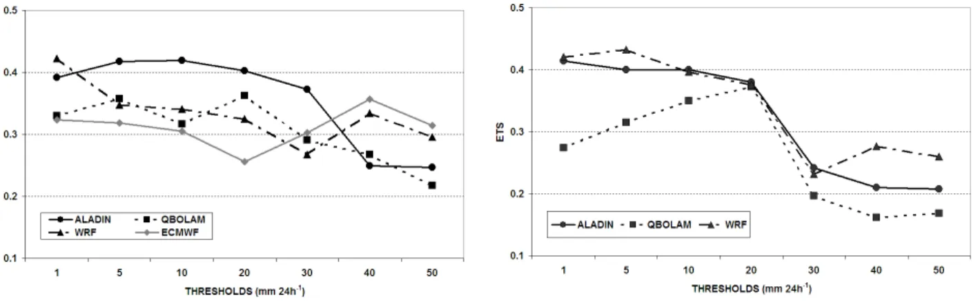
It is interesting at this point to consider also the ETS score (Fig. 5). Here we will only discuss the 2002 case. The great-est difference is on 18 November 2002 (see also Fig. 6 for an eyeball comparison between the forecast fields and the obser-vation field). As can be seen from Fig. 5a, ALADIN appears to have a better ETS than the other two models, at least up to a 30 mm 24 h−1threshold. However, its performance seems to worsen if we look at the 0.1◦grid (Fig. 5b).
As we anticipated in the introduction, this can be partly explained by the different spectral behavior of the models. Indeed, the values of β for both events can be obtained from a linear fit on the first (scaling) part of the spectra. At least for the 2002 event, ALADIN’s forecast on the original domain always has more structure than WRF’s, which in turn has more structure than QBOLAM’s. This would seem to be in contradiction with our earlier discussion on the orography spectrum. The contradiction could be explained by several reasons, both physical (absence of prognostic microphysical fields implies that none of the orographic rain lands in the lee of the mountains, amplifying small scale features; Dr. Mark
ˇ
Zagar, 2007, personal comunication) and numerical (spectral truncation entails a Gibbs effect, see Lindberg and Broccoli, 1996). However, this aspect needs further study to be fully understood.
Moreover, if we look at the spectra of the fields remapped on the same 0.1◦ and 0.5◦common grids, where the skills scores were calculated (see Figs. 7 and 8), we find that the differences among the models’ spectra are greater on the for-mer grid than on the latter.
Accordingly, ALADIN’s ETS is more penalized on the 0.1◦grid and the intercomparison should not be performed there but rather on the 0.5◦ grid. On the other hand, from Fig. 5a we see that the models’ scores are much more
(a) 0.5◦verification grid (b) 0.1◦verification grid
Fig. 5. The ETS score for the 2002 event reported as a function of the selected thresholds.
Fig. 6. Contours (in mm 24 h−1) of precipitation observed (a) and forecast by ALADIN (b), QBOLAM (c) and WRF (d) on 18 Novem-ber 2002. Forecasts are remapped on the 0.1◦common verification grid. For the observations, the contours of the 0.1◦Barnes analysis is masked over the sea.
8 A. Lanciani et al.: A multiscale approach for precipitation verification
Fig. 7. Spectra of the 18 November 2002 24 h accumulated
precip-itation interpolated on a 0.1◦common grid: ALADIN (dotted line), QBOLAM (dashed line) and WRF (dot-dashed line).
homogeneous, although ALADIN seems to behave slightly better. In a similar way, the coarser field is more penalized as the threshold increases, and this is again reflected in the ETS behavior – and, one more time, the difference is more macroscopic on the 0.1◦grid than on the 0.5◦grid, which is again coherent with our results on the spectra.
That increasing the threshold entails a reduction in the ETS of the more detailed field can be understood in the following way: If the field is not smooth, two neighboring points can have very different values. In particular, the over-lap between two slightly shifted peaks, one belonging to the forecast field and the other to the observed field, will be lesser than for a smoother forecast field. Since whatever is below the threshold gets cut, for a sufficiently high threshold what remains in the former case are two isolated peaks, entailing a double penalty error to the ETS. On the contrary, if the fore-cast is smooth there will still be an overlap resulting in both a false alarm (the forecast peak) but also a hit (where the two fields overlap).
5 Conclusions
In this work, we have studied the power spectra of the pre-cipitation fields forecast by three NWP LAMs, namely: AL-ADIN operational at EARS, QBOLAM operational at APAT and WRF operational at OSMER. For comparison and com-prehensiveness we have also considered the ECMWF fore-casts and the observations available for the two events: 16– 20 November 2001, and 8–10 September 2005. We focused on the regions of the Alpine Space as they are the subject of the FORALPS project within which this study was per-formed. Our results were threefold.
First, we found that there is a drop of the power spectrum at the shortest scales that can be theoretically resolved by these models, confirming that their real resolution is
actu-Fig. 8. Spectra of the 18 November 2002 24 h accumulated
precip-itation interpolated on a 0.5◦common grid: ALADIN (dotted line), QBOLAM (dashed line), WRF (dot-dash line) and ECMWF (solid line).
ally coarser than the grid mesh-size. Moreover, interpolation techniques further worsen the resolution by oversmoothing the precipitation fields. Between the two techniques we con-sidered, that is, remapping and bilinear interpolation, the lat-ter fares the worst. This first result is consistent with previous studies on the subject.
Second, we showed that there is a strong matching be-tween the precipitation spectra and the spectra of the orog-raphy used in the models. Although this should not come as a surprise, as the two events we studied have a clear oro-graphic component, it is important to recognize this aspect explicitly. Indeed, in this study precipitation is a diagnos-tic variable, deriving from complex processes in NWP mod-els which involve specific humidity and temperature. The two latter variables are prognostic variables and as such their equations include, for reasons owning to numerical stability, diffusion operators that cause a spectral drop. Instead, a clear and direct action of diffusion operators on precipitation has still to be fully understood.
Finally, we have related the spectra of the fields with the ETS, one of the traditional QPF verification skill scores that are often used in model intercomparison. As we expected, the lesser smoothness of ALADIN’s field was penalized by the ETS on the higher resolution (in fact, unrealistically high resolution – see above) grid. This suggests that for QPF veri-fication purposes the comparison should be performed on the coarser grid only. Otherwise particular attention must be paid in the discussion of the results, namely with regard to which model performs better. Even so, a comparison at a finer res-olution can provide physical insight into the model behavior, such as ALADIN’s tendency to produce small scale features. ALADIN’s ETS was further penalized when the thresholds in the contingency table calculation became very high.
It should be noted that, as in any other work restricted to case studies, what we have analyzed here are merely
snapshots. The subject of precipitation second order statistics deserves further study. For example, other multiscale meth-ods (e.g., wavelet decomposition) could be used. Perhaps more importantly one could try to understand the physical and mathematical reasons behind our results. Further studies along this direction, that include the use of the observations’ spectrum, are on the way.
Acknowledgements. This work was developed and funded under
the framework of the EU INTERREG IIIB Alpine Space FORALPS project (contract n. I/III/3.1/21). We thank the FORALPS partners ARPA of Lombardia, EARS, OSMER and ZAMG for providing us the observed and forecast data used in this study. Our thanks also go to the ARPA of Emilia-Romagna and of Liguria for precipitation data over their territory. Finally, we wish to thank B. Lastoria (APAT) for the help on data processing, the two anonymous reviewers for their suggestions and, last but not least, A. Speranza (University of Camerino) and G. Monacelli (APAT) for the support. Edited by: S. C. Michaelides
Reviewed by: two anonymous referees
References
Accadia, C., Mariani, S., Casaioli, M., Lavagnini, A., and Speranza, A.: Sensitivity of Precipitation Forecast Skill Scores to Bilinear Interpolation and a Simple Nearest-Neighbor Average Method on High-Resolution Verification Grids, Weather Forecast., 18, 918–932, 2003.
Barnes, S. L.: A technique for maximizing details in numerical weather map analysis, J. Appl. Meteorol., 3, 396–409, 1964. Barnes, S. L.: Mesoscale objective analysis using weighted
time-series observations, p. 60, tech. memo. ERL NSSL-62, 1973. Beck, A. and Ahrens, B.: Multiresolution evaluation of
pre-cipitation forecasts over the European Alps, Meteorologische Zeitschrift, 13, 55–62, 2004.
Ch`eruy, F., Speranza, A., Sutera, A., and Tartaglione, N.: Surface winds in the Euro-Mediterranean area: the real resolution of nu-merical grids, Ann. Geophys., 22, 4043–4048, 2004,
http://www.ann-geophys.net/22/4043/2004/.
Daley, R.: Atmospheric data analysis, Cambridge University Press, 1991.
Frehlich, R. and Sharman, R.: The use of structure functions and spectra from numerical model output to determine effective model resolution, Mon. Wea. Rev., in press, 2007.
Goody, R., Anderson, J., and North, G.: Testing Climate Models: An Approach, Bull. Am. Meteor. Soc., 9, 2541–2549, 1998. Grasso, L. D.: The differentiation between grid spacing and
res-olution and their application to numerical modeling, Bull. Am. Meteorol. Soc., 81, 579–580, 2000.
Harris, D., Foufoula-Georgiou, E., Droegemeier, K. K., and Levit, J. J.: Multiscale statistical properties of a high-resolution precip-itation forecast, J. Hydrometeor., 2, 406–418, 2001.
Koch, S. E., desJardins, M., and Kocin, P. J.: An interactive Barnes objective map analysis scheme for use with satellite and conven-tional data, J. Climate Appl. Meteor., 22, 1487–1503, 1983. Lindberg, C. and Broccoli, A. J.: Representation of topography in
spectral climate models and its effect on simulated precipitation, J. Clim., 9, 2641–2659, 1996.
Mariani, S. and Casaioli, M.: Forecast verifivication: A summary of common approaches and examples of application, FORALPS Technical Report 5, Univerit`a degli Studi di Trento, Dipartimento di Ingegneria Civile e Ambientale, Trento, Italy, 60 pp., 2008. Press, W. H., Flannery, B. P., Teukolsky, S. A., and Vetterling, W. T.:
Numerical Recipes in FORTRAN: The Art of Scientific Comput-ing, Cambridge University Press, 1992.
Schaefer, J. T.: The critical success index as an indicator of warning skill, Weather Forecast., 5, 570–575, 1990.
Speranza, A., Accadia, C., Mariani, S., Casaioli, M., Tartaglione, N., Monacelli, G., Ruti, P. M., and Lavagnini, A.: SIMM: An integrated forecasting system for the Mediterranean Area, Mete-orol. Appl., 14, 337–350, 2007.
Tartaglione, N., Lanciani, A., and Speranza, A.: Analysis of the ef-fects of numerical diffusion on some meteorological fields fore-casted by NWP models in the Mediterranean area, in: Proceed-ings of the 4th European Geophysical Soc. Plinius Conference on “Mediterranean Storm”, Mallorca, Spain, 3–5 October 2002, 4 pp., 2002.
Wilks, D. S.: Statistical methods in the atmospheric sciences: an introduction, Academic Press, San Diego (USA), 1995.