HAL Id: hal-00700643
https://hal.inria.fr/hal-00700643
Submitted on 7 Jun 2012HAL is a multi-disciplinary open access
archive for the deposit and dissemination of sci-entific research documents, whether they are pub-lished or not. The documents may come from
L’archive ouverte pluridisciplinaire HAL, est destinée au dépôt et à la diffusion de documents scientifiques de niveau recherche, publiés ou non, émanant des établissements d’enseignement et de
Influence of space and time dimensions in multi-agent
models of the free-riding collective phenomenon
Tomas Navarrete Gutierrez, Julien Siebert, Laurent Ciarletta, Vincent
Chevrier
To cite this version:
Tomas Navarrete Gutierrez, Julien Siebert, Laurent Ciarletta, Vincent Chevrier. Influence of space and time dimensions in multi-agent models of the free-riding collective phenomenon. [Technical Report] 2012, pp.22. �hal-00700643�
Influence of space and time dimensions
in multi-agent models of the free-riding
collective phenomenon
Tomas NAVARRETE GUTIERREZ
a band Julien SIEBERT
and Laurent CIARLETTA
and Vincent CHEVRIER
LORIA LORIA - Campus Scientifique
BP 239 - 54506 Vandœuvre les Nancy cedex
France
Influence of space and time dimensions in
multi-agent models of the free-riding collective
phenomenon
Tomas NAVARRETE GUTIERREZ Julien SIEBERT Laurent CIARLETTA Vincent CHEVRIER
Abstract
This report discusses how considering spatial and temporal dimensions at the modelling stage may have an influence on the outcome of the study in collective phenomena. We compared different models built on the same initial individual behaviour hypothesis of one collective phenomenon known as “free-riding” (that can be observed in peer-to-peer file sharing networks). Those models are conceived to answer questions related to the convergence and stabilization of the sharing behaviour of the users in those networks, where the non-cooperative behaviour of a subset of users may lead to the collapse of the entire network. Building up from this same individual be-haviour, we study one global analytical model and four multi-agent models, the latter ones adding space and time dimensions, which are rarely seen in the literature discussing aggregated models of the collective phenomenon in question. After discussing the a priori and the experimental conditions under which the models are equivalent, we show that the same individual decision algorithm can lead to contradictory information and results.
Keywords: simulation, multi-agent simulation, behavioural mod-els, multiple modmod-els, collective phenomena, free-riding, peer-to-peer.
Introduction
Collective phenomena result from the interactions of individuals in a system. That is, it is not determined by one single individual.
Multi-agent models have been recently used in different disciplines such as ecology, sociology and economics to study collective phenomena (Grimm and Railsback, 2005),(Goldstone and Janssen, 2005),(Macal and North, 2010). This modelling paradigm is appropriate (Ferber, 1999; Phan and Amblard, 2007) for simulating complex distributed systems, such as collective phenom-ena because it permits to include individual level descriptions and to study the collective level behaviour of the system.
A multi-agent model can be used to answer questions at the individual level as well as at the global level. Given the computational nature of the multi-agent paradigm, multi-agent models have to be simulated in order to answer the questions.
It is common practice to establish a multi-agent model by defining the individual behaviour of the participants of the system being modelled as well as the environment of the model. Usually, hypotheses concerning the behaviour of the agents are carefully stated. However, when the interactions among the agents of the model are not clearly stated, in terms of time and space for example, the answers given by the model might be partial or biased. We present a study case where one same behavioural hypothesis is im-plemented in different multi-agent models and show that the answers given by the different models are not always compatible.
Our study case takes place in the context of free-riding, a collective phe-nomenon present in peer-to-peer file sharing networks. The models of the phenomenon used, are meant to answer questions pertaining the convergence and stabilization of the system. The remainder of the report is structured as follows. The next section deals with the modelling of collective phenomena. Section “Modelling free-riding” details the five proposed models. These mod-els are then compared in terms of the answers they give. Finally, we highlight the cases where these answers are compatible or contradictory from the point of view of the models and of simulation.
Modelling collective phenomena
Modelling
A model is a simplified representation of a phenomenon. As Minsky says (1965), a model exists as long as we can answer to certain questions regard-ing the modelled object by observation and manipulation of the model. The role of the the model creator is thus as important as that of model itself, be-cause before creating a model, the questions that it should answer should be defined. We are here interested in the influence of taking into consideration,
or not, certain dimensions when creating a model regarding the questions to be asked to the model.
Our study takes place within the domain of collective phenomena. We specifically centre our attention on phenomena where none of the compo-nents of the system can fully perceive the whole system and where the set of individual behaviours and interactions between the participants produces a global outcome or a collective behaviour. These systems are characterized at least by two levels of description. The first one, the individual level, is focuses on the behaviours of the entities in the system and their interactions. The second one is associated to the behaviour of the whole system. Specif-ically speaking, two categories of models can be used to study collective phenomena.
Analytical models
Analytical models (also known as equation-based, aggregated) offer a scription of the phenomenon based on macroscopic parameters. They de-scribe the variation of these parameters in terms of time. They are intended to explain the global dynamics of the phenomenon focusing only on a global and average behaviour.
Depending on the type of equations, they can be mathematically solved (for example in case of convergence of values towards a fixed point), or their solution can be found using iterative numerical calculus methods. However, it is not always possible to find a solution or, the solution implies deeply simplifying hypotheses. Moreover, by definition, analytical models lack of the individual dimension.
Multi-Agent models
Multi-agent models provide concepts to describe collective phenomena as a set of agents that interact via their environment. Agents are autonomous (there is no central entity that dictates their behaviour) and they have lim-ited perception of their neighbourhood (no global information). Within this approach, the global dynamics of a system, at the macroscopic level is the outcome of the interaction of the agenst, described at the microscopic level. Because of their explanatory abilities, they are good candidates to study the influence of local behaviour on the global outcome (Parunak et al., 1998). By limiting the perception of agents, by using heterogeneous behaviour in time, we can modulate the space and time representation and study the influence of these choices by comparing system outcomes.
Time and space dimensions in modelling
Work has been done to point out the influence of the choices made regarding time and space dimensions on the simulation results. Such choices make the
results different in a significant way. Regarding the time dimension, (Hu-berman and Glance, 1993) have demonstrated, within the framework of the prisoner dilemma, that the results of the simulations concerning cooperation can be very different depending on the way decisions are taken (synchronous or not). The work of (Axtell, 2001) is centred on the modelling of the topol-ogy of interactions and on the way to update different multi-agent systems. It shows significant differences on a study of the moment to retire from work, when the space model is a lattice, a random graph or a small-world graph.
(Kittock, 1993) studied the emergence of social conventions within multi-agent systems. By adding a space dimension he found that the global struc-ture of a multi-agent system has an important influence on the evolution of the system. Within the same context, the work of (Shoham and Ten-nenholtz, 1997) demonstrated that increasing the update frequency of the agents slows down the convergence. More recent work within the same con-text have demonstrated that the structure of a multi-agent system has an influence on the evolution of social conventions. For example, (Delgado, 2002) has found that emergence is more efficient when the agents are organ-ised in a complex graph (either small-world or scale-free) rather than in an equivalent regular graph with the same amount of edges per vertex. (Sen and Sen, 2010; Villatoro et al., 2011) consider different topologies in a study of speed of convergence of norms in social networks. (Mitchell et al., 2006) have demonstrated that spatial coevolution performs noticeably better than other evolutionary methods in non trivial learning tasks.
The way to handle time evolution, whether it is asynchronism in cellu-lar automata (Cornforth et al., 2005), the choice of conflict resolution in a simple multi-agent system (Fatès and Chevrier, 2010) or the way to execute updates in an energetic profile study (Caron-Lormier et al., 2008), has also an influence on the qualitative as well as quantitative results of simulation. (Chevaillier et al., 2009) present a list of different sources of biases (regard-ing the differences in the results of a simulation) in terms of time and space discretization within the framework of a multi-agent model of an ecosystem. All these studies demonstrate that the collective behaviour may be differ-ent depending on the choices made regarding the time and space dimensions, while keeping the individual behaviour unchanged. Hence, the collective be-haviour produced by a system may be influenced by the modelling choices and not only depend on the individual behaviour.
In this report we show that models of different natures (analytical and multi-agent), with or without modelling hypotheses about time and space dimensions, can provide results compatible or contradictory according to the ranges of parameters.
Study case: the free-riding phenomenon
In a system attempting to fulfil its objectives mainly by the organized coop-eration between all the stakeholders, a free-rider is a participant that refuses to cooperate. Thus obtaining the expected benefit from participating in the system without collaborating is called free-riding. We concentrate on free-riding in peer-to-peer (p2p) file sharing networks.
Free-riding in a p2p file sharing network means downloading files while not sharing any. Extensive presence of free-riders in a network can degrade its performance up to the point of rendering it useless. (Ramaswamy and Liu, 2003) and (Ge et al., 2003) are some of the first to begin to investigate the effects of free-riders on network performance, although the presence of the phenomenon was first reported in year 2000 (Adar and Huberman, 2000). Most of the existing models are based on game theory as can be seen in: (Vassilakis and Vassalos, 2007; Jian and MacKie-Mason, 2008; Yusuke et al., 2010; Hua et al., 2011).
There is one characteristic common to all those models (given their global nature): they do not take into consideration network related aspects as the topology, churn, heterogeneity of the participants, latency of connections, etc.; and they do not include heterogeneous behaviours of users. Multi-agent models answer to the afore mentioned limits and have already been used to model p2p systems (Costa-Montenegro et al., 2008; Miralles et al., 2009). Nonetheless, to the best of our knowledge, no previous work has been done to compare different multi-agent models in the context of free-riding as a collective phenomenon.
We want to evaluate the implications of stating hypotheses concerning time and space dimensions in regard to the behaviour of the system. To perform the evaluation, we shall use, besides an analytical model, multi-agent models, following a methodology inspired from (Parunak et al., 1998). We shall compare five models built upon the same user behaviour. In or-der to do this, we take an existing analytical model as basis and we gradually add new dimensions such as time and space.
Modelling free-riding
General aspects
We are interested, within a p2p network, in the amount of users that coop-erate. With this in mind, we follow the model proposed by (Feldman et al., 2006). We characterise the phenomenon by x the contribution level (the proportion of users that share in the network), xinit and xf (respectively
the initial contribution level and the final contribution level). The questions that we would like to answer are three: (1) Is the (global) behaviour of the system convergent? which we translate as “is the value of xf stable ?”, (2)
In case of stabilisation, what is the value of xf?, (3)Is there a relationship
between xinit and xf?
All the models we present here are based on a rational behaviour of the user. A user (i) is characterized by its generosity (θi) and by its boolean
state (sharing) that indicates if the user is sharing or not. A user shares if its generosity θi is higher or equal to the cost of contributing, given that the
cost corresponds to the reciprocal of the contribution level: 1
x. Intuitively
speaking, the more users in the network share, the less it costs to share. This decision mechanism is presented in algorithm 1; it will be referred to as the agent function “decide()” in the remainder of the report.
Algorithm 1 Agent decision function
if generosity ≥ cost then share ←True
else
share ←False end if
We wish to highlight once more that, even if we add new dimensions to the models, the decision mechanism remains unchanged through the new models. Table 1 makes a resume of the different dimensions present in the models that we present.
Analytical model
Assuming (1) a particular distribution of generosity among the users of the p2p network (the distribution of θ is uniform between 0 and a maximum value θmax), (2) a synchronous decision of agents, and (3) a complete perception of
the network; it is possible to obtain an exact solution to the corresponding analytical model. The interested reader can consult (Feldman et al., 2006) for all the details of the solution.
This analytical solution yields a fixed point dynamics with two attractors: x1 and x2. The final contribution level of the system xf with an initial
contribution level xinit will be given by:
xf =
(
x1 if xinit ≥ x2,
0 if xinit < x2.
Although the model allows to describe the global dynamics of the system (convergence towards a known value given known initial conditions), there are two important hypotheses in it: it implies a synchronization of the actions between all users and also that all users have “perfect” and “global” knowledge of the system.
Multi-agent models
The following models address the afore mentioned dimensions while keeping the same decision function for the agents and the same initial distribution of generosity.
We propose four multi-agent models that allow to take into consideration the following two dimensions:
1. Time. A model including a time dimension can describe users that take actions at different moments.
2. Space. A network that represents the interactions between users can describe users that estimate the contribution level based on their local perceptions.
In these models, the users are represented by agents and the p2p network is represented by the environment in the model. The agents interact inside the environment that they perceive through the information they obtain from their file sharing client.
Iterated model
This model is a direct numerical translation of the analytical model. Here, the users have a full knowledge of the contribution level of the system at any moment and change their state only after all the other users have taken their decision. We have N agents with an identical decision mechanism who decide in a synchronous manner. This is depicted in algorithm 2
Algorithm 2 Iterated model
for all timeStep do
x ←calculateGlobalContributionLevel() cost ← 1
x
for all agent do agent.decide() end for
end for
Asynchronous model
Within this model, all the participants of the p2p network react at differ-ent momdiffer-ents: only a percdiffer-entage of agdiffer-ents, uniformly and randomly chosen, change their state at each time step. Algorithm 3 represents this.
Algorithm 3 Asynchonous model
for all timeStep do
x ←calculateGlobalContributionLevel() cost ← 1x
set ← randomAgentSet() for all agent ∈ set do
agent.decide() end for
end for
Topological model
In this model we question the fact that all participants have a perfect and global knowledge of the system. In this model, the users do not have access to the real contribution level and will be forced to estimate it based on their interactions with the other users. In order to realize this, we add a space dimension by organizing the users in a Small-World network (Hong, 2001; Jovanović et al., 2001; Stutzbach et al., 2008), following the algorithm of (Watts and Strogatz, 1998) that enables to create various rich network structures by using only two parameters: p and k.
This characteristic enables the analysis of the pertinence of our experi-ences in regard to the knowledge of the structure of the network by modifying only parameter p.
In this model, before taking the decision, an agent estimates the global contribution level by using what we call “local” contribution level: the pro-portion of the neighbours of an agent that share. Algorithm 4 describes this. When an agent estimates the contribution level by taking into considera-tion only its direct neighbours, we say that it performed an estimaconsidera-tion of depth d = 1. An estimation of depth d = 2 means that, besides its direct neighbours, an agent will take into consideration the direct neighbours of his direct neighbours, and so on for other values of d.
Algorithm 4 Topological model
for all timeStep do for all agent do
x ←calculateLocalContribution(depth d) cost ← x1
agent.decide() end for
end for
Asynchronous and Topological model
In this model, the agents perceive in a local manner (from a topological point of view) the information elements necessary to take the decision and
only a percentage of the agents will act at each time step of the simulations. As with the topological model, we have used a Small-World network with identical characteristics. Also, as with the asynchronous model, at each time step, only a percentage of the agents, chosen in a uniformly random way, will be scheduled to estimate the contribution level and decide to share or not. This is described in algorithm 5.
Algorithm 5 Asynchronous and topological model
for all timeStep do
set ← randomSetofAgents() for all agent ∈ set do
x ←calculateLocalContribution(depth d) cost ← x1 agent.decide() end for end for Decision in Model Time Space Analytical Synchronous Global Iterated Synchronous Global Asynchronous Asynchronous Global Topological Synchronous Local Asynchronous and Topological Asynchronous Local
Table 1: Different dimensions present in the models of our study.
Simulation
In this section, we shall compare the behaviour given by the models, based on analytical and experimental results.
Analytical models yield immediately the collective behaviour of a system, but in contrast, multi-agent models have to be simulated to get the collective behaviour.
We are interested in finding out if the system will collapse or stabilize, and in case it stabilizes, what is the stabilization value. We shall measure the mean stabilisation value. In the simulation scenarios, the values given to the different parameters of the models are as shown in table 2.
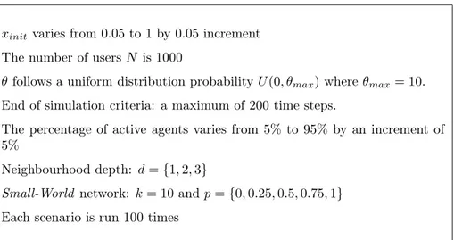
• xinit varies from 0.05 to 1 by 0.05 increment
• The number of users N is 1000
• θ follows a uniform distribution probability U(0, θmax)where θmax= 10.
• End of simulation criteria: a maximum of 200 time steps.
• The percentage of active agents varies from 5% to 95% by an increment of 5%
• Neighbourhood depth: d = {1, 2, 3}
• Small-World network: k = 10 and p = {0, 0.25, 0.5, 0.75, 1} • Each scenario is run 100 times
Table 2: Simulation scenarios resume
Analytical Results
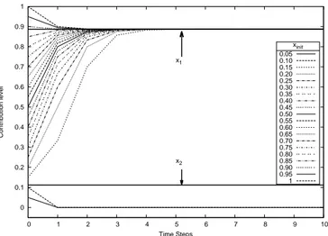
The solution of the analytical model yields a fixed-point dynamics with the attractors x1 = 0.88729833 and x2 = 0.11270167. This means that the
contribution level stabilizes at 88.7% when the initial contribution level xinit
is higher or equal to 11.2%, and that the contribution level will drop to zero if the initial contribution level xinit is lower than 11,2%. Figure 1 illustrates
the expected behaviour, according to this solution.
In the figures describing the simulation results, the attractors x1 and
x2 predicted by the analytical model are identified where necessary with a
horizontal and vertical line, accordingly. Each point represents the mean observed value after having executed 100 times the simulation of the model. We present as well in the figures the minimum and maximum values observed during the simulations.
Iterated model
The experiments reproduced the results predicted by the analytical model nearly all the times. In some of the experiments, around the attractor x2,
the final contribution level was not the one expected. This can be observed in figure 2a. We suppose that this is due to rounding errors. So, we consider that the system behaves in the same way as the analytical model predicts but within an error range resulting from the numerical simulation.
Asynchronous model
In the experiments done with this model, the proportion of active agents at each time step varied from 5% to 95%, in steps of 5%.
0 0.1 0.2 0.3 0.4 0.5 0.6 0.7 0.8 0.9 1 0 1 2 3 4 5 6 7 8 9 10 Contribution level Time Steps x1 x2 xinit 0.05 0.10 0.15 0.20 0.25 0.30 0.35 0.40 0.45 0.50 0.55 0.60 0.65 0.70 0.75 0.80 0.85 0.90 0.95 1
Figure 1: Contribution level evolution as given by the analytical model with θmax = 10and different values of xinit.
It can be seen in figure 2c that, when there are 25% or more active agents in the system, the contribution level dynamics is the same as that of the iterated and analytical models. On the other hand, it can be seen in the figure describing the results of the asynchronous model with a small proportion of active agents (figure 2e) that the smaller the proportion of active agents, the more the final value will be close to 80%, which is less than the value of x1 of the analytical model. In the inset of figure 2e, we
can see that if the value of xinit is lower than 0.88, the value of xf seems to
approach asymptotically x1. Also in the inset, we can see that if the value
of xinit is higher than 0.88, xf approaches asymptotically 0.88, remaining
higher than 0.88.
Topological model
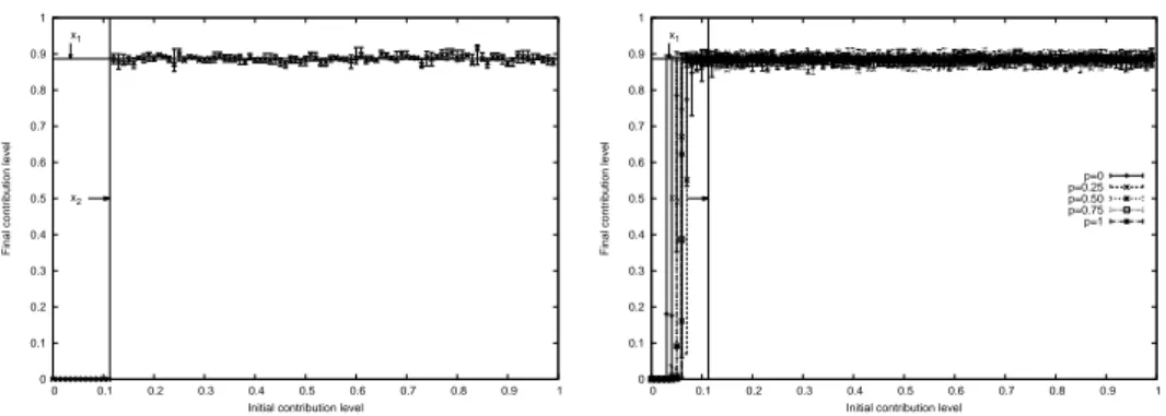
With the topological model, the experiments consisted of varying, on one hand, the depth degree d of the neighbours used by each agent to estimate the cost of sharing, and on the other hand, the probability p that makes the network structured, Small-World or completely random. The values used for d are 1,2 and 3 and the ones for p are {0,0.25,0.50,0.75,1}. We present here only the results for d = 1 and d = 3 in figures 2b and 2d respectively because they are sufficiently representative. For the network configured as a circular lattice (p = 0) the final contribution level starts to stabilize to a value higher than zero at values of xinit higher than 3% for d = 1 and
higher than 5% for d = 3. For the other configurations of p > 0, the stabilization of the contribution level to a value greater than zero starts at around 5%. For all these cases, the stabilization values greater than zero obtained when xinit< 7%are not close to the value of the attractor x1. Yet,
it should be noticed that for a depth degree d = 3, the system exhibits the same behaviour as that of the iterated model except for the case where the network is configured as a circular lattice (p = 0). This can be observed in figure 2d. Further, it should be noticed that, for the values of d = 1 and d = 3, when p = 0 the contribution level starts to stabilize at values higher than zero, sooner (in terms of xinit) than when p > 0. This can be seen
in figures 2b and 2d. Also, it can be seen in the same figures, that when the users have a poor perception of the global contribution level (d = 1), the system will start to stabilize to a value other than zero (that is, will not collapse) at a proportion of sharing peers lower than that predicted by the analytical model.
Asynchronous and topological model
For the experiments done with this model, the values of d varied among 1,2 and 3, and also the values for the proportion of agents active at each time step varied from 5% to 95% in steps of 5%. We present only the results of the simulations for d = 1 in figure 2f since they are sufficiently representative of the other values of d.
As depicted in figure 2f , the final contribution level xf becomes zero
when the proportion of active agents per time step is lower than 25%. It can also be seen in the figures that when the initial contribution level is greater than 25%, the contribution level stabilizes at values around 80% when the proportion of active agents per time step is near 95%.
It shall also be noticed that:
• in figure 2c the asynchronous model with 25% of active agents stabilizes at the value predicted by the analytical model.
• in figure 2b the topological model (with 100% of active agents) stabi-lizes at the value predicted by the analytical model,
• in figure 2f the asynchronous and topological model with 50% and 75% of active agents per time step stabilizes at values between 35% and 65%, far from those predicted by the analytical model.
Finally, we observed in the experiments conducted with the asynchronous and topological model, that when the network has a structure that is close to random (that is, as p grows to values near 1), the stabilization values will be higher, in regard to the proportion of agents active per time step.
Discussions
The question motivating our study was to evaluate the implications of addi-tional time and space dimensions, in regard to the behaviour of the system
0 0.1 0.2 0.3 0.4 0.5 0.6 0.7 0.8 0.9 1 0 0.1 0.2 0.3 0.4 0.5 0.6 0.7 0.8 0.9 1
Final contribution level
Initial contribution level
x2
x1
(a) Iterated model. Mean, minimum and
maximum values of the final contribution level. 0 0.1 0.2 0.3 0.4 0.5 0.6 0.7 0.8 0.9 1 0 0.1 0.2 0.3 0.4 0.5 0.6 0.7 0.8 0.9 1
Final contribution level
Initial contribution level
x2 x1 p=0 p=0.25 p=0.50 p=0.75 p=1
(b) Topological model. Mean, minimum
and maximum values of final contribution for depth d = 1. 0 0.1 0.2 0.3 0.4 0.5 0.6 0.7 0.8 0.9 1 0 0.1 0.2 0.3 0.4 0.5 0.6 0.7 0.8 0.9 1
Final contribution level
Initial contribution level
x2 x1 Active Agents 25% 50% 75% 95%
(c) Asynchronous model. Mean, minimum and maximum values of the final contribution level with 25 %, 50 %, 75 % and 95 % of active agents. 0 0.1 0.2 0.3 0.4 0.5 0.6 0.7 0.8 0.9 1 0 0.1 0.2 0.3 0.4 0.5 0.6 0.7 0.8 0.9 1
Final contribution level
Initial contribution level
x2 x1 p=0 p=0.25 p=0.50 p=0.75 p=1
(d) Topological model. Mean, minimum and maximum values of final contribution for depth d = 3. 0 0.1 0.2 0.3 0.4 0.5 0.6 0.7 0.8 0.9 1 0 0.1 0.2 0.3 0.4 0.5 0.6 0.7 0.8 0.9 1
Final contribution level
Initial contribution level
x2 x1 Active Agents 5% 10% 15% 0.8 0.85 0.9 0.95 1 0.75 0.8 0.85 0.9 0.95 1 x1
(e) Asynchronous model. Mean, minimum
and maximum values of the final contribution level with 5 %, 10 % and 15 % active agents.
0 0.1 0.2 0.3 0.4 0.5 0.6 0.7 0.8 0.9 1 0 0.1 0.2 0.3 0.4 0.5 0.6 0.7 0.8 0.9 1
Final contribution level
Initial contribution level
x2 x1 Active Agents 10% 25% 50% 75% 95%
(f) p = 0,75. Asynchronous and topological model. Mean, minimum and maximum values of the final contribution level with depths d = 1 with 10%, 25%, 50%, 75% and 95% active agents.
Figure 2: Experimental results of the multi-agent models.
(which in turn is the object of study of our models). It is possible to answer to the question according to two different points of view.
The first one is the quantitative behaviour of the system, that is, is the network stable at the same proportion of sharing peers, no matter which model is used? The second one is concerned with the qualitative behaviour. It can consider different aspects such as: is the system active or has it col-lapsed? Is the system stabilizing (at different proportions of sharing peers, depending on the model)?
In the following sections we intend to answer these questions, using the models when possible or using the experimental results.
A priori equivalence conditions of the models
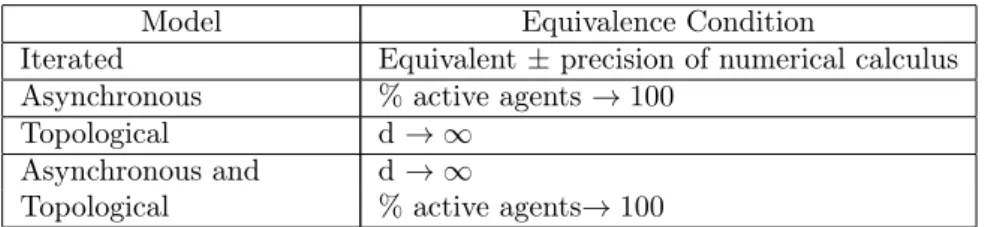
A starting point to compare the different models, is identifying the a priori equivalence conditions under which the models should agree in their answers. Table 3 shows a resume of the equivalence conditions.
Model Equivalence Condition
Iterated Equivalent ± precision of numerical calculus Asynchronous % active agents → 100
Topological d → ∞ Asynchronous and d → ∞
Topological % active agents→ 100
Table 3: A priori equivalence conditions of the models. The multi-agent models can a priori, under certain conditions reproduce the results of the analytical model. Conversely, this table emphasizes that the analytical model can not reproduce a priori the whole spectrum of results of the multi-agent models.
If we use the iterated model, we can expect to see the same results as those of the analytical model, plus the error induced by the numerical calculus.
In the case of topological model, there can be two kinds of equivalence when an agent has a perfect global knowledge of the contribution level: if an agent can interact with all the other agents and if an agent can estimate the contribution level at the maximal depth possible
From a broader perspective, the higher the depth or the more the graph is completely connected, the more the results should be close to those of the iterated or analytical models.
The asynchronous model is equivalent to the iterated or analytical model if all the agents decide to share or not at the same time step. We can assert from a broader perspective that the more the proportion of agents are active at a time step, the more the results will be close to those of the analytical or iterated model.
Finally, the asynchronous and topological model needs to fulfil two con-ditions at the same time to be equivalent with the other models: on the one hand, a big proportion of agents must be active at each time step, and on the other hand, the agents should be able to interact with a lot of other agents.
These equivalences are confirmed by our experimental results.
Comparison of the models in terms of the experimental results
The simulation results show that, although we could identify equivalences between the models in some cases, they only appear under certain conditions. For example, both the asynchronous model and the topological model show the same qualitative behaviour as the analytical or iterated model when xinit ≥ x2 (stabilisation at a fixed value), but it is not the same case when
xinit< x2 (there is no systematic collapse of the system). The asynchronous
and topological model has the inverse behaviour: it agrees with the analytical and iterated models when xinit < x2 (collapse) but when xinit ≥ x2, it
stabilizes with a certain deviation around the final stabilisation value. Another point of view to consider is the resolution time. With the ana-lytical model, we have an immediate answer to the question of the dynamics of the phenomenon without needing to feed it with the amount of users in the system, provided a solution to the model is available. This is not the case with the multi-agent models, where we are forced to give values to the parameters of the model before simulating. In our study case, this implies, for instance, to have an estimation of the amount of users in the system, the kind of network, the rate of connection and disconnection or their up-date frequency. Moreover, the behaviour of the system will be obtained by aggregating the individual values of the contribution level.
Given that we have some equivalences, it is possible to determine which model to use, depending on initial conditions. Specifically, we could say that for the models that give answers similar to those of the analytical and iterated models when xinit≥ x2, we do not have to run simulations to know
which is going to be the final stabilisation value, and even less, to specify the initial parameters (namely, those of the graph building algorithm).
Nonetheless, if we are interested in the process that leads to the results, or in the variability of the final values, only the multi-agent models allow to answer to this question.
Generally speaking, the multi-agent models are richer than the analytical model because they allow to modify the time during which the users are in action, and also, they allow to modify the space in which they find themselves and thus their perceptions of the environment. Hence, they are easier to be used to answer to a whole family of questions holding some wide hypotheses. Therefore, passing from the model proposed by (Feldman et al., 2006), to a model where generosity follows a distribution other than uniformity, is easy with the multi-agent models, but can be complicated with the analytical
model.
Conclusion
This report studies the influence of the integration of time and space dimen-sions when modelling a collective phenomenon. We compared five different models of the free-riding phenomenon where the individual decision mecha-nism remains unchanged while different hypotheses about the modelling of time and space are made. We have demonstrated that such hypotheses can produce contradictory results. We claim that care must be taken when mod-elling and simulating collective phenomena. In particular, attention must be paid when using multi-agent models, that include time and space dimen-sions. The hypotheses made about these dimensions have an influence on the answers given by the model.
Moreover, this may be the case both at the qualitative level and at the quantitative level, as shown by the results obtained with the asynchronous and topological model. We found equivalence criteria between the models, as well as value ranges under which a model with a global point of view (an-alytical model) can be used to answer questions regarding local parameters. Multi-agent models are well suited for modelling collective phenomena be-cause they include both, the individual level of description, and the global. This is an advantage over analytical models that directly describe the global behaviour because they allow to study the influence that local interactions have over the global behaviour of the system. Nonetheless, when using a multi-agent model, special attention must be paid to the way the time and space dimensions are defined in it. If the hypotheses made regarding those dimensions are not fully stated, the range of applicability of the answers given by the model may be uncertain. Our work shows also that analytical models and individual-based models may be complementary (Grimm and Railsback, 2005). In our results, we find (generally speaking) two attractors in the dynamics of the system (either the contribution level stabilizes, or it becomes zero). However, the analytical model cannot specify the exact value of the attractors (nor its variability) for each of the network configurations, no matter if it includes the time or the space dimensions (local characteristics integration). Also, it cannot describe the process underlying the dynamics but it captures the essence of the dynamics (stabilisation).
In a broad sense, our work in centred around knowing the validity do-mains of a group of models. That is, to know under which limits the results given by a model can be considered as useful. This question is unavoidable and very important when the model is to be used beyond the comprehension of the phenomenon it represents: for instance, when the model outcomes are used as predictions of the behaviour of the system for regulation purposes.
Bibliography
Adar, E. and Huberman, B. A. (2000). Free riding on gnutella. First Monday, 5(10). [online].
Axtell, R. (2001). Effects of Interaction Topology and Activation Regime in Several Multi-Agent Systems. In Moss, S. and Davidsson, P., editors, Multi-Agent-Based Simulation, volume 1979 of Lecture Notes in Computer Science, pages 33–48. Springer Berlin / Heidelberg. 10.1007/3-540-44561-7_3.
Caron-Lormier, G., Humphry, R. W., Bohan, D. A., Hawes, C., and Thorbek, P. (2008). Asynchronous and synchronous updating in individual-based models. Ecological Modelling, 212(3-4):522–527.
Chevaillier, P., Bonneaud, S., Desmeulles, G., and Redou, P. (2009). Ex-perimental Study of Agent Population models with a Specific Attention to the Discretization Biases. In Proceedings of the European Simulation and Modelling Conference, ESM’09, EUROSIS, The European Simulation Society. AI-Akaidi, M. (ed.), pages 323–331. The European Simulation Society.
Cornforth, D., Green, D. G., and Newth, D. (2005). Ordered asynchronous processes in multi-agent systems. Physica D: Nonlinear Phenomena, 204:70–82+.
Costa-Montenegro, E., Burguillo-Rial, J., Rodriguez-Hernandez, P., Gonzalez-Castano, F., Curras-Parada, M., Gomez-Rana, P., and Rey-Souto, J. (2008). Multi-Agent System Model of a BitTorrent Network. In Software Engineering, Artificial Intelligence, Networking, and Paral-lel/Distributed Computing, 2008. SNPD ’08. Ninth ACIS International Conference on, pages 586–591.
Delgado, J. (2002). Emergence of social conventions in complex networks. Artificial Intelligence, 141(1-2):171–185.
Fatès, N. and Chevrier, V. (2010). How important are updating schemes in multi-agent systems? An illustration on a multi-turmite model. In Pro-ceedings of the 9th International Conference on Autonomous Agents and
Multiagent Systems, volume 1, pages 533–540. International Foundation for Autonomous Agents and Multiagent Systems.
Feldman, M., Papadimitriou, C. H., Chuang, J., and Stoica, I. (2006). Free-riding and whitewashing in peer-to-peer systems. IEEE Journal on Se-lected Areas in Communications, 24(5):1010–1019.
Ferber, J. (1999). Multi-Agent Systems: An Introduction to Distributed Ar-tificial Intelligence. Addison-Wesley.
Ge, Z., Figueiredo, D., Jaiswal, S., Kurose, J., and Towsley, D. (2003). Mod-eling peer-peer file sharing systems. In IEEE INFOCOM 2003. Twenty-Second Annual Joint Conference of the IEEE Computer and Communica-tions Societies.
Goldstone, R. and Janssen, M. (2005). Computational models of collective behavior. Trends in Cognitive Sciences, 9(9):424–430.
Grimm, V. and Railsback, S. (2005). Individual-based modeling and ecology. Princeton Univ Pr.
Hong, T. (2001). Performance. In Oram, A., editor, Peer-to-Peer Harnessing the Power of Disruptive Technologies, chapter 14, pages 203–241. O’Reilly Media.
Hua, J.-S., Huang, S.-M., Yen, D. C., and Chena, C.-W. (2011). A dynamic game theory approach to solve the free riding problem in the peer-to-peer networks. Journal of Simulation.
Huberman, B. A. and Glance, N. S. (1993). Evolutionary games and com-puter simulations. Proceedings of the National Academy of Sciences of the United States of America, 90(16):7716–7718.
Jian, L. and MacKie-Mason, J. (2008). Why share in peer-to-peer networks? In Proceedings of the 10th international conference on Electronic com-merce. ACM New York, NY, USA.
Jovanović, M., Annexstein, F., and Berman, K. (2001). Modeling peer-to-peer network topologies through small-world models and power laws. In IX Telecommunications Forum, TELFOR.
Kittock, J. (1993). Emergent conventions and the structure of multi-agent systems. In Proceedings of the 1993 Santa Fe Institute Complex Systems Summer School. Citeseer.
Macal, C. and North, M. (2010). Tutorial on agent-based modelling and simulation. Journal of Simulation, 4(3):151–162.
Minsky, M. (1965). Matter, Mind and models. In Proceedings of International Federation of Information Processing Congress, volume 1, pages 45–49. Miralles, J. C., López-Sánchez, M., and Esteva, M. (2009). Multi-agent
system adaptation in a peer-to-peer scenario. In Proceedings of the 2009 ACM symposium on Applied Computing, SAC ’09, pages 735–739, New York, NY, USA. ACM.
Mitchell, M., Thomure, M., and Williams, N. (2006). The Role of Space in the Success of Evolutionary Learning. In Artificial life X: proceedings of the Tenth International Conference on the Simulation and Synthesis of Living Systems, volume 10, page 118. The MIT Press.
Parunak, H., Savit, R., and Riolo, R. (1998). Agent-Based Modeling vs Equation-Based Modeling: A Case Study and Users’ Guide. Lecture Notes in Computer Science, 1534:10–25.
Phan, D. and Amblard, F., editors (2007). Agent-based modelling and simula-tion in the social and human sciences. GEMAS Studies in Social Analysis. Bardwell.
Ramaswamy, L. and Liu, L. (2003). Free riding: A new challenge to peer-to-peer file sharing systems. In Proceedings of the Hawaii International Conference on Systems Science, page 220.
Sen, O. and Sen, S. (2010). Effects of Social Network Topology and Options on Norm Emergence. In Padget, J., Artikis, A., Vasconcelos, W., Stathis, K., da Silva, V., Matson, E., and Polleres, A., editors, Coordination, Or-ganizations, Institutions and Norms in Agent Systems V, volume 6069 of Lecture Notes in Computer Science, pages 211–222. Springer Berlin / Heidelberg.
Shoham, Y. and Tennenholtz, M. (1997). On the emergence of social con-ventions: modeling, analysis, and simulations. Artificial Intelligence, 94(1-2):139–166.
Stutzbach, D., Rejaie, R., and Sen, S. (2008). Characterizing unstructured overlay topologies in modern P2P file-sharing systems. IEEE/ACM Trans-actions on Networking, 16(2):267–280.
Vassilakis, D. and Vassalos, V. (2007). Modelling real p2p networks: The effect of altruism. In Seventh IEEE International Conference on Peer-to-Peer Computing, 2007. P2P 2007, pages 19–26.
Villatoro, D., Sen, S., and Sabater-Mir, J. (2011). Exploring The Dimensions Of Convention Emergence In Multiagent Systems. Advances in Complex Systems, 14(2):201–227.
Watts, D. and Strogatz, S. (1998). Collective Dynamics of ’small-world’ networks. Nature, 393:440–442.
Yusuke, M., Masahiro, S., and Tetsuya, T. (2010). Evolutionary Game Theory-Based Evaluation of P2P File-Sharing Systems in Heterogeneous Environments. International Journal of Digital Multimedia Broadcasting, 2010.