HAL Id: hal-02963404
https://hal.archives-ouvertes.fr/hal-02963404
Submitted on 10 Oct 2020HAL is a multi-disciplinary open access
archive for the deposit and dissemination of sci-entific research documents, whether they are pub-lished or not. The documents may come from teaching and research institutions in France or
L’archive ouverte pluridisciplinaire HAL, est destinée au dépôt et à la diffusion de documents scientifiques de niveau recherche, publiés ou non, émanant des établissements d’enseignement et de recherche français ou étrangers, des laboratoires
Proton exchange membrane fuel cell behavioral model
suitable for prognostics.
Elodie Lechartier, Elie Laffly, Marie-Cécile Péra, Rafael Gouriveau, Daniel
Hissel, Noureddine Zerhouni
To cite this version:
Elodie Lechartier, Elie Laffly, Marie-Cécile Péra, Rafael Gouriveau, Daniel Hissel, et al.. Proton exchange membrane fuel cell behavioral model suitable for prognostics.. International Journal of Hydrogen Energy, Elsevier, 2015, 40 (26), pp.8384 - 8397. �hal-02963404�
Proton Exchange Membrane Fuel Cell behavioral model
suitable for prognostics
Elodie Lechartiera,b, Elie Lafflyc, Marie-C´ecile P´eraa,b, Rafael Gouriveaua,b, Daniel Hissela,b, Noureddine Zerhounia,b
aFEMTO-ST Institute (UMR CNRS 6174) 24 rue Alain Savary, 25000 Besancon, France bFCLAB (FR CNRS 3539),rue Thierry Mieg, 90000 Belfort FRANCE
cAlstom Hydro, 3 av des Trois Chenes, 90000 Belfort FRANCE
Abstract
Prognostics and Health Management (PHM) is a discipline that enables the estimation of the Remaining Useful Life (RUL) of a system and is not yet much applied to Proton Exchange Membrane Fuel Cell PEMFC. How-ever it could permit the definition of adequate conditions allowing extending PEMFC’s too short life duration. For that purpose, a model that can repro-duce the behavior of a PEMFC is needed. This paper presents a model of a PEMFC that could serve for a prognostics purpose. The model is composed of a static part and a dynamic parts that are independent. On one side, the static part is developed thanks to equations describing the physical phenom-ena and is based on the Butler-Volmer law. On the other side, the dynamic part is an electrical equivalency of physical phenomenon. The models are validated thanks to experimental data gathered in long term tests. For that purpose the parameters are successively updated based on characterization measurements (polarisation curves and EIS (electrochemical impedance spec-troscopy)). Then the results of the model are compared to the ageing data in order to evaluate if the model is able to reproduce the behavior of the fuel cell. The usefulness of this model for prognostics is finally discussed.
Keywords: Proton Exchange Membrane Fuel Cell, Prognostics and Health Management, Behavioral Model, Static, Dynamic,
Nomenclature
ηa Voltage drop at the anode [V ]
ηc Voltage drop at the cathode [V ]
τOc Time constante of the diffusion convection impedance [s]
ba Tafel anode parameter V−1
bc Tafel cathode parameter [V−1]
bOc Parameter of the variation law of ROc [V−1] Cdca Double layer capacity at the anode [F/cm2] Cdcc Double layer capacity at the cathode [F/cm2]
En Nernst Potential [V ]
i Number of EIS realized at each characterizations
j0a Exchange current density at the anode [ A/cm2]
j0c Exchange current density at the cathode [ A/cm2]
j0Oc Parameter of the variation law of ROc [A/cm2]
JAC Dynamic current density [A/cm2]
JDC Static current density [A/cm2]
JEIS Vector of the current densities for the EIS [A/cm2] Jpola Vector of the current densities for the polarization curve [A/cm2]
jLc Limit current density at the cathode [A/cm2] k Number of characterizations
kOc Parameter of the variation law of τOc [A.s/cm2]
L Connectors’ inductance [H.cm2]
Rm Membrane resistance [Ω.cm2]
r Internal resistance (Static and Global model) [Ω.cm2]
ROc Module of the diffusion convection impedance [Ω.cm2] Rta Transfert resistance at the anode [Ω.cm2] Rtc Transfert resistance at the cathode [Ω.cm2]
U Stack Voltage [V ]
UAC Dynamic stack Voltage normalised per cell [V ] UDC Static stack Voltage normalised per cell [V ]
Un Stack voltage normalized per cell [V ] WOc Diffusion convection impedance [Ω.cm2]
1. Introduction
PEMFC is a promising alternative to the actual production of energy but has got technical bolts as the distribution and the storage of dihydrogen as
well as a too short life duration [1]. In order to postpone the end of life, the development of Prognostics and Health Management (PHM) seems to be an adapted solution. The part of PHM that is highlighted here and that has not been investigated much in literature is Prognostics. The idea is to estimate the Remaining Useful Life of a system. For that purpose, as a starting point, a behavioral model, including ageing, of a PEMFC is needed. For modeling the behavior, different kinds of approaches can be highlighted, like data-based [2] or model-based [3], both largely present in the literature. However, neither of these models seems to fit the diagnostics purpose. Indeed, for examples, the ageing phenomena can hardly be added if only the micro phenomenon happening in the fuel cell are modeled [4]. For that purpose, a model-based approach is developed in this paper in order to have a good precision and even to model some important internal parameters of the fuel cell. A combination of a static and a dynamic model is proposed and fulfills the need of a model in an efficient way. Indeed, added to the positive aspects of a model-based approach, this model is rather easy to implement, has a high enough accuracy with the description of internal parameters, and the ageing can be easily included.
This paper is structured as follows. First a presentation of the path made toward a behavioral model usable for prognostics is drawn, then the model developed is presented. Next the updating procedure, i.e. the tuning of parameters’ values is explained for finally studying the validation thanks to the comparison between the simulated behavior and experimental results.
2. Backgrounds
2.1. Prognostics and Health Managment (PHM)
Every machine or system is deteriorating with time until reaching a faulty state. It can happen at an unsuitable time and trigger negative consequences as it prevents the system to ensure its mission. The maintenance could take a lot of time, and meanwhile, all the dependent systems are not able to carry on. Some loss of money or time and even security troubles can be triggered by this situation. PHM appears to be a solution to face this kind of problems [5]. Among the aims of PHM, the principals are:
• To improve the decision making process in order to increase the life
duration of the system;
• To improve the security of the system.
PHM is described as composed of seven modules (figure 1) that allow defining the different steps followed in the process [6] . With a first part of obser-vation composed by the data acquisition (module 1) obtained thanks to the sensors and by the data processing (module 2) which allows extracting some features. Then the analysis part is composed by modules 3, 4 and 5. Mod-ule 3 (condition assessment) aims defining the state of health of the system by detecting faults. Then, the module 4, diagnostic, assesses the origins of the faults. Module 5, prognostics, predicts the future state of health of the monitored system thanks to previous modules. It allows estimating the re-maining useful life (RUL). The action part of PHM is composed by the last two modules. First, the decision support provides recommendations about the actions that should be taken to fulfill the mission while optimizing crite-ria like cost or time to failure. And then, the human-machine interface that allows the communication with the user but also the overall link between the modules.
2.2. PHM of fuel cell
Even though the PHM, under its denomination, has not been applied a lot to the fuel cell, but papers dealing with the different modules of PHM can be found in the literature. For example different authors [8, 9, 10, 11, 12, 13] develop the modules of the observation part and even diagnostics [12, 13, 14, 15, 16]. There is a lot of paper already dealing with diagnostics for the PEMFC and the previous steps. However, there are only few paper dealing with the step further which is PEMFC pronostics [17], on which focus this paper.
The ISO definition of prognostics is: “estimation of the operating time before failure and the risk of existence or later appearance of one or more failure modes”. It allows defining the Remaining Useful Life (RUL) that is according to the ISO standard [18] : “estimation of the time past between the current moment and the moment when the monitored machine is considered as failed”. So, prognostics aims at predicting the time left for the system to be functional. In this objective, approaches for prognostics [19] can be distinguished as follows:
• Data-driven [20, 21, 22] approaches aim at approximating and
predict-ing the behavior of the system thanks to experimental data and without an analytical model of the underlying phenomena. Those approaches are usually performed thanks to machine learning tools like neural net-work. This kind of approaches is generally simple to implement but has no link with the internal phenomenon. It is then not possible to correlate the state of health observed or predicted with the real physic happening. These approaches are effective if a large amount of data is available, which is not always the case.
• Model-based approaches are based on the description of the physical
phenomena happening. Equations developed thanks to a precise study of the behavior based on global knowledge as for exemple, chemistry or electronics is the startpoint of this approach. Indeed, the failure criteria developed in this approach are the description of the failure mechanisms by explicit mathematical representation. This approaches are reliable but require a precise knowledge of the physics phenomenon happening in order to be able to model it.
• Hybrid approaches are based on the two last approaches. The idea is,
accurate and reliable result. Effort has to be made to avoid a two high computational cost and to reach a satisfying applicability.
The classification of the physic-based approach can be discussed. In-deed, even though the model is based on the description of the physical phenomenon, data are needed in order to obtain appropriate parameters of the model.
The models of PEMFC that can be found in the literature cover different approaches from physic-based to data-based. Data driven approaches won’t model any physic phenomenon and will need a significant amount of data for the learning phase. They can be represented as black boxes [20]. They presents more or less the same drawbacks than the data-driven approach of prognostics and don’t comply with our needs. Then it was chosen to study only the physical-based as this kind of approaches has not been developed yet for our purpose but also because it would allow keeping a strong link with the actual physical phenomenon. The physic-based model describe the physic phenomenon happening. Some are formalized thanks to an electrical equivalency [23, 24, 25, 26], while others directly exploit the physical and chemical equations [27, 28, 29, 4, 30].
The black box modeling has already been investigated [21, 31]. The physical based approach is developed with this first step of modeling.It would allow gaining in precision and even adding some possible analysis as some internal parameters with a physical meaning are represented. In this work, we choose to develop a physics-based approach applied on a PEMFC stack as the stack is defined as the object of the study (excluding the other components of the PEMFC system).
3. Literature review: Towards an analytical behavior model
Numerous works has been analyzed in order to define and identify a model that would comply with the PHM needs. A synthesis is shown thanks to the table 1.
3.1. Aims of the models
The goal of the model should be convenient for a prognostics use. A comprehensive model could be usable, but the development should present a capacity of adaptation as allowing the addition of a new input without too much burden. A model for comprehensive purpose is a model which
aims understanding the interaction between different electrochemical mech-anisms. The claimed objectives are variables: Fouquet et al. [23] developed their model for diagnostic purpose, while Siegel et al. [27] objective is com-prehension whereas for Hinaje et al. [32] it is a development that would allow the control. In other references, the underlying aim is not always given, even if it is a capital fact, as a model developed for purpose of design [33] won’t fit most of the time for another application.
3.2. Boundaries of the model
The boundaries of the expected model are the terminal of the stack as it is the stack’s RUL which is here investigated. The modeled objects differ also among the papers. The ones that model the whole system or a part of it [34] haven’t been retained as it is beyond the scope of this study. Some models concern a single cell [4, 24, 27, 28, 29, 32]. Fouquet et al [23] use a model of a single cell, and extend it for modeling a stack. It is the same for Shan et al. [35] that presents a cell model and then use it for modeling a stack. So, some models of single cell can match with our needs, if they can be extended to a stack, implying a few assumptions or modifications. Finally some authors model directly stacks [3, 25, 36].
3.3. Static or dynamic models
A static model would be convenient as the objective is to model the behavior for a long time scale under a constant load in a first step. But a dynamic model would be convenient as it brings more precision on the behavior’s description and would make the model more reliable under variable load. However it is an open question. Defining a model as static or dynamic is not an easy task. Indeed, there is no clear agreement in the literature about a definition. A model with a time dependency can be considered as dynamic regardless to the value of the time constant, while for some authors a model with a low time constant is a static model. Thus, some models are are labeled as dynamic as [4, 25, 30, 35] whereas other as static [23] but not always with the same definition. However a lot of authors don’t even define the nature of their model, and some can appear static [24, 27] or dynamic [36] with the analysis of their work face to our definition.
3.4. Space and time scale
The space scale of the phenomenon described in the models is also variable as well as the dimension of the model. A thin granularity, down to the
nanometer, is often linked to a high dimension description and suits more the design purposes. A review of this kind of models is available [37], with detailed models of precise phenomena. For prognostics purposes, a 1D or even 0D model should be precise enough and have a compatible computing cost [23, 24, 27, 28, 29, 36]. Furthermore, the time scale of the phenomena retained in the description doesn’t need to be low as thousands of hours as simulated time might be necessary to forecast the RUL. However, the fastest phenomena can be kept then neglected in a second step if necessary.
3.5. Degradation already included in the model
As our final final need is to model the ageing, a model that includes some degradation would present advantages. For example Fouquet et al. [23] characterize the flooding and drying of the membrane in order to classify the degraded operating modes of the fuel cell. Lee et al. [24] as well as Laffly [38] did try to model the ageing by fitting parameters’ evolution with polynomial function. In their work, Robin et al. [3] tried to model the Pt surface degradation mechanism.
3.6. Validation of the models
The model should have been validated with experiments to be reliable enough.
The validation strategies are variable too, as some authors validate their models thank to experimentations [33, 36], some others thanks to comparison done with other publication [39], or even with equations solver results [32]. Lee et al. [24] validate their model by evaluating the fitting of their curve with the real data, it means that it is the evaluation of the parameters and the shape of the model that are validated on the example not its predictive ability. Hou et al. [36] evaluate the parameters thanks to experiments and then, validate them thanks to another test on another stack.
3.7. Synthesis and discussion
Table 1 presents the characteristics of each model versus all the criterion. At the first sight, on table 1, some model appear to fulfil the criteria but a deeper analysis is needed:
1. The model of Robin et al. [3] presents a combination of an analyti-cal model and a semi-empirianalyti-cal one. A degradation : the Pt surface degradation is included in this model. But the need of the local partial pressure is a strong limitation of this model.
2. The model of Fouquet et al. [23] is an electrical equivalent circuit that is based on Randles model but improved with a Constant Phase Element. However in this model the two electrodes are not separated, which decreases the level of information.
3. The model of Reggiani et al. [25] is a model based on an electrical equivalent circuit. This model doesn’t present enough precision for the purpose here as the model proposed doesn’t go really deep in the the phenomenon modeled, for example, there is not differentiation between anode and cathode. The gain of using a physics-based approach would not be as great as expected because the hypothesis of simplification are pushed too far.
4. The model of Hou et al. [36] is a model that has an objective re-ally focused, indeed, models for the voltage overshoot and undershoot are developed here. So these models are not complete enough for the purpose of this paper.
As no model that could be found in literature complies with each criterion (table 1), a new model is presented in this paper that is more adapted to our need of prognostics purpose.
4. Behavioral model description
4.1. Overall presentation
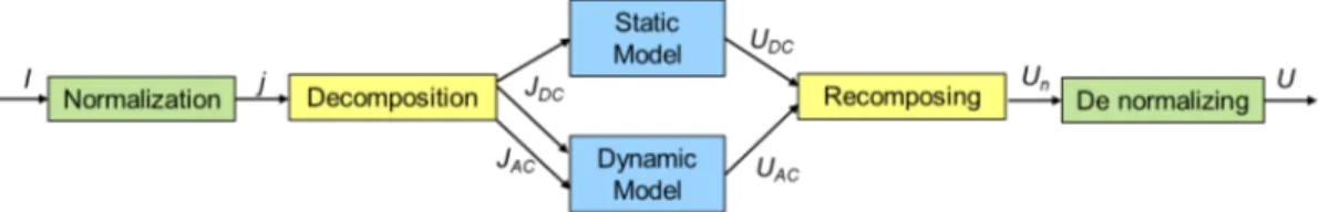
The proposed behavioral model is depicted in figure 2. The only input of this model is the current which is then normalized in the current density to be decomposed in direct and alternating current densities thanks to a low pass filter. These current densities are then used as the inputs of the models in order to furnish the output that are direct and alternating voltage per cell which are finally recomposed in voltage per cell to be denormalized in voltage.
First Model Object Static or
Ref. author type Aim modeled dynamic Degradation Physical &
[3] Robin chemical desc. Comprehensive Stack Dynamic Modeled Phys. & chem.
[39] Asl des. & electrical Not clearly Stack Dynamic No eq. circuit defined
Electrical
[23] Fouquet equivalent Diagnostic Cell Dynamic Characterized
circuit → stack (Classified)
Electrical
[24] Lee eq. circuit Diagnostic Cell Static Modeled Electrical Not clearly
[25] Reggiani eq. circuit defined Stack Dynamic No Electrical Not clearly Cell
[26] Lazarou eq. circuit defined → stack Dynamic No Physical &
[27] Siegel chemical des. Comprehensive Cell Static No Physical & Not clearly
[28] Martins chemical des. defined Cell Static No Physical &
[29] Chevalier chemical des. Diagnostic Cell Static Modeled Physical & Not clearly
[4] Ceraolo chemical des. defined Cell Dynamic No Physical & Not clearly Cell
[30] Philipps chemical des. defined → stack Dynamic No Phys. & chem.
[32] Hinaje des. & electrical Control Cell Dynamic No eq. circuit
Phys. & chem.
[33] Park des. & electrical Conception Cell Dynamic No
eq. circuit → stack
Physical & Cell
[35] Shan chemical des. Conception → stack Dynamic No Logarithmic
[36] Hou & semi- Not clearly Stack Dynamic No empirical defined
The objective of a prognostic approach is to be able to reproduce the behavior of the system in order to obtain information estimated like the state of health (SOH) or the remaining useful life (RUL). It is in this frame that this model appears to be exploitable for prognostics (figure 3). Indeed, thanks to the model and to ageing data, the prognostic approach can be developed, this would allow providing the informations needed for the next steps of PHM, i.e. the decision process.
Figure 3: Insertion of the model in prognostics
4.2. Static part of the model
The static model based on the Butler-Volmer law is in a first step a vari-ation law that takes into account the activvari-ation phenomenon at the cathode and at the anode by the two voltage drop ηa et ηc.
UDC = En− r · JDC − ηa− ηc (1)
Where r is the internal resistance of the fuel cell, JDC the static current
density and En the Nernst potential.
With the hypothesis that the influence of the hydrogen diffusion can be neglected face to the oxygen ones, the final expression is (2). Indeed during measurements it can be noticed that the diffusion at the cathode has a bigger influence than the diffusion on the anode side [38]. With at the anode and cathode :
• ba, bc the Tafel parameters;
• jLc the limit current density at the cathode only. UDC = En− r · JDC− 1 ba · asinh ( JDC 2· j0a ) − 1 bc · asinh JDC 2· j0c· ( 1− JDC jLc ) (2)
4.3. Dynamic part of the model
Here, the aim is to link the voltage variation to the current variation, with the hypothesis that the variations are around a static operating point.
4.3.1. Summary of the model
The phenomena that are represented in the dynamic model are expressed thanks to an electrical equivalency (figure 4). Indeed, the multi-physical phenomena are represented by electrical impedances with a similar behavior :
• A part of the diffusion convection of the different gases at the cathode
is modeled by a Warburg impedance.
• The double layer capacities at the interface electrode-electrolyte on the
anode and cathode are modeled respectively by capacitor Cdcaand Cdcc. • Two transfer resistances Rta and Rtcrepresent the electrons transfer at
the electrodes.
• The ionic conductance of the membrane is modeled by an equivalent
resistance Rm. A different writing than the internal resistance on the
static part as they are here not linked yet.
• And finally, the inductive behavior due to the connectors is taken into
Figure 4: Electrical equivalency of the dynamic model
4.3.2. Warburg impedance
The Warburg WOc is defined by its module ROc and its time constant τOc
expressed in the Laplace space(eq. (3)).
WOc(p) = ROc·
tanh(√τOc· p) √
τOc· p
(3)
Figure 5: Electrical equivalent circuit of an electrode with a Warburg represented by N RC filter in series
An equivalence for this impedance is a network of n RC filters in series (figure 5). The values of the parameters Rn (eq. (4)) and C (eq. (5)) are as
follows.
Rn =
8· ROc
C = τOc
2· ROc (5)
The equivalent impedance then have for expression (eq. 6), with Rn
developed on (eq. (4)) and Neq the number of RC filters :
WOceq (p) = Neq ∑ n=1 Rn 1 + Rn· C · p (6) When using more than 5 RC filters the error between the model and the measures is under 4%. Yet the experiment measures error have the same order of value, we can consider that 5 filters are enough as up to 5 filters.
4.3.3. State space representation
The equivalent electrical circuit is then expressed thanks to a state space representation in which each electrode has a state space representation. We consider that the current density is well separated in its static JDC and
dy-namic part JAC as they are the different input for the static and the dynamic
model.
A state space representation is expressed as : ˙
X = A· X + B · U (7)
Y = C· X + D · U (8) For the anode (figure 4), with no diffusion convection impedance, the state vector is (eq. (9)) and the matrix of the representation are (eq. (10), (11), (12) and (13)) : X = [IRta] (9) A = [ − 1 Rta· Cdca ] (10) B = [ 1 Rta· Cdca ] (11) C = [Rta] (12) D = [0] (13)
The state space representation at the anode is thus finally (eq. (14)): { [ ˙ IRta ] = [ − 1 Rta·Cdca ] · [IRta] + [ 1 Rta·Cdca ] · [jAC] [UACAnode] = [Rta]· [IRta] (14)
For the cathode, with one diffusion convection impedance, the state vector and the matrix of representation are given bellow on equations (15), (16), (17), (18) and (19). Where Vi is the voltage across the ith RC cell of the
equivalent circuit of the Warburg.
X = V1 V2 · · · VN IRtc (15) A = −1 R1·Ceq 0 · · · 0 1 Ceq 0 R−1 2·Ceq · · · 0 1 Ceq .. . ... . .. ... ... 0 0 · · · R−1 N·Ceq 1 Ceq −1 Rtc·R1·Ceq −1 Rtc·R2·Ceq · · · −1 Rtc·RN·Ceq − N Rtc·Ceq − 1 Rtc·Cdcc (16) B = 0 0 .. . 0 1 Rtc·Cdcc (17) C = [ 1 1 · · · 1 Rtc ] (18) D = [0] (19)
Finally the whole state space representation at the cathode is given by equation (20).
˙ V1 ˙ V2 · · · ˙ VN ˙ IRtc = −1 R1·Ceq 0 · · · 0 1 Ceq 0 R−1 2·Ceq · · · 0 1 Ceq .. . ... . .. ... ... 0 0 · · · R−1 N·Ceq 1 Ceq −1 Rtc·R1·Ceq −1 Rtc·R2·Ceq · · · −1 Rtc·RN·Ceq − N Rtc·Ceq − 1 Rtc·Cdcc · V1 V2 · · · VN IRtc + 0 0 .. . 0 1 Rtc·Cdcc · [jAC ] [UACCathode] = [ 1 1 · · · 1 Rtc ]· V1 V2 · · · VN IRtc (20) 4.4. Global model
As it can be seen on figure 2, the recomposing block is using the two outputs of the static and dynamic model. For the static model, the output
UDC is simply described in equation (2).
For the dynamic model, the expression of UAC can be developed as :
UAC = UACAnode+ UACCathode + UACRm+ UACL (21)
The recomposing block consists in simply adding up the AC and DC of the current density.
5. Model updating procedure
5.1. Global tuning process
In order to validate the model and its capacity to fit with experimental data, but also to confirm its suitability to simulate the behavior of a PEMFC, an estimation of the parameters based on real data is done. Indeed, the objective is to tune the model to actual data, i.e. to adapt the parameters
in order to take into account their evolution due to ageing. This would also enable the model to be applied to different stacks. For that are used the characterization results considered as composed of one polarization curve and i (i = 3 in the reported data) EIS realised at different currents.
The global process can be seen on figure 6. A quick description of the
tuning of the static model and tuning of the static model is proposed here
with a complete development in the two next subsections.
Figure 6: Parameters tuning procedure
On a first step non linear regressions are realized on the i Nyquist plots at the k characterizations. The regressions permit to obtain a first set of the following parameters. As k.i. EIS are used, k.i. values are obtained for each
of these parameters.
• The impedance module ROc and the time constant τOc of diffusion
convection of the oxidant at the cathode
• The double layer capacities at the anode and the cathode Cdca, Cdcc • The transfer resistance at the anode and the cathode Rta, Rtc • The membrane resistance r
• The connector inductance L
Then the tuning of the static model is realized on each polarization curve, the matrix of parameters calculated on the previous step being necessary. This step allows defining the values of the other static parameters (which have not been tuned in the first step and listed below) for each considered characterization :
• Nernst potential En
• Exchange current density at cathode and anode j0c j0a
• Membrane resistance r (that takes the mean value of Rm)
• Tafel parameters at cathode and anode bc ba • Limit current density at the cathode jLc
Next as τOc and ROc depends on the current, the parameters of their time
function are regressed thanks to the current at which the EIS is done. This last tuning will provide for the concerned characterization (and not only for each EIS of this characterization) the following parameters:
• The impedance module ROc and the time constant τOc of the diffusion
convection’s under parameters (j0Oc, bOc and kOc)
• The double layer capacities at the anode and the cathode Cdca, Cdcc • The transfer resistance at the anode and the cathode Rta
• The membrane resistance named r for the global model • The connector inductance L
All of the needed parameters are obtained for tuning the global model. However Rtc’s value has not been defined for the global model. It is also
dependent on the current and the cathode parameters values obtained on the static tuning procedure are used. The expression of Rtc is developed in
equation (22). Rtc = 1 bc · √( 1 JDC 2·j0c·1−jDCjLc )2 + 1 · 1 2· j0c· ( 1−jDC jLc )2 (22)
The parameter values obtained by the update of the static and dynamic model permit to define the model. However, as it is based on a given char-acterization set, the model updated only concerns the evolution around or after the used characterization.
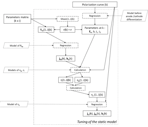
5.2. Tuning of the static model
Here is developed the block update of the static model. A more precise description can be seen on figure 7.
Figure 7: Static model update
For each characterization k, a unique value is necessary for Rm, because
only one is needed on the static equation at each characterization as Rm shouldn’t depend on the current level. The mean of all the values obtained for this parameter at each characterization is thus considered, this parameter is then written r.
The value of Rta at each EIS are already obtained. Yet the transfer
resistance at the anode evolve with the current thanks to the equation (eq. (23) with the exchange current density at the anode j0a and the anode tafel
parameter ba. A regression is then realized with the value of Rta, the values
equation. Rta = 1 ( ba.2.j0a. √( JEIS 2.j0a )2 + 1 ) (23)
Meanwhile, on an other side an other regression is done on the data of the
kthpolarization curve with a model of the fuel cell ”before” the differentiation
anode/cathode (eq. (24)) i.e. the voltage drop is for the whole cell.
Upola = En− r.Jpola− 1 b.asinh Jpola 2.i0. ( 1− Jpola iL ) (24)
All the parameters necessary to obtain the values of the global and an-ode voltage drops are then known. Thanks to their expressions (eq. (25) and (26)) it is now possible to calculate them for all the currents of the polarization curve. η = 1 b.asinh Jpola 2.i0. ( 1− Jpola iL ) (25) ηa= 1 ba .asinh ( Jpola 2.j0a ) (26) From the previous values the cathode voltage drop can be deduced as
η = ηa+ ηc. As the expression of ηc is also know (eq. (27)), a regression on
its values is done in order to obtain the tafel parameter (bc) and the exchange
and limit current density (j0c) at the cathode at this characterization.
ηc= 1 bc .asinh Jpola 2.j0c. ( 1−Jpola jLc ) (27)
With this process, the static model is completely tuned as all the pa-rameters in equation (2) are updated. The model is finally usable after the characterization that allows tuning it.
5.3. Tuning of the dynamic model
The dynamic updating procedure is described on figure 8. For L, Cdca, Cdcc, and Rm the average value is calculated. It is done on all values obtained
at the characterization k considered. Indeed, only one value is needed, taking the i values obtained on the EIS and calculating the mean also permits to smooth if there is errors on the measures.
Figure 8: Dynamic part update
For the development of the diffusion convection parameters, ROc and τOc
some regressions are realized too thanks to their expressions (eq. (28) and (29)). As the i values obtained of the parameters at the characterization k are already known thanks to the very first step of the global tuning process, a regression can be realized. Indeed, their variation laws depend on the current density. For the regression, the current densities at which are realized the i EIS are used.
ROc = 1 ( bOc.2.j0Oc. √( JEIS 2.j0Oc )2 + 1 ) (28) τOc = kOc JEIS (29)
6. Experiments, results and discussion
6.1. Experimental setup
The model is validated thanks to two long-term tests carried out on two different stacks of similar technology (PEMFC composed of 5 cells with an active area of 100cm2).
• A first stack (named FC1) is operated in stationary regime, with a
con-stant load expressed by a current of 70A, at roughly nominal operating conditions during 1000 hours.
• A second stack (named FC2) is operated under dynamic current
test-ing conditions, i.e. with high-frequency triangular current ripples. The current is 70A with a ripple part of more or less 10% at a 5kHz fre-quency. The operating conditions are set constant. The test lasted 1000 hours.
The latter experiment has been realized in order to estimate the per-turbations caused by a power converter usually connected to the fuel cell compared to a constant current in the first experiment. It permits to ensure that the model can still be accurate with the current oscillations caused by the power converter.
For both tests, some values as the voltage, current, or humidity were monitored all along the 1000 hours in order to obtain global historic curves (i.e. evaluating the evolution over time of voltage levels). Besides, character-izations were carried out once per week (around every 160 hours) according to an identical protocol:
• Polarization curve test (i.e. measuring the static I/V curve of the fuel
cell stack)
• Electrochemical Impedance Spectroscopy (EIS) measurement (i.e.
plot-ting the Nyquist diagram of the fuel cell stack over a frequency range from 50 mHz to 10 kHz) at three different current density 0.70A/cm2,
0.45A/cm2 and 0.20A/cm2.
6.2. Static part tuning validation
In order to validate the model, the whole updating procedure described on figure 7 was realized for each characterization. Indeed, the objective is here to confirm that the model reproduces the behavior of a PEMFC stack. The results presented are the results of the experiment on the fuel cell 2, as this is the more complex load.
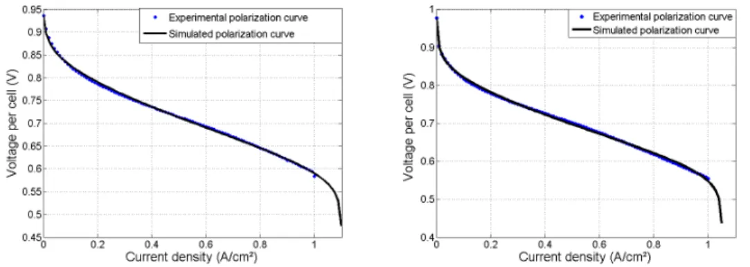
On figure 9 an exemple of the results of this procedure, at the third characterization (after around 182 hours of test) can be seen. The fitting of the polarization curve simulated with the static model is in plain line and the experimental data is in dots for the fuel cell under ripple solicitation. The fitting appears to be satisfying.
Figure 9: Fitting of a polarization curve during the tuning of the static model for the FC2 at the third (182h) and the eight (1016h) characterization
In order to discuss further the accuracy of the model, the results errors MAPE (Mean Absolute percent error) and RMSE (Root Mean Square Error) between the simulated polarization curve and the real data are calculated. As the updating of the static model is realized for each characterization the evolution of the error versus time can be drawn. That allows studying if the model is still adapted when the stack ages. There is no clear evolution with the time (figure 10). It is validated on the experiment under stabilized load as the calculations of error were similar and with no clear tendency. The model is as well adapted at the start of the life of a stack than at its end of life. It is a convenient point, as the goal is to use this model for modeling the ageing.
Figure 10: Evolution of the RMSE and MAPE of the difference between the model and the data with the time for the FC2
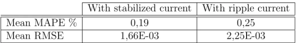
The global errors MAPE and RMSE of the static tuning on the two experiments is then calculated. This value is obtained by taking the average of all the errors obtained on each characterization. The results are gathered on table 2. The good quality of the fitting is one more time validated. The static part of the model reproduces the behavior that can be seen on the experimental data and stay accurate during the 1000 hours of the two tests and for each polarization curve of each test.
With stabilized current With ripple current
Mean MAPE % 0,19 0,25
Mean RMSE 1,66E-03 2,25E-03
Table 2: Mean of errors on all the characterization phases for polarization curve fitting
6.3. Dynamic part tuning validation
During the update of the dynamic part, the fitting with the Nyquist plot is drawn and studied. Figure 11 depicts a Nyquist plot extracted from the experimental data at 35 hours and at 70A for the FC2 and the simulated results obtained thanks to the dynamic model. The mean errors for the two experiments and the simulation of fitting can be found on the table 3. It can be seen that there is one more time no clear evolution of the error with the time or even with the current at which is realized the EIS. This is confirmed as, the same calculation of errors was made on the dynamic part than on the static one, and nor the aging time nor the current has an effect on the performance of the dynamic model.
Figure 11: Fitting of a Nyquist plot at 20 A at the third (182h) and seventh (830h) characterization for the FC2
With stabilized current With ripple current Real part Imaginary part Real part Imaginary part Mean MAPE 0,90 % 8,22 % 0,19 % 0,25 %
Mean RMSE 1,025 12,6 0,0027 0,0026
Table 3: Mean of errors on all the characterization phases for the Nyquist Plot fitting
6.4. Global model simulation
Finally, the global model that can be seen in figure 2 is validated. For that purpose, the model was completely updated with the data from the third characterization (after 182 hours of test) for the FC2. The parameters values obtained thanks to this procedure are gathered in table 4.
The time constant applied to the low pass filter that allows decomposing the current density in a dynamic and a static part is 0.2s.
The global model is then completely updated, it can finally be validated. For that purpose, the load of the experiment is imposed to the model; the simulation and the experiment are then compared.
An example taken after 182 hours around the third characterization can be seen in figure 12. In this figure, it is obvious that the global model responds with the same trend than the fuel cell that was experimented.
Symbol Name Value Unit
r Internal resistance 0.0989 Ω.cm2
En Nernst potential 0.937 V
j0a Exchange current density at the anode 0.1454 A/cm2
ba Tafel anode parameter 36.43 V−1 j0c Exchange current density at the cathode 0.0018 A/cm2
bc Tafel cathode parameter 44.64 V−1 jLc Limit current density at the cathode 1.099 A/cm2 Cdca Double layer capacity at the anode 0.0404 F/cm2 Cdcc Double layer capacity at the cathode 0.0472 F/cm2
L Connector inductance 1.23.10−6 H
j0Oc Parameter of the variation law of ROc 5223 A/cm2 bOc Parameter of the variation law of ROc 0.0012 V−1 kOc Parameter of the variation law of τOc 0.0918 A.s/cm2
Table 4: Values of the parameters after the model updating process with the third char-acterization data around 182h on FC2
However, there is a small difference of a constant value between the two curves when the current is evolving. This can be explained by the change of operating conditions. Indeed, during the polarization curve measurement the operating conditions are different than during the ageing test. For example, the temperature is not stable on this experiment as it exhibits a variation of fifteen degrees. This is due to the poor control of the temperature on the test bench in this specific experiment. So, the hypothesis of of constant operating conditions is not completely verified.
At the open circuit voltage, this difference is bigger and a peak can be observed. It is due to the decomposing block that split the static and the dynamic current. Indeed, this block is a low-pass filter and it is not enough adapted for our needs. Here, the time constant in this block is 0.2s. The influence of this value is interesting. Indeed, if this value is decreased, the peak would rise higher, on an other hand, if this value is augmented, the time the model would take to gain the top of the step, would be too important to face the real behavior of the fuel cell.
The model reproduces well the behavior of the fuel cell as we can see in the figure 12. On this part the error RMSE is 0.5103, a good performance.
7. Conclusion
The objective is to define and validate a model that can accurately re-produce the behavior of a PEMFC in order to be applied for prognostics. For that purpose, in this paper a model composed of a static and a dynamic part is proposed and validated thanks to experimental data. In a first step, the static model is studied by the comparison of experimental polarization curve and simulated one. The errors have been calculated and prove that this part of the model is very satisfying. In a second step, but in the same way, the dynamic part has be examined, the results show a good fitting in-dependently of the time or of the current. Finally, the whole model has been simulated, and it shows good hope for the future application. Indeed, the model is as good on a young stack than on an stack aged of a thousand hours. The model presents the exact same answer to the solicitation that the fuel cell itself under the same solicitation: the behavior is well reproduced. It means that the structure of the model can be kept during the ageing. How-ever, the difference between the operation conditions during the polarization curve and the ageing process is an issue that has to be fixed; the integration of other input might be necessary. The decomposition block would also have
to be improved because it triggers a response not as good as hoped as the decomposition of the current is not well adapted.
This model fits well for the prognostics, and is going to be the starting point of the following work. Indeed, the ageing can be modeled by giving to some parameters a dependency to the time.
Acknowledgment
The research leading to these results has received funding from the Euro-pean Union’s Seventh Framework Programme (FP7/2007-2013) for the Fuel Cells and Hydrogen Joint Technology Initiative under grant agreement num-ber 325275 (SAPPHIRE project). This work has been performed in cooper-ation with the Labex ACTION program (contract ANR-11-LABX-01-01).
References
[1] P. Mootguy, B. Ludwig, N. Steiner, Influence of ageing on the dynamic behaviour and the electrochemical characteristics of a 500 we pemfc stack, International Journal of Hydrogen Energy 39 (19) (2014) 10230 – 10244.
[2] G. Napoli, M. Ferraro, F. Sergi, G. Brunaccini, V. Antonucci, Data driven models for a pem fuel cell stack performance prediction, Interna-tional Journal Of Hydrogen Energy 38 (2013) 11628 – 11638.
[3] C. Robin, M. Gerard, A. A. Franco, P. Schott, Multi-scale coupling between two dynamical models for pemfc aging prediction, International Journal Of Hydrogen Energy 38 (11) (2013) 4675 – 4688.
[4] M.Ceraolo, C. Miulli, A. Pozio, Modelling static and dynamic behaviour of proton exchange membrane fuel cell on the basis of electro-chemical description, Journal of Power Sources 113 (1) (2003) 131 – 144.
[5] K. Goebel, A. Saxena, M. Daigle, J. Celaya, I. Roychoudhury, Introduc-tion to prognostics, in: First European Conference of the Prognostics and Health Management Society, 2012.
[6] R. Gouriveau, K. Medjaher, Chapter 2 : Industrial prognostic - an overview, in: C. B. J. Andrews, L. Jackson (Eds.), Maintenance Mod-elling and Applications, ISBN : 978-82-515-0316-7, Det Norske Veritas (DNV), 2011, pp. 10–30.
[7] M. Lebold, M. Thurston, Open standards for condition-based mainte-nance and prognostic systems, in: 5th Annual Maintemainte-nance and Relia-bility Conference, 2001.
[8] J. Wu, X. Z. Yuan, H. Wang, M. Blanco, J. J. Martin, J. Zhang, Diag-nostic tools in pem fuel cell research : Part i electrochemical techniques, International Journal Of Hydrogen Energy 33 (2008) 1735 – 1746. [9] J. Wu, X. Z. Yuan, H. Wang, M. Blanco, J. J. Martin, J. Zhang,
Diag-nostic tools in pem fuel cell research : Part ii physical/chemical methods, International Journal of Hydrogen Energy 33 (6) (2008) 1747 – 1757. [10] N. Yousfi-Steiner, P. Mootguy, D. Candussoc, D. Hissel, A. Hernandez,
A. Aslanides, A review on pem voltage degradation associated with wa-ter management: Impacts, influent factors and characwa-terization, Journal of Power Sources 183 (2008) 260 – 274.
[11] N. Yousfi-Steiner, P. Mocotguy, D. Candusso, D. Hissel, A review on polymer electrolyte membrane fuel cell catalyst degradation and starva-tion issues: Causes, consequences and diagnostic for mitigastarva-tion, Journal of Power Sources 194 (2009) 130 – 145.
[12] R. Onanena, L. Oukhellou, D. Candusso, A. Same, D. Hissel, P. Aknin, Estimation of fuel cell operating time for predictive maintenance strate-gies, International Journal Of Hydrogen Energy 35 (2010) 8022 – 8029. [13] R. Onanena, L. Oukhellou, D. Candusso, F. Harel, D. Hissel, P. Aknin, Fuel cells static and dynamic characterizations as tools for the estima-tion of their ageing time, Internaestima-tional Journal Of Hydrogen Energy 36 (2011) 1730 – 1739.
[14] C. Cadet, S. Jeme, F. Druart, D. Hissel, Diagnostic tools for pemfcs: from conception to implementation, International Journal of Hydrogen Energy 39 (20) (2014) 10613 – 10626.
[15] R. Petrone, Z. Zheng, D. Hissel, M. Pra, C. Pianese, M. Sorrentino, M. Becherif, N. Yousfi-Steiner, A review on model-based diagnosis methodologies for pemfcs, International Journal of Hydrogen Energy 38 (17) (2013) 7077 – 7091.
[16] Z. Zheng, R. Petrone, M. Pra, D. Hissel, M. Becherif, C. Pianese, N. Y. Steiner, M. Sorrentino, A review on non-model based diagnosis method-ologies for pem fuel cell stacks and systems, International Journal of Hydrogen Energy 38 (21) (2013) 8914 – 8926.
[17] M.Jouin, R. Gouriveau, D.Hissel, M.-C. Pra, N. Zerhouni, Prognostics and health management of pemfc - state of the art and remaining chal-lenges, International Journal Of Hydrogen Energy.
[18] ISO, Condition monitoring and diagnostics of machines, prognostics, Part1: General guidelines, International Standard, ISO13381-1 (2004). [19] R. Gouriveau, Intelligent approaches for phm: overview and challenges,
Aerospace Program Workshop, SIMTech, 2011.
[20] Z.-D. Zhong, X.-J. Zhu, G.-Y. Cao, Modeling a pemfc by a support vector machine, Journal of Power Sources 160 (2006) 293–298.
[21] R. Silva, R. Gouriveau, S. Jeme, D. Hissel, L. Boulon, K. Agbossou, N. Y. Steiner, Proton exchange membrane fuel cell degradation pre-diction based on adaptive neuro-fuzzy inference systems, International Journal of Hydrogen Energy 39 (21) (2014) 11128 – 11144.
[22] S. Morando, S. Jemei, D. Hissel, R. Gouriveau, N. Zerhouni, Predict-ing the remainPredict-ing useful lifetime of a proton exchange membrane fuel cell using an echo state network, in: International Discussion on Hydro-gen Energy and Applications (IDHEA), CNRS - Centre national de la recherche scientifique, 2014, p. 63 (9 pages).
[23] N. Fouquet, C. Doulet, C. Nouillant, G. Dauphin-Tanguy, B. Ould-Bouamama, Model based pem fuel cell state-of-health monitoring via ac impedance measurement, Journal of Power Sources 159 (2) (2006) 905 – 913.
[24] J. hyung Lee, J.-H. Lee, W. Choi, K.-W. Park, H.-Y. Sun, J.-H. Oh, Development of a method to estimate the lifespan of proton exchange membrane fuel cell using electrochemical impedance spectroscopy, Jour-nal of Power Sources 195 (2010) 6001–6007.
[25] U. Reggiani, L. Sandrolini, G. G. Burbui, Modelling a pem fuel cell stack with a nonlinear equivalent circuit, Journal of Power Sources 165 (2007) 224 – 231.
[26] S. Lazarou, E. Pyrgioti, A. T. Alexandridis, A simple electric cir-cuit model for proton exchange membrane fuel cells, Journal of Power Sources 190 (2009) 380 – 386.
[27] N. Siegel, M. Ellis, D. Nelson, M. von Spakovsky, A two-dimensional computational model of a pemfc with liquid water transport, Journal of Power Sources 128 (2) (2004) 173 – 184.
[28] L. Martins, J. Gardolinski, J. Vargas, J. Ordonez, S. Amico, M. Forte, The experimental validation of a simplified pemfc simulation model for design and optimization purposes, Applied Thermal Engineering 29 (2009) 3036–3048.
[29] S. Chevalier, D. Trichet, B. Auvity, J. Olivier, C. Josset, M. Mach-moum, Multiphysics dc and ac models of a pemfc for the detection of degraded cell parameters, International Journal of Hydrogen Energy 38 (26) (2013) 11609 – 11618.
[30] S. Philipps, C. Ziegler, Computationally efficient modeling of the dy-namic behavior of a portable pem fuel cell stack, Journal of Power Sources 180 (2008) 309 – 321.
[31] M. Jouin, R. Gouriveau, D. Hissel, M.-C. Pra, N. Zerhouni, Prognostics of pem fuel cell in a particle filtering framework, International Journal of Hydrogen Energy 39 (1) (2014) 481 – 494.
[32] M. Hinaje, S. Ral, P. Noiying, D. A. Nguyen, B. Davat, An equivalent electrical circuit model of proton exchange membrane fuel cells based on mathematical modelling, Energies 5 (8) (2012) 2724–2744.
[33] S.-K. Park, S.-Y. Choe, Dynamic modeling and analysis of a 20-cell pem fuel cell stack considering temperature and two-phase effects, Journal of Power Sources 179 (2008) 660–672.
[34] A. W. Al-Dabbagh, L. Lu, A. Mazza, Modelling, simulation and con-trol of a proton exchange membrane fuel cell (pemfc) power system, International Journal Of Hydrogen Energy 35 (2009) 5061 – 5069.
[35] Y. Shan, S.-Y. Choe, Modeling and simulation of a pem fuel cell stack considering temperature effects, Journal of Power Sources 158 (1) (2006) 274 – 286.
[36] Y. Hou, Z. Yang, G. Wan, An improved dynamic voltage model of pem fuel cell stack, International Journal Of Hydrogen Energy 35 (20) (2010) 11154 – 11160.
[37] A. Biyikoglu, Review of proton exchange membrane fuel cell models, International Journal Of Hydrogen Energy 30 (2005) 1181 – 1212. [38] E. Laffly, M. Pra, D. Hissel, Pem fuel cell modeling with static-dynamic
decomposition and voltage rebuilding, in: IEEE-ISIE’08, International Symposium on Industrial Electronics, Cambridge, UK, 2008, pp. 1519– 1524.
[39] S. S. Asl, S. Rowshanzamir, M. Eikani, Modelling and simulation of the steady-state and dynamic behaviour of a pem fuel cell, Energy 35 (2009) 1633 – 1646.
![Figure 1: PHM modules adapted from[7]](https://thumb-eu.123doks.com/thumbv2/123doknet/12678412.354224/5.918.308.614.592.900/figure-phm-modules-adapted-from.webp)