HAL Id: hal-01070069
https://hal.inria.fr/hal-01070069
Submitted on 1 Oct 2014
HAL is a multi-disciplinary open access
archive for the deposit and dissemination of
sci-entific research documents, whether they are
pub-lished or not. The documents may come from
L’archive ouverte pluridisciplinaire HAL, est
destinée au dépôt et à la diffusion de documents
scientifiques de niveau recherche, publiés ou non,
émanant des établissements d’enseignement et de
Distributed-Heterogenous Architectures : a Blocking
Approach
Bérenger Bramas, Olivier Coulaud, Guillaume Sylvand
To cite this version:
Bérenger Bramas, Olivier Coulaud, Guillaume Sylvand. Time-Domain BEM for the Wave Equation
on Distributed-Heterogenous Architectures : a Blocking Approach. [Research Report] RR-8604, Inria
Bordeaux Sud-Ouest; INRIA. 2014. �hal-01070069�
0249-6399 ISRN INRIA/RR--8604--FR+ENG
RESEARCH
REPORT
N° 8604
September 2014the Wave Equation on
Distributed-Heterogenous
Architectures : a
Blocking Approach
RESEARCH CENTRE BORDEAUX – SUD-OUEST
Blocking Approach
Bérenger Bramas
∗†, Olivier Coulaud
‡†, Guillaume Sylvand
§Project-Team HiePACS
Research Report n° 8604 — September 2014 — 22 pages
Abstract: The problem of time-domain BEM for the wave equation in acoustics and
electromag-netism can be expressed as a sparse linear system composed of multiple interaction/convolution matrices. It can be solved using sparse matrix-vector products which are inefficient to achieve high Flop-rate whether on CPU or GPU. In this paper we extend the approach proposed in a previ-ous work [1] in which we re-order the computation to get a special matrices structure with one dense vector per row. This new structure is called a slice matrix and is computed with a custom matrix/vector product operator. In this study we present an optimized implementations of this operator on Nvidia GPU based on two blocking strategies. We explain how we can obtain multi-ple block-values from a slice and how these ones can be computed efficiently on GPU. We target heterogeneous nodes composed of CPU and GPU. In order to deal with the different efficiencies of the processing units we use a greedy heuristic that dynamically balances the work among the workers. We demonstrate the performance of our system by studying the quality of the balancing heuristic and the sequential Flop-rate of the blocked implementations. Finally, we validate our implementation with an industrial test case on 8 heterogeneous nodes each composed of 12 CPU and 3 GPU.
Key-words: Parallel Algorithms , Hybrid parallelization , GPU , CUDA , Multi-GPU ,
Time-domain , BEM
∗[email protected] †Inria Bordeaux - Sud-Ouest ‡[email protected]
et hétérogènes : une approche par bloque
Résumé : Dans le domaine temporel, le problème de l’équation des ondes en acoustique et
électromagnétisme peut être définit par un système linéaire creux composé entre autres de matri-ces d’interactions/convolution. Il peut être résolu en utilisant le produit matrice/vecteur creux (SpMV) mais celui-ci n’est pas efficace et atteint une performance très en deçà des capacités des processeurs. Dans ce rapport, nous continuons une approche proposée dans [1] dans laquelle nous changeons l’ordre de calcul afin d’obtenir des matrices ayant un vecteur dense par ligne. Ces ma-trices sont appelées mama-trices tranches et sont calculées à l’aide d’un opérateur matrice/vecteur personnalisé. Ici, nous présentons des implémentations optimisées de cet opérateur sur GPU NVidia reposant sur deux stratégies de blocage. Nous expliquons comment obtenir des blocs de valeurs à partir de matrices tranches et comment les utiliser sur GPU. Nous ciblons les clusters composés de nœuds avec GPU. Afin de prendre en compte les différentes capacités des pro-cesseurs, nous proposons un algorithme glouton qui équilibre le travaille dynamiquement. Nous validons notre système en étudiant la qualité de l’équilibrage et les performances des différentes implémentations. Enfin, nous utilisons notre système sur un cas test industriel en utilisant 8 nœuds chacun étant composé de 12 CPU et 3 GPU.
Mots-clés : Algorithmes Parallèles, Parallélisation Hybride, GPU, CUDA, Multi-GPU,
1
Introduction
Airbus Group Innovations is an entity of Airbus Group devoted to research and development for the usage of Airbus Group divisions (Airbus Civil Aircraft, Airbus Defence & Space, Airbus Helicopters). The numerical analysis team has been working for more than 20 years on inte-gral equations and boundary element methods for wave propagation simulations. The resulting software solutions are used on a daily basis in acoustics for installation effects computation, aeroa-coustic simulations (in a coupled scheme with other tools), and in electromagnetism for antenna siting, electromagnetic compatibility or stealth. Since 2000, these frequency-domain Boundary Element Method (BEM) tools have been extended with a multipole algorithm (called Fast Mul-tipole Method) that allows to solve very large problems, with tens of millions of unknowns, in reasonable time on parallel machines. More recently, H-matrix techniques have enabled the design of fast direct solvers, able to solve problems with millions of unknowns for a very high accuracy without the usual drawback associated with the iterative solvers (no control on the number of iterations, difficulty to find a good preconditioner, etc.). At the same time, we work on the design and on the optimization of the time domain BEM (TD-BEM) that allows to obtain with only one calculation the equivalent results of many frequency-domain computations. In this paper, we focus on the heterogeneous parallel implementation of the algorithm and keep the mathematical formulation described in [3].
In [4], the authors have implemented a TD-BEM application and their formulation is similar to the one we use. They show results up to 48 CPU and rely on sparse matrix-vector product without giving details on the performance. In [5], the author uses either GPU or multi-CPU parallelization and accelerates the TD-BEM by splitting near field and far field. The study shows an improvement of the GPU against the CPU and focuses on the formulation of the near/far computation. The proposed method is a competitive implementation but it is difficult to compare to ours. In [7], they give an overview of an accelerated TD-BEM using Fast Multipole Method. The paper does not contain any information on the sequential performance or even the parallelization which makes it difficult to compare to our work.
The original formulation relies on the Sparse Matrix-Vector product (SpMV) which has been widely studied on CPU and GPU because this is an essential operation in many scientific ap-plications. Our work is not an optimization or an improvement for the general SpMV on GPU because we use a custom operator that matches our needs and which is at the cross of the SpMV and the general matrix-matrix product. Nevertheless, the optimizations of our implementation on GPU have been inspired by the recent works which include efficient data structures, memory access pattern, global/shared/local memory usage and auto-tunning, see [8] [9] [10] [11]. These studies show that the SpMV on GPU has a very low performance against the hardware capacity and motivate the use of blocking which is crucial in order to improve the performance. The method to compute multiple small matrix/matrix products from [12] has many similarities with our implementation (such as the use of templates for example). In this paper we do not com-pare our CPU and GPU implementations rather we focus on the GPU and propose a system to dynamically balance the work among workers.
This paper addresses two major problems of the TD-BEM solver. Firstly, we propose an efficient computation kernel for our custom multi-vectors/vector product on GPU. Secondly, we propose novel parallelization strategies for shared heterogeneous distributed memory platforms. The rest of the paper is organized as follows. Section 2 provides the background and the mathematical formulation of the problem and describes the usual algorithm. Then we introduce the slice matrix structure and the multi-vectors/vector product in Section 3. Section 4 describes the blocking schemes and the GPU implementations. Section 5 details the parallelization strate-gies and the balancing algorithm. Finally, in Section 6 we provide an experimental performance
evaluation of our multi-vectors/vector operator on GPU and CPU and illustrate the parallel behavior with an industrial test case.
2
Time-Domain BEM for the Wave Equation
2.1
Formulation
Our formulation has been originally introduced in [3] but in order to keep this paper self-explanatory, we present the relevant aspects of the TD-BEM. An incident wave w with a velocity
c and a wavelength λ is emitted on a boundary Ω. This surface Ω is discretized by a classical
finite element method which leads to N unknowns. The wave equation is also discretized in time with a step ∆t and a finite number of iterations driven by the frequency interval being study. In fact, increasing the number of time steps improves the results towards the bottom of the
frequency range considered. At iteration time tn= n∆t, the vector ln contains the illumination
of w over the unknowns from one or several emitters. The wave illuminates the location where the unknowns are defined and is reflected by these ones over the mesh. It takes a certain amount of time for the waves from the emitter or an unknown to illuminate some others. This relation
is characterized by the interaction/convolution matrices Mk.
Using the convolution matrices Mk, and the incident wave ln emitted by a source on the
mesh, the objective is to compute the state of the unknowns an at time n for a given number of
time iterations. The problem to solve at time step n is defined by
Kmax
X
k≥0
Mk· an−k= ln. (1)
The original equation (1) can be rewritten as in formula (2) where the left hand side is the state to compute and the right hand side is known from the previous time steps and the test case definition. an = (M0)−1 ln− KXmax k=1 Mk· an−k ! . (2)
2.2
Interaction/Convolution Matrices
The matrix Mk contains the interactions between unknowns that are separated by a distance
around k.c.∆t and contains zero for unknowns that are closer or further than this distance. These N × N matrices are positive definite and sparse in realistic configuration. They have the following properties:
• The number of non-zero values for a given matrix Mkdepends on the structure of the mesh
(the distance between the unknowns) and the physical properties of the system c, λ and ∆t.
• For k > Kmax= 2+ℓmax/(c∆t), with ℓmax= max(x,y)∈Ω×Ω(|x−y|)the maximum distance
between two unknowns, the matrices Mk are null.
The construction of these matrices is illustrated in Figure 1. The matrices are filled with values depending on the delay taken by a wave emitted by an unknown to pass over another one.
The position of the non-zero values in the matrices is driven by the numbering of the
A B C A B C A B C (a) M0 A B C A B C A B C (b) M1 A B C A B C A B C (c) M2 A B C A B C A B C (d) M3
Figure 1: Example of Mk matrices for three unknowns A, B, C in 1D. A wave emitted from
each unknown is represented at every time steps. When a wave is around an unknown, a value
is added in the matrix which is symbolized by a gray square. All matrices Mk with k > 3 are
zero since the highest distance between elements is ≤ 3.c.∆t.
unknowns j and j + 1 are both at a distance k.c.∆t from i. On the other hand, two NNZ values
are contiguous on a column, for example Mk(i, j) and Mk(i + 1, j) if the unknowns i and i + 1
are both at a distance k.c.∆t from j. Therefore, numbering consecutively the unknowns that are spatially close is a way among others to increase the chance to have contiguous values in the interaction matrices.
2.3
Resolution Algorithm
The solution is computed in two steps. In the first step, the past is taken into account using the
previous values of ap with p < n and the interaction matrices as shown in Equation (3). The
result sn is subtracted from the illumination vector, see Equation (4).
sn = KXmax k=1 Mk· an−k, (3) e sn = ln− sn. (4)
In the second step, the state of the system at time step n is obtained after solving the following linear system
M0an
= esn. (5)
The first step is the most expensive part, from a computational standpoint. The solution of
Equation (5) is extremely fast, since the matrix M0 is symmetric, positive definite, sparse and
almost diagonal. We can solve it by using a sparse direct solver for example.
Context of the application Our application is a layer of an industrial computational
work-flow. We concentrate our work on the solution algorithm and we delegate to some black-boxes
the generation of the values of the interaction matrices and the factorization of M0. Moreover,
in our simulations the mesh is static and all the interaction matrices and the pre-computation needed by the direct solver are performed once at the beginning. The most costly part of our
3
Re-ordering the Summation Computation
3.1
Ordering Possibilities
We refer to the process of computing sn as the summation stage. This operation uses the
interaction matrices Mk and the past values of the unknowns an−k (with k strictly positive).
A natural implementation of this computation is to perform Kmax independent SpMV. That is
implemented with four nested loops. The first loop is over the time step denoted by index n. The second loop is over the interaction matrices and is controlled by index k in our formulation
and goes from 1 to Kmax. Finally, the two remaining loops are over the rows and the columns
of the matrices and are indexed by i and j respectively. The indices i and j cover the unknowns and go from 1 to N. The complete equation is written in Equation (6) where all indexes n, k, i and j are visible.
sn(i) = kmax X k=1 N X j=1 Mk(i,j) × an−k(j) , 1 ≤i≤ N . (6)
In term of algorithm, there is no need to keep the outer loop on index k and two other orders of summation are possible using i or j. The three possibilities are represented in Figure 2 where
all interaction matrices Mk are shown one behind the other and represented as a 3D block.
This figure illustrates the three different ways to access the interaction matrices according to the outer loop index. The natural approach using k is called by front and usually relies on SpMV (Figure 2a). From [1], we propose to use a different approach called by slice using j as outer loop index. The data access pattern of the interaction matrices in slice is illustrated in Figure 2c.
A0 M6 A1 M5 A2 M4 A3 M3 A4 M2 A5 M1 S6 (a) Front (k) A0 M6 A1 M5 A2 M4 A3 M3 A4 M2 A5 M1 S6 (b) Top (i) A0 M6 A1 M5 A2 M4 A3 M3 A4 M2 A5 M1 S6 (c) Slice (j)
Figure 2: Three ways to reorder the computation of sn with current time step n = 6, number of
unknowns N = 8 and Kmax = 6. (a) The outer loop is on the different Mk matrices. (b) The
outer loop is over the row index of Mk and sn. (c) The outer loop is over the column index of
3.2
Slice Properties
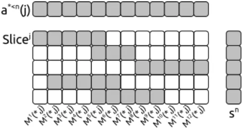
We denote by slice the data when the outer loop index of the summation is j in Equation 6. The
concatenation of each column j of the interaction matrices [M1(∗, j) M2(∗, j) ... MKmax(∗, j)]
is called Slicej as illustrated in Figure 2c. This definition induced the relation Mk(i, j) =
Slicej(i, k). Therefore, a slice is a sparse matrix of dimension (N × (K
max− 1)). It has a
non-zero value at line i and column k if d(i, j) ≈ k · c · ∆t, where d(i, j) is the distance between the
unknowns i and j. From the formulation, an interaction matrix Mk represents the interaction
between the unknowns for a given time/distance k. Whereas a Slicej represents the interaction
that one unknown j has with all others over the time. This provides an important property to the sparse structure of a slice: the non-zero values are contiguous on each line. In fact, it takes several iterations for the wave emitted by an unknown to cross over the other. In other
words, for a given row i and column j all the interaction matrices Mk that have a non zero value
at this position are consecutive in index k. In the slice format, it means that each slice has one vector of NNZ per line but each of this vector may start at a different column k. If it takes p time
steps for the wave from j to cross over i, then Slicej(i, k) = Mk(i, j) 6= 0, k
s≤ k ≤ ks+ pwhere
ks = d(i, j)/(c∆t). We refer to these dense vectors on each row of a slice as the row-vectors.
Using the interaction matrices, we multiply a matrix Mk by the values of the unknown at time
n − k (an−k(∗)) to obtain sn. When we work with slices, we multiply each slice Slicej by the
past value of the unknown j (a∗<n(j)). An example of slice is presented in Figure 3.
a*<n(j) M1(* ,j) Slicej sn M2(* ,j) M3(* ,j) M4(* ,j) M5(* ,j) M6(* ,j) M7(* ,j) M8(* ,j) M9(* ,j) M10 (*,j) M11 (*,j) M12 (*,j)
Figure 3: An example of Slice where the non-zero values are symbolized by gray squares and
zero by white squares. The vector a∗<n(j)contains the past values of the unknown j. The vector
sn will contain the current result of the summation stage for t = n.
When computing the summation vector snwe can perform one scalar product per row-vector.
Then, sn can be obtained with N × N scalar products (there are N slices and N rows per slice)
instead of Kmax SpMV.
3.3
Slice Computational Algorithm with Multiple Steps
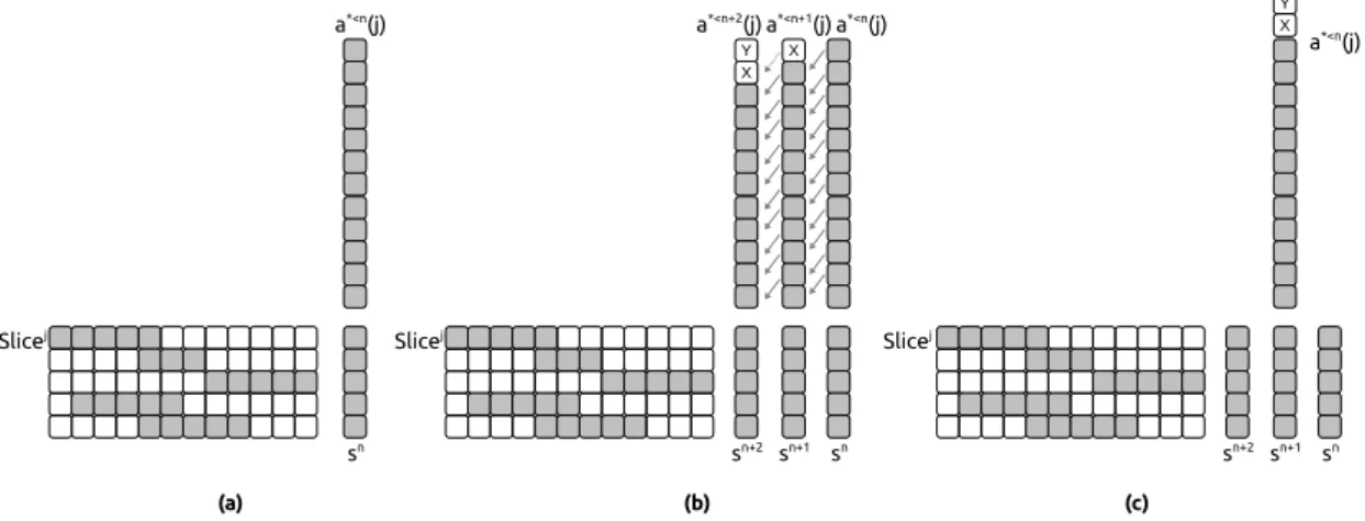
The scalar product, which is a level 1 BLAS, has a low ratio of floating point operations (Flop) against loaded data. In fact, one needs to load one value from both vectors in order to perform one multiplication and one addition. More precisely, by calling d the dimension of the vector, we need to load 2d + 1 values to perform 2d Flops. Figure 4a shows how we compute a slice using one scalar product per row. In [1] we propose two optimizations to increase this ratio.
The first optimization is to work with several summation vectors at a time. At time step n,
we try out to compute the current time step summation vector sn and the next step summation
vector sn+1 together. When computing a summation vector we use the slice matrices which
remain constant and the past values of the unknowns relatively to a given time step. The vector
sn requires the past values ap<n whereas we need the past values ap<n+1to compute the vector
yet. If we replace an by zero we are able to compute sn and a part of sn+1 together. Therefore,
we perform a matrix-vector product instead of a scalar product. The vectors are the non-zero row-vectors of the slices and the matrices are the past values which match the summation vectors
sas illustrated by Figure 4b. We called ngthe number of summation vectors that are computed
together. Once the summation is done, if ng = 2 we end up with sn and sn+1. Because we
replaced an with zero, sn+1 is not complete. We continue the usual algorithm with sn and
obtain an after the resolution step (Equation 5). Then, this result an is projected to sn+1 using
SpMV and M1and let us obtain the complete summation vector sn+1. We refer to this projection
as the radiation stage. It is possible to have ng greater than 2 but the higher is ng the more
important the radiation stage becomes. In this configuration, we load d + ng+ d × ng to perform
ng× 2dFlops.
The second optimization takes into account the properties of the past values. When working
with the Slicej, we need the past values of the unknown j: sn needs ap<n(j) and sn+1 needs
ap<n+1(j). The vector ap<n+1(j)is equal to the vector ap<n(j)where each value is shifted by one
position and with an(j)as first value (or zero if this value does not exist at that time). In order
to increase the data reuse and to have less loading we consider only one past values vector for the
ng summation vectors involved in the process. We take the existing values ap<n(j)and append
one zero for each ng> 1 as it is shown in Figure 4c. In this case, we load d + ng+ (d + ng− 1)
to perform ng× 2dFlops. This operator is called multi-vectors/vector product and is detailed
in Figure 5. a*<n(j) Slicej sn a*<n+1(j) Slicej sn+1 X a*<n(j) sn a*<n+2(j) sn+2 Y X Slicej sn+1 a*<n(j) sn sn+2 Y X (a) (b) (c)
Figure 4: Summation stage with Slicejand 3 possibilities. (a) With n
g= 1using scalar product.
(b) With ng= 3using matrix/vector product (X and Y are the values of a not yet available and
replaced by zero). (c) With ng = 3using the multi-vectors/vector product.
4
Slice Computation on GPU
In [1] we propose an efficient way to compute the multi-vectors/vector products on CPU us-ing SIMD (SSE or AVX). This method is no longer efficient for GPU because of its hardware particularities that we resume briefly before introducing two methods to compute a slice on this device. One can see a GPU as a many-threads device or a large SIMD processor unit. It executes several team of threads (also called group or wrap). Different levels of memory exist in most of the GPU. The global memory can be accessed and shared by all the threads but is slow and is
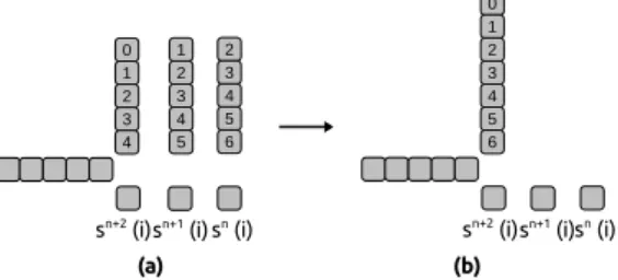
sn+2 (i)sn+1 (i) sn (i) 0 1 2 3 4 0
sn+2 (i)sn+1 (i)sn (i) 1 2 3 4 5 6 1 2 3 4 5 2 3 4 5 6 (a) (b)
Figure 5: Computing one slice-row with 3 vectors (ng= 3): (a) using 3 scalar products and (b)
using the multi-vectors/vector product.
slowed down if the access is unaligned/uncoalesced inside a thread team. The shared memory is fast and shared among the threads of the same team but is very limited in size. Finally, each thread has dedicated registers/local memory. Therefore our original approach from [1] is not
efficient on GPU because it will need extensive reductions/merges or very large ng (equal to the
number of threads in a team for example).
That is why we work with block of data instead of vectors. We present two cut-out strategies that split a slice into multiple pieces of the same size, the Full-Blocking and the
Contiguous-Blocking approaches. We call these pieces blocks and their dimension br (the number of rows)
and bc (the number of columns). In both cases bc should be at least equal to dmaxwhich is the
longest row-vector in all the slices of the simulation. Moreover, we add a constraint that each row-vector must belong fully to only one block and cannot be subdivided. These are important criteria to implement efficient GPU kernels and cut-out algorithms. We have compared this
approach to a dynamic block height br by increasing the blocks until a row-vector is out or
even by using a dynamic programming approach to have the fewest blocks as possible. But the extra-costs of seeking the best block configuration or having unpredictable block sizes are too significant.
4.1
Full-Blocking Approach
In this approach we extract and copy parts of the slices into blocks and let the original structure of the values unchanged. A block contains the row-vectors that are inside a 2D interval of
dimension br per bc. If two row-vectors are separated by more than br rows or if they have
some values separated by more than bc columns, they cannot be in the same block. Several
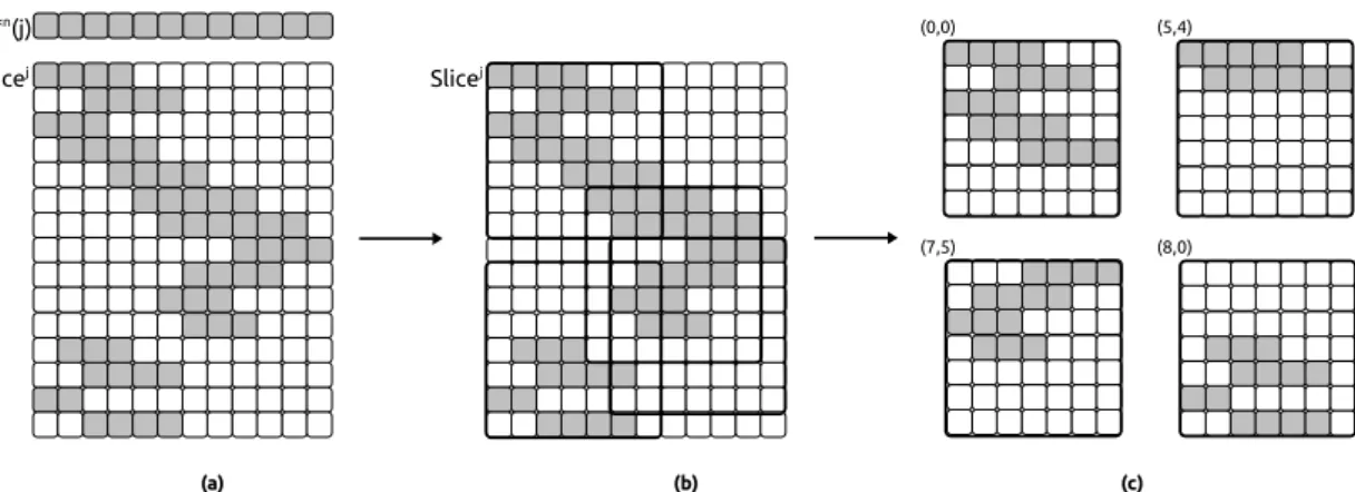
algorithms exist in order to cut-out a slice matrix into blocks. Our implementation is a greedy heuristic which has a linear complexity with respect to the number of rows in the slices. The algorithm starts by creating a block at the first row (for the first row-vector). Then it progresses row by row and starts a new block whenever the current row-vector does not fit in the current block. Figure 6 shows an example of cut-out using this algorithm and the resulting blocks. The generated blocks remain sparse in most cases. The algorithm assigns a pair of integers to each block which corresponds to the position of the upper-left corner of these ones in the original slices as shown in Figure 6c.
Using blocks the computation we have to perform is identical to the multi-vectors/vector product introduced in Section 3.3 and is called the multi-vectors/matrix product. It is also similar to a matrix/matrix product with a leading dimension of one in the past values (which is not a matrix but a special vector).
In this paragraph and in Figure 9 we describe the implementation details of this operator on
Slicej a*<n(j) Slicej (0,0) (5,4) (7,5) (8,0) (a) (b) (c)
Figure 6: Example of a slice cut-out into blocks with the Full-blocking approach : (a) the original slice, (b) the blocks found by the greedy algorithm and (c) the blocks as they are going to be
computed with their corner positions in the original slice. The block dimension is bc= 7 × br= 7.
threads copy the past values needed by a block in a shared memory array of size bc+ ng− 1.
Each thread treats one row of the block and computes ng results. The outer loop iterates bc
times over the columns of the block. The inner loop iterates ngtimes to let the threads compute
the result by loading a past value and using the block values. The ng results are stored into
local/register variables which are written back to the main memory once a thread has computed its entire row. In this approach the threads read the block values from the global memory once
and in an aligned fashion column per column. Also, ng and bc are known at compile time, thus
the loops over the columns and the results are unrolled.
Slicej Kmax-1 N a*<n(j) I) Copy to shared memory III) Add to global memory
II) Aligned access in global memory
III) Partial results in registers
sn
sn+1
sn+2
II) Read from shared memory
Global Memory Shared Memory Local Memory
(a) (b) (c) b c b r Thread-1 Thread-2 Thread-3 Thread-4 Thread-5 Thread-6 Thread-7 Thread-8 Thread-9
Figure 7: Example of the computation of a block from Full-blocking on GPU with ng = 3,
bc= 16and br= 9: (a) the original slice is split in block during the pre-computation stage, (b)
the blocks are moved to the device memory for the summation stage and (c) a group of threads is in charge of several blocks and compute several summation vectors at the same time by doing a multi-vectors/matrix product. In c − I) the threads copy the associate past values, in c − II) each thread computes a row and in c − III) threads add the results to the main memory.
The drawback of this method is the number of generated blocks and thus the extra-zeros
padding. In the worse case this method can generate one block of dimension br× bc per row.
Such configuration occurs if br is equal to one or if each row-vector starts at a very different
column compare to its neighbors. So bc should be large enough to reduce the number of blocks
but the larger bc is the more zeros are used to pad. The numbering of the unknowns is also
an important criteria because the positions of the NNZ values depend on it. However the main advantage of this method is that all rows in a block depend on the same past values.
4.2
Contiguous-Blocking Approach
In this approach, instead of extracting blocks as they are originally in the slices, we copy each row separately in the blocks. Therefore, two row-vectors can be in the same block if they are
separated by less than br lines no matter the positions of their values in the columns. In the
Full-Blocking, all rows from a block have been copied from the same columns in the original slice. On the contrary, in the Contiguous-Blocking this is not guaranteed and each row of a block may come from different columns of the slices as shown by Figure 8. That is why we need to store the origin of the rows in the slices in a vector to be able to compute them with the correct past values, see Figure 8c.
Slicej a*<n(j) Slicej (0) (+) (14) 0 2 0 1 3 4 5 8 6 5 6 1 2 0 2 0 0 0 0 0 0 (a) (b) (c)
Figure 8: Example of a slice cutting-out into blocks with the Contiguous-Blocking approach : (a) the original slice, (b) the block build one row after the other and (c) the blocks as they are stored and computed with the starting point of each row in the original slice. The block dimension is
bc= 7 × br= 7.
The kernel implementation of the Contiguous-Blocking is very similar to the Full-Blocking except that it must take into account the column differences. Instead of copying the past values needed for a block in the shared memory, the threads copy all the past values needed for a slice and thus for the blocks coming from the same slice. Then the threads of a team no longer access the same past values but each thread accesses the past values that match the starting point of the row it has to compute. The threads continue to read the block values as they do in the Full-Blocking with a regular pattern.
The Contiguous-Blocking always generates round up(N/br)blocks per slice. The number of
columns in a block bc must be at least equal to the longest row-vector dmax but there is no
advantage to have bc greater than dmax. Knowing the block size and the number of unknowns,
we know the total number of values in the system generated by the Contiguous-Blocking: N ×
Slicej
Kmax-1
N
a*<n(j)
I) Copy once the vector to shared memory
III) Add to global memory
II) Aligned access in global memory
III) Partial results in registers
snsn+1sn+2
II) Unaligned read from shared memory
Global Memory Shared Memory Local Memory
(a) (b) (c) b c b r Thread-1 Thread-2 Thread-3 Thread-4 Thread-5 Thread-6 Thread-7 Thread-8 Thread-9
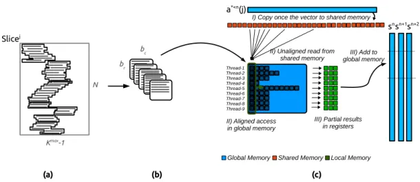
Figure 9: Example of the computation of a block from Contiguous-Blocking on GPU with ng= 3,
bc = 11 and br = 9 : (a) the original slice is split in block during the pre-computation stage,
(b) the blocks are moved to the device memory for the summation stage (c) A group of threads is in charge of all blocks from a slice interval and compute several summation vectors at the same time by doing a multi-vectors/matrix product. In c − I) the threads copy the past values associated to a slice, in c − II) each thread computes a row and read the past values that match it own row and in c − III) threads add the results to the main memory.
there are N × N × dav NNZ values and the blocks are padded with bc− dav zeros per row in
average.
5
Parallel Heterogeneous Algorithm
5.1
Distributed Memory Algorithm
Parallelization We consider the parallelization approach proposed in [1] for CPU where each
node has an interval of the slices and computes an amount of the summation sn. Then all nodes
are involved in the factorization/resolution and compute the current time step an.
Communica-tions between nodes only occur during the resoluCommunica-tions and depend on the external solver.
Inter-nodes balancing In our configuration, we consider that the nodes are similar and have
the same computational capacity. We try to make each node having an interval of the slices that contains the same amount of data in order to balance the summation work. Since the resolution is a critical operation that involves all the nodes, balancing the summation work between nodes is crucial for the application to reduce the synchronization time between iterations.
5.2
Shared Memory Algorithm
Parallelization A worker defines a processing unit or a group of processing units on the same
node. We dedicate one core to manage one GPU and to be in charge of the kernel calls and the data transfers. A GPU-worker is a couple of CPU/GPU. All the cores from a node that are not in charge of a GPU are seen as a single entity called CPU-worker. So one node is composed of one
GPU-worker per GPU and one single CPU-worker as shown in Figure 10. All the workers take part in the summation step but only the CPU are involved during the resolutions/factorization. Inside a CPU-worker we balance the work between threads as we do with nodes by assigning to each thread the same amount of data.
CPU GPU CPU GPU CPU GPU CPU CPU CPU CPU CPU CPU CPU CPU CPU (a) (b)
Figure 10: Example of workers on a node composed of 12 CPU and 3 GPU : (a) the CPU worker composed of all the CPU that are not in charge of a GPU, (b) three GPU workers each composed of a couple of CPU/GPU.
Dynamic balancing between workers A node wi is in charge of an interval of the slices
[Ai; Bi]and computes a part of the summation sn. But this interval has to be balanced between
the different workers within the node. We constrain each worker to have a contiguous interval of data. Also, workers can have different computational capacities and the slices can have different costs. Therefore, the problem is to find the optimal interval for each worker that cover the node slices and with the minimum wall time. The walltime is the maximum time taken by a worker to compute its interval.
One possibility to solve this problem is to perform a calibration/tunning and to estimate the speed of each worker. But such approach takes a non negligible time and it is difficult to consider all the possible configurations and the data transfers. We could also perform a warm-up stage and have each worker computes the full slice interval to know the computation time taken for each worker for each slice. Not only this process can be extremely slow but the fastest worker for each slice individually may not be the fastest to compute a given interval. In fact, the GPU are much more limited by their memory than the CPU and if we assign a slice interval to a GPU that does not fit in its memory it will induce very slow copy (from CPU to GPU or even from hard-drive to GPU). We propose to balance the work after each iteration in order to improve the next ones. Plenty of heuristics are possible to perform such operation and we propose a greedy algorithm with a O(W ) complexity, where W is the number of workers.
The algorithm we propose considers that the average time ta of all workers in the previous
iteration is the ideal time and the objective for the next iteration. For the first iteration we
assign the same number of slices to each worker. At the end of the iteration, each worker wi has
computed its complete interval of slices [ai; bi]in time ti. We do not measure the time taken for
each individual slice but we have an estimation of the cost ci = ti/si, with si = bi− ai+ 1the
number of elements computed by the worker of index i.
Workers that were slower than average (if ta < ti) should reduce their intervals. Whereas, the
faster workers (if ti < ta) should increase their intervals and compute more slices. We consider
that each slice on a given worker has the same cost. Therefore, for a slow worker wi we remove
ri = (ti− ta)/ci slices from its interval. We would like to do the same for a faster worker and
add oi= (ta− ti)/ci to its intervals. But in most cases the number of elements to remove from
the slower workers is not equal to the number of elements we want to give to the faster workers. For example, in a system with two workers and the following properties in the previous iteration
elements in t2 = 4s. The average execution time is ta = (10 + 6)/2 = 8sand the first worker
should remove r1 = (10 − 8)/(10/10) = 2/1 = 1 element whereas the second worker should
increase its interval with o2= (8 − 4)/(4/3) = 4/(4/3) = 3 elements.
So the faster workers have to share the slices that have been removed. We sum the number
of available slices Sremoved=Pri as the number of required slices Sgiven=Poi and distribute
using a weight coefficient. A faster worker will have its interval increased by oi∗ Sremoved/Sgiven
which guarantee an equality between the slices removed and given. The number of slices to
compute is updated for each worker (si = si− ri or si= si+ oi∗ Sremoved/Sgiven) and then a
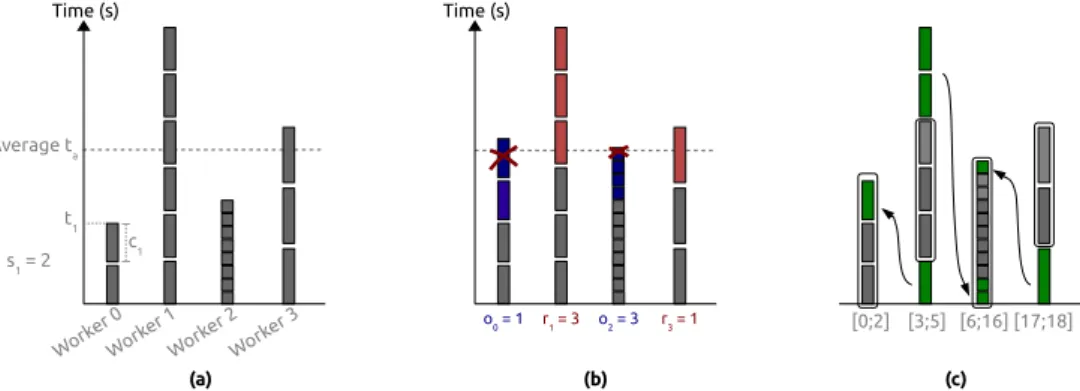
new contiguous slice interval is assigned to each worker. An example of this heuristic is presented in Figure 11. Time (s) Average ta Time (s) r1 = 3 o2 = 3 r3 = 1 o0 = 1 (a) (b) (c) Worke r 0 Worke r 1 Worke r 2 Worke r 3 t1 c1 s1 = 2 [0;2] [3;5] [6;16] [17;18]
Figure 11: Illustration of one iteration of the balancing algorithm with 4 workers. Workers 1 and
3are above the average and should drop 3 blocks and 1 block respectively (red blocks). Workers
0and 2 are under the average and should acquire 1/4 and 3/4 of the dropped blocks respectively
(blue blocks).
This algorithm should find an optimal solution in one iteration if there is the same amount of work per element. But there is no warranty that the algorithm can find the optimal solution or even that it improves as it iterates. Theoretically, we can stop the algorithm if a configuration does not give a better result than the previous one. But in practice some latency or unpredictable events make this statement unsafe. This is why in practice we stop the algorithm after a given number of iterations and rollback to the best configuration that was generated.
6
Performance and Numerical Study
6.1
Experimental Setup
Hardware configuration We use up to 8 nodes and each node has the following configuration:
2 Hexa-core Westmere Intel® Xeon® X5650 at 2.67GHz and 36GB (DDR3) of shared
memory and 3 NVIDIA Tesla M2070 GPU (1.15GHz), 448 Cores, 6GB (GDDR5) of dedicated memory. Peak performances are 10.68 GF lops/s in double and 21.36 GF lops/s in single for one CPU core and 515 GF lops/s in double and 21.36 GF lops/s 1.03 T F lops/s in single for one GPU. The nodes are connected by an Infiniband QDR 40 Gb/s network.
Compiler and libraries We use the Gcc 4.7.2 compiler and Open-MPI 1.6.5. The compilation
flags are -m64 -march=native -O3 -msse3 -mfpmath=sse. The direct solver is a state of the art solver Mumps 4.10.0 [17] which relies on Parmetis 3.2.0 and Scotch 5.1.12b. The calculations are
performed in Single (32 bit arithmetic) or Double (64 bit arithmetic). Parallelization over nodes is supported by MPI [18] and parallelization inside nodes over shared memory by OpenMP [19].
6.2
Balancing Quality
In Section 5.2 we described the heuristic we use to balance the summation work among workers inside a node. We now test this method empirically in order to know how far from the optimal choice it is. We test different configurations by changing the amount of work per element or the acceleration factor of the workers as shown in Table 1.
❤❤ ❤❤ ❤❤ ❤❤ ❤❤ ❤❤ ❤❤❤ Work distribution Worker heterogeneity Up-Down 0.0% 0.1% 0.1% 0.0% Up-Up 0.0% 0.0% 0.1% 0.1% Up 0.1% 0.1% 0.2% 0.2% Random 0.0% 0.0% 0.2% 0.0% Stable 0.0% 0.0% 0.1% 0.1%
Table 1: Balancing Algorithm Vs. Optimal Choice. Extra-cost of the dynamic balancing
algorithm against the optimal choice after 40 iterations with 6 workers and 10, 000 elements. A zero score means that the optimal choice has been achieved.
For each test we generate two arrays, one for the costs using different distributions and the second for the acceleration factors for the workers. We get a worker virtual execution time by multiplying the sum of the costs from its interval and its acceleration factor. The configuration virtual wall time is obtained by taking the maximum virtual execution time of all workers. The balancing algorithm is executed during a given number of iterations and compared to the optimal choice. We find the optimal balance using dynamic programming, that is finding the contiguous interval for each worker that has the minimum wall time. Table 1 shows that the balancing algorithm is close to the optimal even when the cost per element or the worker acceleration factors are very heterogeneous.
6.3
Sequential Flop-rate
6.3.1 Full-Blocking Kernel Flop-rate
Table 2 presents the Flop-rate of the GPU and the CPU implementations for the blocks generated by the Full-Blocking method described in Section 4.1. We look at the Flop-rate achieved by one
GPU or one CPU core for different sizes of dense block. On the GPU we create 128 teams of br
threads each. As expected the performance increases with the block size. On GPU increasing
brincreases the number of threads and increasing bcgive more work to each thread individually
and let unroll larger loops. The CPU implementation benefits also of the instruction pipelining
when we increase br and do not have special improvement when we increase bc. We remind
that increasing the size of the blocks should reduce the number of generated blocks but it also increases the zero padding. So finding the correct dimension is a matter of finding the fastest kernel for the generated number of blocks.
GPU CPU ❤❤ ❤❤ ❤❤ ❤❤ ❤❤ Height (br ) Width (bc ) 16 32 64 128 16 32 64 128 Single 16 37 54 70 78 2.7 2.7 2.8 2.8 32 56 91 130 168 4.2 8.2 8.3 8.3 64 70 114 169 222 8.4 8.5 8.5 8.5 128 86 137 194 245 7.8 7.9 7.9 8 Double 16 27 38 48 57 2.6 2.6 2.6 2.7 32 35 54 75 93 4.2 4.2 4.3 4.3 64 43 64 90 114 3.8 3.8 3.9 3.9 128 51 77 104 125 3.8 3.8 3.8 3.9
Table 2: Performance of computing the blocks from Full-Blocking. Performance in GF lops/s
taken from the computation of 256 slices composed of 6400 rows and bc columns and with 128
GPU thread teams.
6.3.2 Contiguous-Blocking Kernel Flop-rate
Table 3 presents the Flop-rate of the GPU and CPU implementations for the blocks generated by the Contiguous-Blocking method described in Section 4.2. The GPU implementation has the same behavior as the Full-Blocking implementation as we increase the block sizes but succeed to go a little faster. So the GPU Contiguous-Blocking is not paying extra-cost of irregular shared memory accesses. Moreover, this implementation copies all the past values needed by the block of the same slice in the shared memory which seems to be an advantage compare to the GPU Full-Blocking which copies past values for each block (smaller copies but more frequently). In the other hand, the CPU implementation is having a extra-cost because of the irregular past values access compare to the CPU Full-Blocking which divide the performance by four. We
remind that for a given simulation, the Contiguous-Blocking have a bc equal to dmax and thus
there is no choice in the block width. Whereas we can choose br which reduce the number of
block generated from a slice and increase the number of GPU threads per team. For example,
if the longest row-vector of a simulation dmax is equal to 16 we will chose br equal to 128 in
single precision. The source code of the Contiguous-Blocking kernel implementation is given in Appendix ??. GPU CPU ❤❤ ❤❤ ❤❤ ❤❤ ❤❤ Height (br ) Width (bc ) 16 32 64 128 16 32 64 128 Single 16 39.0 57.1 73.6 85.3 2.2 2.3 2.1 2.1 32 57.8 85.2 112.8 134.0 4.1 4.7 4.1 3.8 64 84.3 126.8 165.8 201.0 4.7 4.8 4.1 2.9 128 106.5 162.6 220.0 267.0 4.6 4.4 2.6 2.5 256 103.0 156.6 211.6 257.4 4.0 2.4 2.1 2.0 Double 16 25.5 35.6 44.2 50.4 2.6 1.7 1.7 1.6 32 39.4 56.3 71.9 83.7 2.6 2.2 2.0 1.6 64 50.4 74.3 98.9 117.2 2.4 2.0 1.5 1.5 128 55.5 83.1 110.1 131.7 2.2 1.5 1.4 1.3 256 58.6 88.5 118.9 143.0 1.4 1.4 1.3 1.2
Table 3: Performance of computing the blocks from Contiguous-Blocking. Performance in
GF lops/staken from the computation of 256 slices composed of 6400 rows and bc columns and
with 128 GPU thread teams.
6.4
Test Case
We now consider a real simulation to study the parallel behavior of the application. Our test case is an airplane composed of 23 962 unknowns shown in Figure 12. The simulation should perform
10 823time iterations. There are 341 interaction matrices. The total number of non-zero values
in the interaction matrices, except M0, is 5.5 × 10⁹. The longest row-vector d
max is 15 and the
the summation sn is around 11 GF lops/s. If we consider that the resolution of the M0 system
has the cost of a matrix-vector product, the total amount of Flops for the entire simulation is 130 651 GF lop/s. We compute the test case in single precision. In this format we need 50 GB to store all the data of the simulation. Our application can execute out-of-core simulations, but we concentrate our study on in-core executions. We need at least 2 nodes to have the entire test case fitting in memory.
Figure 12: Illustration of the Airplane test case
6.4.1 Number of Blocks from the Full-Blocking
The Full-Blocking generates blocks from a given slice depending on the block size (br and bc)
and the position of the NNZ values inside the slice. Therefore, the numbering of the unknowns if crucial to decrease the number of generated blocks. We have tested different ordering methods but the spatial ordering gave the better results (the comparison is not given in the current study). For example we have tried to number the unknown by solving a Traveling Salesman Problem using one or several interaction matrices as proposed in [16]. Here we present the results for the Morton indexing [14] and the Hilbert indexing [15]. In both cases we compute a unique index for each unknown and sort them according it. It is possible to score the quality of the ordering by
looking at the contiguous values between the row-vectors. If two consecutive row-vectors vj
i and
vi+1j from Slicej have q
j
i,i+1 values on the same columns, we describe the quality between these
two rows as (qj
i,i+1)2. The quality of a slice is the average quality between its rows and the quality
of the entire system is the average quality of the slices. Using the original ordering provided by the mesh generation the ordering score for all the slices is 33. By ordering the unknowns using Morton and Hilbert index we obtain the scores 54 and 55 respectively. This means that using these spatial ordering the quality increase and most of the consecutive row-vectors have values on the same columns.
Table 4 shows the number of blocks depending on the type of ordering and the size of the blocks when we process the slices of the test case using the Full-Blocking from Section 4.1. It is clear that numbering of the unknowns with a space filling curve reduces drastically the number of blocks (NBB in the table). The table also contains an estimation of the computation time E≈ to process the generated blocks with one GPU using the performance measures from Table 2. We can see that increasing the size of the blocks does not always reduce the number of blocks.
For example, with the Morton Indexing and any bc, we have the same number of blocks for br
equals to 32 or br equals to 64.
These results show the limits of the Full-Blocking approach. The best estimated time E≈ which is obtain using Morton Indexing have only 23.8% of NNZ values. That means that the memory requirement is multiplied by more than 4 and that the real kernels performance is divided by 4. Moreover, in order to know the best block size we need to do a complete study (at least try
br × bc No Ordering Morton Indexing Hilbert Indexing
NBB NNZ% E≈ NBB NNZ% E≈ NBB NNZ% E≈
16 x 16 199 · 106 10.8% 2.76 45 · 106 47.5% 0.62 45 · 106 47.2% 0.63 16 x 32 197 · 106 5.4% 3.62 33 · 106 32.1% 0.61 34 · 106 31.1% 0.63 16 x 64 197 · 106 2.7% 5.78 31 · 106 17.0% 0.92 32 · 106 16.5% 0.95 16 x 128 197 · 106 1.3% 9.41 31 · 106 8.6% 1.49 32 · 106 8.3% 1.54 32 x 16 121 · 106 8.8% 2.30 36 · 106 29.6% 0.69 36 · 106 29.6% 0.69 32 x 32 115 · 106 4.6% 2.61 18 · 106 29.1% 0.41 18 · 106 28.9% 0.42 32 x 64 114 · 106 2.3% 4.11 9 · 106 27.5% 0.35 9 · 106 27.3% 0.35 32 x 128 114 · 106 1.1% 6.82 5 · 106 23.8% 0.33 6 · 106 22.4% 0.35 64 x 16 74 · 106 7.2% 2.18 36 · 106 14.9% 1.05 36 · 106 14.9% 1.05 64 x 32 63 · 106 4.2% 2.01 18 · 106 14.9% 0.57 18 · 106 14.9% 0.57 64 x 64 59 · 106 2.2% 2.90 9 · 106 14.8% 0.44 9 · 106 14.7% 0.44 64 x 128 58 · 106 1.1% 4.91 4 · 106 14.4% 0.39 4 · 106 14.3% 0.39 128 x 16 48 · 106 5.6% 2.53 35 · 106 7.5% 1.89 35 · 106 7.5% 1.89 128 x 32 32 · 106 4.1% 1.60 17 · 106 7.4% 0.87 17 · 106 7.5% 0.87 128 x 64 25 · 106 2.6% 1.90 9 · 106 7.4% 0.66 9 · 106 7.4% 0.66 128 x 128 22 · 106 1.4% 3.04 4 · 106 7.4% 0.60 4 · 106 7.4% 0.60
Table 4: Number of blocks for the Full-Blocking and the airplane test case. Number of blocks
generated by the Full-Blocking method on the airplane test case for different block sizes (br× bc)
and different orderings. For each size and ordering we show the number of blocks (NBB), the percentage of non-zeros in the blocks (NNZ%) and the estimated time to compute the blocks with one GPU using the GPU kernel performance measures (E≈).
different blocks size for a given ordering) which is not realizable in a real simulation. Whereas the
Contiguous-Blocking approach only needs to know the longest row-vector dmaxwhich is 15 in the
airplane test case and can be deduced from the simulation properties. With an average length of
9.5for the row-vectors and 23 962 unknowns we have 63% of NNZ using Contiguous-Blocking.
Moreover Contiguous-Blocking is faster than Full-Blocking on GPU for the same block size, that is why in the rest of the paper we do not use the Full-Blocking method to run the simulation.
6.4.2 Parallel study
We now study the parallel behavior of the application. Figure 13a shows the wall time to compute the simulation using 0 to 3 GPU and 2 to 8 nodes. Based on these results, Figure 13b shows the speedup of the GPU versions against the CPU only version. For a small number of nodes the executions with GPU do not provide an significant improvement against the CPU only. This is because the GPU are limited by their memory capacities and they cannot hold an important proportion of the work when the number of nodes is low. Since the data are almost divided by the number of nodes, a small number of nodes means a that each of them store a large amount of data. When a GPU is in charge of an interval that exceed its memory capacity, it will need to perform host to device copies during the computation. Such copies are slow and decrease the efficiency of the GPU drastically. However our application must be able to support out of core executions and it exists simulations for which there are positive interest to assign to a GPU more data than its memory capacity. The balancing algorithm is in charge of the attributions of the intervals as detailed at the end of this section. The parallel efficiency of the CPU only version for 8 nodes is 0.78.
Figure 14 presents the details of the main operations of the simulation by giving the percent-ages of the operations against the complete wall time. We see that the idle time (red) remains low in most of the cases. But it is clear that the resolution stage become more and more dom-inant as the summation is improved. That is due to the low number of unknowns compared to the number of nodes. In fact, there is no improvement in the resolution time as we increase the number of node and MUMPS is taking the same time with 2 or 8 nodes to solve the system for all the time steps.
2 3 4 5 6 7 8 300 1,000 3,000 Number of nodes Time (s ec on d s) CPU-Only 1GPU 2GPU 3GPU
(a) Execution time
2 3 4 5 6 7 8 1.0 2.0 3.0 4.0 Number of nodes Sp eedup
1GPU 2GPU 3GPU
(b) Speedup against CPU-Only
Figure 13: Parallel study of the airplane test case from 0 to 3 GPU and 2 to 8 nodes
Summation Idle Direct solver Radiation Input/Output
2 5 8 0 20 40 60 80 100 Number of nodes P ercen tag e (%) (a) CP U − Only 2 5 8 0 20 40 60 80 100 Number of nodes (b) 1GP U 2 5 8 0 20 40 60 80 100 Number of nodes P ercen tag e (%) (c) 2GP U 2 5 8 0 20 40 60 80 100 Number of nodes (d) 3GP U
Figure 14: Percentage of time of the different stages of the airplane simulation for 2 to 8 nodes We can draw the work balance between workers as shown in Figure 15. For different work distributions and different number of nodes, it shows how the work is balanced on a single node for several iterations. We measure the balance by studying the time taken per each worker in term of percentage of the total time (which is the sum of the time taken by all the workers). In
a perfectly balanced configuration all the workers take 100/W percent of the time, with W the number of workers. We see that the balancing is improved after each iteration. The second part of the figure shows the interval of work per worker. We see the speedup of the GPU-workers against the CPU-worker when the work is balanced and what percent of the node interval each worker is in charge of.
We remind that the balancing algorithm gives the same number of elements to each worker for the first iteration. Figure 15a which shows the balancing for 2 nodes also point out a problem in the limitation of the GPU memory. In fact, at the first iteration the GPU-worker and the CPU-worker are in charge of the same number of slices (as shown by the interval of work). But this amount of slices cannot fit in GPU memory thus the first iteration is very slow for the GPU-worker which takes 90% of the total time. The GPU-GPU-worker needs to load and copy the slices in its memory. The balancing algorithm tried to balance the second iteration but this time the GPU-worker has few slices and can store them in its memory. So the GPU-worker computes its interval extremely fast compared to the CPU-worker. Such performance differences as in-GPU and out-of-GPU can lead to unbalanced or at least not optimally balanced configurations.
0 5 10 15 0 50 100 Number of Iteration P ercen ta ge of time (%) 0 5 10 0 50 100 Number of Iteration P ercen tage of time (%) 0 5 10 15 0 50 100 Number of Iteration P ercen ta ge of time (%) 0 5 10 15 0 5,000 10,000 Number of Iteration In terv al of w ork 0 5 10 0 1,000 2,000 3,000 Number of Iteration In terv al of w ork 0 5 10 15 0 2,000 4,000 6,000 Number of Iteration In terv al of w ork
(a) 2 Nodes, 1 GPU, Node no
1 (b) 8 Nodes, 2 GPU, Node no
6 (c) 4 Nodes, 3 GPU, Node no
0
Figure 15: Illustration of the work balance for the airplane simulation and three configurations. The objective is to have equal percentage of time per worker. The CPU-workers is always represented by black color (always at the top of the plots). GPU-workers are represented with gray colors.
7
Conclusions
We present a complete set of methods to compute the TD-BEM on heterogeneous nodes. We point out that advanced blocking techniques are required in order to compute slice matrices efficiently on GPU. Two methods are presented but only the Contiguous-Blocking can be used in realistic simulations. In fact, this method is easy to parametrized and generates only few
extra-zero padding. Moreover the Contiguous-Blocking GPU kernel achieves a high Flop-rate even for small blocks. Independently, a new heuristic is proposed to balance the work over workers with a low-cost but efficient results. It successfully balances the summation inside the node and could be used in many other areas thanks to its simplicity and degree of abstraction.
We also show the limits of the current implementation which is mainly the inappropriate
usage of the direct solver for the matrix M0. It is clear that as the number of nodes becomes
large the resolution stage is not longer improved and becomes a bottleneck. In our case, we have a small number of unknowns, an important number of nodes and we solve the same resolution several times. Such a configuration is not usual for most of the available solvers, thus we have to investigate and to compare existing solvers in order to find the most appropriate.
In short-term, we will also investigate how to improve the computation of the Contiguous-Blocking kernel on CPU. To overtake the compiler we will certainly need to implement the kernel using SIMD intrinsics (SSE, AVX). We can expect that improving the CPU kernel will not require any other changes in the application thanks to the balancing algorithm. Finally, in a longer term we would like to compute bigger simulations using much more nodes.
Acknowledgments Experiments presented in this paper were carried out using the PLAFRIM
experimental test bed. This work is supported by the Airbus Group, Inria and Conseil Régional d’Aquitaine initiative.
References
[1] B.Bramas, O. Coulaud, G. Sylvand, Time-domain BEM for the Wave Equation: Optimization and Hybrid Parallelization, Euro-Par 2014, LNCS 8632, p.511.
[2] Y. J. Liu, S. Mukherjee, N. Nishimura, M. Schanz, W. Ye, A. Sutradhar, E. Pan, N. A. Dumont, A. Frangi and A. Saez, Recent advances and emerging applications of the boundary element method, ASME Applied Mechanics Review, 64, No. 5 (May), 1-38 (2011).
[3] I. Terrasse, Résolution mathématique et numérique des équations de Maxwell instationnaires par une méthode de potentiels retardés, PhD dissertation, Ecole Polytechnique Palaiseau France (1993)
[4] T. Abboud, M. Pallud, C. Teissedre, SONATE: a Parallel Code for Acoustics Nonlin-ear oscillations and boundary-value problems for Hamiltonian systems, Technical report, http://imacs.xtec.polytechnique.fr/Reports/sonate-parallel.pdf (1982)
[5] Fang Q. Hu, An efficient solution of time domain boundary integral equations for acoustic scattering and its acceleration by Graphics Processing Units, 19TH AIAA/CEAS AEROA-COUSTICS CONFERENCE, Chapter DOI: 10.2514/6.2013-2018 (2013)
[6] S. Langer, M. Schanz, Time Domain Boundary Element Method. In B. Marburg, Steffen and Nolte (Ed.), Computational Acoustics of Noise Propagation in Fluids - Finite and Boundary Element Methods (pp. 495-516). Springer Berlin Heidelberg (2008)
[7] T. Takahashi, A Time-domain BIEM for Wave Equation accelerated by Fast Multipole Method using Interpolation (pp. 191-192). doi:10.1115/1.400549 (2013)
[8] M. Manikandan Baskaran, Optimizing Sparse Matrix-Vector Multiplication on GPUs, IBM Research Report, RC24704 (W0812-047) December 8, 2008 - REVISED April 2, 2009
[9] M. Garland, Sparse matrix computations on manycore GPU’s. In Proceedings of the 45th annual Design Automation Conference (DAC ’08). ACM, New York, NY, USA, 2-6. DOI=10.1145/1391469.1391473 http://doi.acm.org/10.1145/1391469.1391473 (2008) [10] N. Bell and M. Garland, Implementing sparse matrix-vector multiplication on
throughput-oriented processors, In Proceedings of the Conference on High Performance Computing Net-working, Storage and Analysis (SC ’09). ACM, New York, NY, USA, , Article 18 , 11 pages. DOI=10.1145/1654059.1654078 (2009)
[11] A. Monakov, A. Lokhmotov, A. Avetisyan, Automatically Tuning Sparse Matrix-Vector Mul-tiplication for GPU Architectures, High Performance Embedded Architectures and Compilers Lecture Notes in Computer Science Volume 5952, pp 111-125 (2010)
[12] C. Jhurani, P. Mullowney, A GEMM interface and implementation on NVIDIA GPUs for multiple small matrices, ARXIV, 2013arXiv1304.7053J (2013)
[13] K. Goto, T. Advanced, High-Performance Implementation of the Level-3 BLAS, 1-17 (2006) [14] G.M. Morton, A Computer Oriented Geodetic Data Base and a New Technique in File
Sequencing, International Business Machines Company (1966)
[15] D. Hilbert, Über die stetige Abbildung einer Linie auf ein Flächenstück, Mathematische Annalen 38, 459-460 (1891)
[16] A. Pinar, M.T. Heath, Improving performance of sparse matrix-vector multiplication. Pro-ceedings of the 1999 ACM/IEEE conference on Supercomputing. ACM (1999)
[17] P.R. Amestoy, I.S. Duff, J.-Y. L’Excellent, MUMPS MUltifrontal Massively Parallel Solver Version 2.0 (1998)
[18] Marc Snir, Steve Otto & All : The MPI core. Second edition (1998) [19] OpenMP specifications, Version 3.1, http://www.openmp.org (2011)
200 avenue de la Vieille Tour BP 105 - 78153 Le Chesnay Cedex inria.fr