HAL Id: hal-00177770
https://hal.archives-ouvertes.fr/hal-00177770v2
Submitted on 27 Aug 2010
HAL is a multi-disciplinary open access archive for the deposit and dissemination of sci-entific research documents, whether they are pub-lished or not. The documents may come from teaching and research institutions in France or abroad, or from public or private research centers.
L’archive ouverte pluridisciplinaire HAL, est destinée au dépôt et à la diffusion de documents scientifiques de niveau recherche, publiés ou non, émanant des établissements d’enseignement et de recherche français ou étrangers, des laboratoires publics ou privés.
Statistical tests of anisotropy for fractional Brownian
textures. Application to full-field digital mammography.
Frédéric Richard, Hermine Biermé
To cite this version:
Frédéric Richard, Hermine Biermé. Statistical tests of anisotropy for fractional Brownian textures. Application to full-field digital mammography.. Journal of Mathematical Imaging and Vision, Springer Verlag, 2010, 36 (3), pp.227-240. �10.1007/s10851-009-0181-y�. �hal-00177770v2�
FOR FRACTIONAL BROWNIAN TEXTURES.
APPLICATION TO FULL-FIELD DIGITAL MAMMOGRAPHY.
FRÉDÉRIC RICHARD AND HERMINE BIERME
Abstract. In this paper, we propose a new and generic methodology for the analysis of texture
anisotropy. The methodology is based on the stochastic modeling of textures by anisotropic fractional Brownian fields. It includes original statistical tests that permit to determine whether a texture is anisotropic or not. These tests are based on the estimation of directional parameters of the fields by generalized quadratic variations. Their construction is founded on a new theoretical result about the convergence of test statistics, which is proved in the paper. The methodology is applied to simulated data and discussed. We show that on a database composed of 116 full-field digital mammograms, about 60 percent of textures can be considered as anisotropic with a high level of confidence. These empirical results strongly suggest that anisotropic fractional Brownian fields are better-suited than the commonly used fractional Brownian fields to the modeling of mammogram textures.
Keywords: Anisotropy, anisotropic fractional Brownian field, Hurst index, asymptotic test, generalized quadratic variations, texture analysis, mammography, density characterization.
1. Introduction
Texture analysis is an important generic research area of machine vision. This issue is raised in numerous applications (e.g. biomedical image analysis, analysis of satellite imagery or content-based retrieval from image databases). There is a wide variety of texture analysis approaches. Some of them, such as Markov random field modeling [22] or fractal analysis [46], are based on the description of image textures with stochastic models. In such approaches, texture features are usually derived from the estimation of model parameters. The stochastic model beyond fractal analysis is the fractional Brownian field which is a multi-dimensional extension of the famous fractional Brownian motion implicitly introduced in [41] and defined in [44]. This field is mathematically defined as the unique centered Gaussian field, null at origin, with stationary increments, isotropic, and self-similar of order H∈ (0, 1). Its variogram (see Section 2.1 for the definition) is of the form v(x) = CH|x|2H,∀x ∈ R2,
with| · | as the Euclidean norm. Parameter H, called the Hurst index, is a fundamental parameter which is an indicator of texture roughness and is directly related to the fractal dimension of the graph sample paths 3− H (see Equation (7)).
Fractal analysis has been largely used in medical applications [7, 15, 19, 20, 43]. In particular, it was used for the characterization and classification of mammogram density [19], the study of lesion detectability in mammogram textures [16, 29], and the assessment of breast cancer risk [19, 32]. Fractal analysis has also been used for the radiographic characterization of bone architecture and the evaluation of osteoporotic fracture risk [7]. However, it is well-established that the anisotropy of the bone is an important predictor of fracture risk [15, 36]. Hence fractal analysis with fractional Brownian fields, which are isotropic by definition, is not completely satisfactory for this medical application. Apart from this example, the assumption of texture isotropy can be a source of limitations for many applications.
The study of random field anisotropy is a wide field of research in the Probability Theory. It covers numerous open issues related to the definition and the analysis of anisotropy, the estimation of anisotropic model parameters, and the simulation of anisotropic fields [4, 8, 12, 25, 11, 34, 37, 42, 10, 50]. The work presented here concerns the anisotropic fields defined in [12] by Bonami and Estrade, by considering a large class of Gaussian fields (with stationary increments), for which the variogram
Date: 11/02/2009.
(a) (b) (c) (d) Figure 1. Field simulations. Simulation of (isotropic) fractional Brownian fields using the Stein method for (a) h = 0.3 and (b) h = 0.7. Simulation of anisotropic fractional Brownian fields using the spectral method for (c) h1 = 0.3 and h2= 0.5 and
(d) h1 = 0.3 and h2 = 0.7.
v is characterized by a positive even measurable function f satisfying the relation
(1) ∀ x ∈ Rd, v(x) = Z Rd ¯ ¯ ¯eix·ζ− 1¯¯¯ 2 f (ζ)dζ and the conditionRRd
¡
1∧ |ζ|2¢f (ζ)dζ < ∞. Within this class, a field is isotropic whenever the
so-called spectral density f of this field is radial, and anisotropic when f depends on the direction arg(ζ) of ζ. Bonami and Estrade gave several examples of anisotropic fields, among which those defined in two dimensions by a spectral density of the form
(2) ∀ ζ ∈ R2, f (ζ) =|ζ|−2h(arg(ζ))−2,
where h is a measurable π-periodic function with range [H, M ]⊂ (0, 1) where H = essinf[−π,π)h and M = esssup[−π,π)h. The definition of these fields extends the one of fractional Brownian fields, which are obtained when the function h is almost everywhere constant and equal to the Hurst index H. When h is not constant, the function h depends on the orientation and, consequently, the corresponding field is anisotropic. We will refer to the fields defined by (2) as Extended Fractional Brownian Fields (EFBF). Some simulations of EFBF are shown in Figure 1.
In our previous works [11], we addressed the problem of estimating the directional Hurst index of an EFBF. We constructed and studied some orientation-dependant estimators based on generalized quadratic variations. In this paper, we focus on the problem of statistically testing whether an EFBF is isotropic or not. We construct some original null-hypothesis testing strategies that involve our previous estimators.
Although related, the situation we deal with is rather different from that of our previous work in which we showed the convergence of a single estimator obtained from the projection of a field in an arbitrary direction. In this study, the construction of our anisotropy tests involves test statistics which are defined as combinations of estimators in different directions. Hence, for the asymptotic analysis of the test statistics, it is necessary to take into account the correlations between combined estimators.
In this paper, we show a new convergence result which ensures the convergence of combined and correlated estimators and gives a theoretical background to our anisotropy test strategy. This theo-retical result is completed with a numerical analysis of anisotropic tests. Besides, we apply our tests to full-field digital mammograms. We give original evidence of the relevance of anisotropic fractional Brownian fields for the modeling of the textures of these images.
In Section 2, we recall elements about the estimation of the EFBF parameters which are required for the understanding of the construction of our tests. Section 3 is devoted to the construction and analysis of our anisotropy tests. In Section 4, we present the application of tests to mammograms.
2.1. Definitions. Let (Ω,A, P) be a probability space. A d-dimensional random field X is a map from Ω× Rd into R such that X(·, y) := X(y) is a real random variable on Ω for all y ∈ Rd. When d = 1,
such a field is called a random process. A random field is Gaussian if any finite linear combination of its associated random variables is a Gaussian variable. A centered Gaussian field X is characterized by its covariance function: (y, z)7→ Cov(X(y), X(z)). A field X has stationary increments if the law governing the field X(· + z) − X(z) is the same as X(·) − X(0) for all z ∈ Rd. The law of a centered
Gaussian field X with stationary increments is characterized by its variogram which is defined by
(3) ∀y ∈ Rd, v(y) = E((X(y)− X(0))2).
Centered Gaussian fields which have stationary increments and a variogram of the form (1) are called Gaussian fields with spectral density. The two-dimensional fields we focus on are of this kind, with the spectral density of a form given by Equation (2).
The random field regularity is usually defined using Hölder exponents. For T > 0, sample paths of X satisfy a uniform Hölder condition of order α∈ (0, 1) on [−T, T ]dif there exists a positive random
variable A with P(A < +∞) = 1 such that
(4) ∀y, z ∈ [−T, T ]d, |X(y) − X(z)| ≤ A|y − z|α.
This equation gives a lower bound for the Hölder regularity of a field. The critical Hölder exponent β of a field (if it exists) is defined as the supremum of α for which the Hölder condition (4) holds when it equals the infimum of α for which the Hölder condition (4) does not hold (see Definition 5 of [12]). Note that the value of β lies between 0 and 1 and equals 1 if X is differentiable.
From an image point of view, the critical Hölder exponent is related to the roughness of the texture: the rougher the texture, the smaller the field regularity.
As stated in the next theorem [12], the Hölder regularity of a Gaussian field with spectral density (GFSD) can either be deduced from the local behavior of the variogram around 0 (condition (iii)) or from the asymptotic behavior of the spectral density at high-frequencies (conditions (i) and (ii)). Theorem 2.1. Let X be a GFSD and β∈ (0, 1).
(a) Let 0 < α≤ β ≤ γ < 1. If there exist A, B1, B2 > 0 and a positive-measure subset E of the unit
sphere Sd−1 of Rd such that for almost all ξ ∈ Rd,
(i) |ξ| ≥ A ⇒ |f(ξ)| ≤ B1|ξ|−2α−d;
(ii) |ξ| ≥ A and |ξ|ξ ∈ E ⇒ |f(ξ)| ≥ B2|ξ|−2γ−d;
then, there exist δ > 0 and C1, C2 > 0 such that for all y∈ Rd,
(iii) |y| ≤ δ ⇒ C1|y|2γ ≤ v(y) ≤ C2|y|2α.
(b) If Condition (iii) holds for any α, γ with 0 < α≤ β ≤ γ < 1 then β is the critical Hölder exponent of X.
For random processes (d = 1), we can use an extended definition of the Hölder regularity which is meaningful when β ≥ 1 [12]. Let Y = {Y (t); t ∈ R} be a centered Gaussian random process with stationary increments and variogram v. Let t∈ R. If the sequence ³Y(t+h)−Y (t)h ´ admits a limit in L2(Ω,A, P) as h → 0, Y is said to be mean-square differentiable at point t. We denote Y′(t) the corresponding limit, which is a centered Gaussian variable (see for instance page 27 of [2]). When this holds for any t∈ Rd, the variogram v
Y of Y is twice differentiable, the process Y′ is stationary
and its variogram satisfies
(5) vY′(t) =−¡vY′′(t)− v′′Y(0)¢= lim
h→0 h
−2E(Y (t + h)− Y (t) − Y (h) + Y (0))2.
Recursively, we can further define the n-time mean square derivative of a process Y as the mean square derivative of the Y(n−1) (if it exists). We then define the extended Hölder regularity. Let β = n + s, with n∈ N and s ∈ (0, 1). We say that Y admits β as critical Hölder exponent, if Y is (a) n-time mean square differentiable and (b) its nth mean square derivative admits s = β− n ∈ (0, 1)
as critical Hölder exponent. As stated in the following theorem, the extended Hölder regularity of a process can also be deduced from the behavior of its variogram around 0 or the asymptotic decay of its spectral density.
Theorem 2.2. Let Y = {Y (t); t ∈ R} be a Gaussian random process with spectral density. Let β = n + s, with n∈ N and s ∈ (0, 1).
(a) Let 0 < α≤ s ≤ γ < 1. If there exist A, B1, B2 > 0 such that for almost all ξ∈ R,
(i) |ξ| ≥ A ⇒ B1|ξ|−2γ−2n−1≤ fY(ξ)≤ B2|ξ|−2α−2n−1;
then,
(ii) the variogram vY is of classC2n in a neighborhood of 0;
(iii) there exists δ > 0 and C1, C2 > 0 such that for all t∈ R,
|t| ≤ δ ⇒ C1|t|2γ ≤
¯ ¯
¯v(2n)(t)− v(2n)(0)¯¯¯ ≤ C2|t|2α.
(b) If Conditions (ii) and (iii) holds for any α, γ with 0 < α≤ s ≤ γ < 1 then β is the critical Hölder exponent of the process Y .
2.2. Regularity of an EFBF. According to (2), a direct application of Theorem 2.1 shows that the critical Hölder exponent of an EFBF (in dimension d = 2) with directional Hurst index h is equal to the minimal value H of h on [−π, π):
(6) H = essinf
[−π,π)(h).
The critical Hölder exponent H of an EFBF will be called the minimal Hurst index. In the particular case of a fractional Brownian field, the minimal Hurst index is the usual Hurst index. Since it gives the Hölder regularity of an EFBF, the minimal Hurst index can be considered as a fundamental parameter which characterizes the texture of an EFBF. Note also that the minimal Hurst index of an EFBF is related to the Hausdorff and Box-counting fractal dimensions of its graph G(X) = ©
(y, X(y)) ; y ∈ [−T, T ]2ª(we refer to [27] for the dimension definitions). According to Theorem 6.1
of [50], since X satisfies assumption (C1) with N = d and Hj = H for 1≤ j ≤ d, we get
(7) dimHG(X) = dimBG(X) = 2 + 1 − H = 3 − H,
almost surely, for any T > 0. However, since it is direction-independent, the minimal Hurst index does not capture any anisotropic feature of an EFBF.
In [12], Bonami and Estrade proposed to use windowed Radon transforms of a field to get infor-mation about its anisotropy. These transforms are defined for any direction θ∈ S1 by projecting a
field X along lines of R2 directed by θ⊥∈ S1 with θ⊥ perpendicular to θ:
(8) ∀(θ, t) ∈ S1× R, RρX(θ, t) =
Z
R
X(sθ⊥+ tθ)ρ(s)ds,
where ρ is a window function of the Schwartz class such thatRRρ(γ)dγ = 1. For any direction θ∈ S1,
the obtained process RθX ={RρX(θ, t), t∈ R} is Gaussian with a spectral density given by
(9) ∀p ∈ R, Rθf (p) =
Z
R
f (ξθ⊥+ pθ)|bρ(ξ)|2dξ,
where f is the spectral density of X. When X is an EFBF, the spectral density of RθX checks
condition (i) of Theorem 2.2 for β = h(θ) + 1/2 [12]. As a consequence, the Hölder regularity of the projected field RθX is equal to h(θ) + 1/2. Hence, the regularity of a projected field is directly related
to the directional Hurst index of the field in the direction along which the projection is done. Another approach for viewing a field X in a given direction consists in restricting X to lines oriented in the direction. The restriction of a field X on a line ∆ identified by a point t0 of R2 and a direction
θ of S1 is defined as X∆={X(t0+ tθ); t∈ R}. If X is a GFSD, any restriction X∆is Gaussian with
a spectral density given by
(10) ∀p ∈ R, f∆(p) =
Z
R
f (ξθ⊥+ pθ)dξ,
where f is the spectral density of X. When X is a two dimensional EFBF, the spectral density of X∆ satisfies conditions (i) and (ii) of Theorem 2.1 for β = H = essinf[−π,π)(h) and any line ∆.
Consequently, the critical Hölder exponent of the restriction X∆is constant and equal to the minimal
of an EFBF does not provide any directional information about the Hurst index. However, let us mention that line-restrictions can give some information about the topothesis function θ∈ S17→ v
X(θ)
of X (see [6] for instance).
2.3. Generalized quadratic variations. As previously mentioned, the Hurst index h(θ) of an EFBF in a given direction θ can be deduced from the Hurst index of the projected field RρX(θ,·)
perpendicular to this direction. As a consequence, the problem of estimating the directional Hurst index of an EFBF reduces to the problem of estimating the Hurst indices of projected fields. But, the projected fields of an EFBF can be considered as generalizations of fractional Brownian motions (fBm). Hence, for the estimation of the directional Hurst index of an EFBF, it is possible and relevant to use techniques which have been developed for the estimation of the Hurst index of a fBm.
Up to now, many estimators of the Hurst index of a fBm have been proposed (see [21] and [5] and references therein for a review). The maximum likelihood estimator and the related Whittle estimator [9] are often used to analyze fBm with long-range dependence (H ∈ (1/2, 1)). These estimators are consistent and have an asymptotic normality. However the assumption that H > 1/2 is often restrictive. Other estimators are defined by filtering discrete observations of fBm sample paths. This is the case for the wavelet-based estimators [1] or the generalized quadratic variations studied in [35, 39]. Such estimators are particularly interesting: (i) they can deal with a large class of Gaussian fields which includes all fBm without any restriction on the range of H, (ii) they are also consistent and have an asymptotic normality. In [11], we constructed a technique for the estimation of the directional Hurst index based on generalized quadratic variations [11].
We now present the principles of the estimation by generalized quadratic variations on a Gaussian process Y with stationary increments and a spectral density f . Let
½ Y µ k N ¶ ; 0≤ k ≤ N ¾
be an observed sequence. We consider the stationary sequence formed by second-order increments of Y with step u∈ N r {0} (11) ∀ p ∈ Z, ZN,u(Y )(p) = Y µ p + 2u N ¶ − 2Y µ p + u N ¶ + Y ³ p N ´ . The generalized quadratic variations of Y of order 2 are then given by
(12) VN,u(Y ) = 1 N − 2u + 1 N−2uX p=0 (ZN,u(Y )(p))2. Note that
E(VN,u(Y )) = E((ZN,u(Y )(0))2) = E µ Y µ 2u N ¶ − 2Y ³ uN´+ Y (0) ¶2 .
Comparing this equation to Equation (5), we can interpret E(VN,u(Y )) as a second order discrete
derivative of the variogram of Y around 0. Moreover, according to Proposition 1.1 of [11], E(VN,u(Y )) ∼
N→+∞cHN
−2Hu2H,
for some cH > 0, whenever the spectral density f satisfies f (ξ) ∼
|ξ|→+∞ c|ξ|
−2H−1, with H ∈ ¡0,7
4
¢ and c > 0. Thus, we can intuitively define an estimator of H as
(13) HbN = 1 2 log(2)log µ VN,2(Y ) VN,1(Y ) ¶ .
In [35] and Proposition 1.3 of [11], the convergence of this estimator to H with asymptotic normality was shown under some appropriate assumptions on the variogram of Y or on its spectral density.
In the context of the EFBF, we use the generalized quadratic variations of the projected fields. We denote VN,u(θ) the variations of the projection Y = RρX(θ,·) defined by Equations (8) and (12). In
Theorem 2.3 of [11], we established that (14) hˆN(θ) = 1 2 log(2)log µ VN,2(θ) VN,1(θ) ¶ −12 −→ N→+∞h(θ),
almost surely and with asymptotic normality. This convergence is guaranteed provided that the spectral density of RρX(θ,·) satisfies
Rθf (ξ) =|ξ|−2h(θ)−2+ o |ξ|→+∞
³
|ξ|−2h(θ)−2−s´,
for any s∈ (0, 1), which is the case when h is continuously differentiable in a neighborhood of θ. 3. Anisotropy tests
In this section, we construct some statistical tests which make it possible to decide whether an observed EFBF is anisotropic.
3.1. Definitions. Let X be an EFBF with a directional Hurst index h and a minimal Hurst index H = essinf[−π,π)h. The field is isotropic if h ≡ H or at least, it can be considered as isotropic if
H = esssup [−π,π)h.
So, ideally, one could try to test
the null-hypothesis H0 : h ≡ H (isotropy) against
the alternative hypothesis H1 : ∃ θ1 6= θ2, h(θ1)6= h(θ1) (anisotropy).
However, such a test requires the estimation of the Hurst index h in all directions. In practice, this implies the discretization of the Radon transform in an arbitrary direction. But, when the direction is neither horizontal nor vertical, such a discretization requires some interpolations of the observed field. Hence, the estimation of the Hurst index can be biased.
In order to avoid interpolations and have a reliable implementation of the test, we restrict the test definition to the vertical and horizontal directions. Let θ1 = (0, 1) and θ2 = (1, 0) be the vertical
and horizontal directions of the plane, respectively. Let h1 = h(θ1) and h2 = h(θ2) denote the Hurst
indices in those directions. We test the null hypothesis
H0: h1= h2 (weak isotropy I) against H1: h16= h2 (anisotropy).
Let us emphasize that the null hypothesis does not imply isotropy of the field. However all isotropic fields satisfy this condition. We call the situation described by H0weak isotropy of the first type.
As-suming h is continuous in a neighborhood of θ1and θ2, hypothesis H1implies that H = essinf[−π,π)h6=
esssup[−π,π)h and therefore the field is anisotropic. A statistic of this test is naturally defined as
(15) d =ˆ ¯¯¯ˆh1− ˆh2
¯ ¯ ¯ ,
where ˆh1 = ˆh(θ1) and ˆh2= ˆh(θ1) are estimators of h1 and h2 defined in (14). We expect the value ˆd
to be high when the field is anisotropic. Hence, the rejection interval associated to the test is of the form
(16) R1 ={ ˆd > c1}.
where c1 is a positive constant.
This first test evaluates the anisotropy between vertical and horizontal directions. Hence it cannot detect anisotropic fields which have the same vertical and horizontal directional Hurst indices. In order to attenuate this drawback, we set a second anisotropy test which takes into account the other directions using an estimate of the minimal directional Hurst index H. We test
H0: H = h1 = h2 (weak isotropy II) against H1: H 6= h1 or H 6= h2 (anisotropy).
In that case, a test statistic is given by
(17) δ =ˆ ¯¯¯max(ˆh1, ˆh2)− ˆH
¯ ¯ ¯ ,
where ˆH is an estimator of the minimal Hurst index. The rejection interval of the second test is of the form
(18) R2 ={ˆδ > c2}.
where c2 is a positive constant. Let us again emphasize that the null hypothesis does not imply the
isotropy of the field, while all isotropic fields satisfy this condition. We call the situation described by H0 weak isotropy of the second type.
3.2. Convergence study. Now, we present a convergence result about the test statistic associated to the first test.
Theorem 3.1. Let X be an EFBF with directional Hurst index h continuously differentiable in a neighborhood of θ1 = (0, 1) and θ2 = (1, 0). Then, almost surely
ˆ
h1− ˆh2 −→
N→+∞h1− h2,
where ˆh1 = ˆh(θ1) and ˆh2 = ˆh(θ1) are estimators of h1 = h(θ1) and h2 = h(θ2) defined in (14).
Moreover, there exists a positive constant γ2(h1, h2) that only depends on (h1, h2) such that,
√ N³hˆ1− ˆh2− (h1− h2) ´ d −→ N→+∞N ¡ 0, γ2(h1, h2)¢.
This theorem ensures that under the null hypothesis H0 of the first test, we have
√
N ˆd −→d
N→+∞|N
¡
0, γ2(h1, h1)¢|
while under the assumption H1, almost surely, we have
√
N ˆd −→
N→+∞+∞.
It also implies that when N is large, the rejection bound c1 at a level of confidence α of the first
test is equal to γ2(h1, h1)/
√
N tα, where tα is the (1− α/2)-quantile of the centered and normalized
Gaussian distribution. It gives a theoretical support to the construction of the first test.
This new theorem is proved in appendix A. The first statement directly follows from (14). Note that ˆh1 and ˆh2 are correlated since they are based on windowed Radon transforms of the same field
X. Surprisingly, these correlations become negligible as the windowed Radon transform is performed. Hence the two estimators ˆh1 and ˆh2 behave almost independently. This allows us to establish the
asymptotic normality of their difference formulated in the second statement of the theorem.
3.3. Implementation. In practice, we observe images on a rectangular grid of size M + 1 × M + 1, where M = 2m for m∈ N. In what follows, we assume that images are realizations of two-dimensional
EFBF observed on the subset{¡k
M,
l M
¢
, 0≤ k, l ≤ M} of [0, 1]2. The gray-level value x(k, l) of the
image at pixel (k, l) corresponds to the value of the field at location¡ k
M,
l M
¢ .
Given an image, the question is to know whether it is the realization of an anisotropic random field or not.
For the implementation of the anisotropy tests, we first discretize the different estimators involved in the definition of the test statistics.
We compute discrete row- and column-wise averages (y1 and y2) of x:
(19) ∀ 0 ≤ k, l ≤ M, y1(l) = 1 M + 1 M X k=0 x(k, l) and y2(k) = l M + 1 M X l=0 x(k, l).
These averages represent discrete versions of the windowed Radon transforms, as defined by Equation (8) in horizontal and vertical directions with a function ρ equal to 1 on [0, 1] and 0 outside (−1/M, 1+ 1/M ).
For e = 1, 2, we then consider subsamples (ye(2νk))0≤k≤2−νM of ye, obtained with a sampling
factor ν ∈ N satisfying 2ν+1u < M . Next, we compute discrete quadratic variations vν
e,u of these
subsamples for dilation parameters u = 1, 2
(20) vνe,u= 1 ˜ M + 1 ˜ M X p=0 (ye(sp)− 2 ye(s(p + u)) + ye(s(p + 2u)))2,
with s = 2ν and ˜M = M/2ν− 2u.
Finally, according to (14), we define the discrete projection-based estimator ˆhν
e of Hurst indices he in directions e = 1, 2 (21) ˆhν e = 1 2 log(2)log à vν e,2 vν e,1 ! − 1 2.
In [11], we investigated the effect of the discretization on the estimation. We showed that for e = 1, 2, the estimator ˆhν
e converges to he, provided that
ν > m he− H + 1/2 he+ 1/2
.
This condition is purely theoretical and cannot be used in practice. Hence, we also studied experi-mentally estimators on synthetic images for varying sampling factors ν. When ν is low, estimators underestimate real values. As ν increases, estimators tend to be unbiased but their variances become larger. For m = 9, we found a trade-off between bias and variance with a sampling factor ν = 2.
For the estimation of the minimal Hurst index H, we use a line-based estimator. We define discrete line-restrictions zh
e of x in the row and column direction e = 1, 2.
(22) ∀ 0 ≤ k, l ≤ M, zk
1(l) = x(k, l) and z2l(k) = x(k, l).
We then compute the discrete quadratic variations wje,u of these restrictions
(23) wj e,u= 1 M− 2u MX−2u p=0 (zj e(p)− 2 zej(p + u) + zej(p + 2u))2,
for u = 1, 2 and 0≤ j ≤ M. Next, we compute estimates ˆh0e of Hurst indices in row and column
directions e = 1, 2 as (24) hˆ0e= 1 2 log(2)log M X j=0 we,2j / M X j=0 we,1j , We finally consider the estimate of the minimal Hurst index given by
(25) ˆh0 = min(ˆh01, ˆh02).
The convergence of this line-based estimator to the minimal Hurst index as M tends to +∞ is shown in [11]. Using synthetic data, we could also observe that this estimator had very good properties in terms of bias and variance [11].
Using the discrete estimators presented above, we can define empirical statistics of the anisotropy tests: ˆdν =|ˆhν
1− ˆhν2| for the first test and ˆδν =| max(ˆh1ν, ˆhν2)− ˆh0| for the second test. We are then
able to give an empirical form to rejection intervals associated to the tests. For the first test,
(26) Rν1 ={ ˆdν > cν1},
and for the second test,
(27) Rν2 ={ˆδν > cν2}.
The different parameters of the rejections intervals, namely ν, cν
1, and cν2 remain to be set. Since
Theorem 3.1 does not provide an explicit value of the variance γ2(he, he), it cannot be used to fix the
rejection bound cν
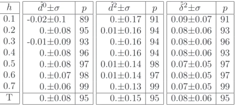
h 0.1 0.2 0.3 0.4 0.5 0.6 0.7 T ˆ d0±σ p -0.02±0.1 89 0.±0.08 95 -0.01±0.09 93 0.±0.08 96 0.±0.08 97 0.±0.07 98 0.±0.06 99 0.±0.08 95 ˆ d2±σ p 0.±0.17 91 0.01±0.16 94 0.±0.16 94 0.±0.16 94 0.01±0.14 98 0.01±0.14 97 0.±0.13 99 0.±0.15 95 ˆ δ2±σ p 0.09±0.07 91 0.08±0.06 93 0.08±0.06 96 0.08±0.06 93 0.07±0.05 97 0.08±0.05 97 0.07±0.05 99 0.08±0.06 95
Table 1. Bias and variance of the test statistics ˆd0, ˆd2 and ˆδ2 obtained on Stein’s simulations of (isotropic) fractional Brownian fields. The value p is the percentage of simulations classified as isotropic using the anisotropy test corresponding to the sta-tistics.
ν. Hence, as described in the next section, the test parameters are set experimentally using synthetic data.
3.4. Numerical Study. We generated a dataset of synthetic EFBF of size 512× 512. This dataset has two parts. The first part contains 7 subsets of 1000 isotropic fields obtained using the exact simulation technique of Stein with 7 different Hurst index values [47]. The second part contains 6 subsets of 1000 fields simulated using the spectral method [11] with various pairs of parameter values (h1, h2). We applied projection-based estimators ˆhνe (Equation (21)) with different sampling factors
ν for the estimation of Hurst indices of each simulated field in two directions (e = 1: row direction, e = 2: column direction).
We evaluated the accuracy and precision of the estimation of the Hurst index difference d by estimators ˆdν =|ˆhν
1− ˆhν2|, for ν = 0, 2, and of δ by the estimator ˆδ2. Results are reported in Tables 1.
Concerning the estimation of d, the accuracy depends on the Hurst index that is estimated. However, the precision is quite stable: it is around 0.08 when ν = 0 and 0.15 when ν = 2. We used these precision values as estimates of the standard deviation of the test statistic ˆdν. This allowed us to
set values of rejection bounds associated to the first test: c01 = 1.96∗ 0.08 ≃ 0.16 when ν = 0, and c2
1 = 1.96∗ 0.15 ≃ 0.3 when ν = 2. In the same way, we set the bound associated to the second test:
c22 = 0.2.
After setting the parameters, we applied anisotropy tests to Stein’s simulations. We reported the percentages of cases detected as isotropic are reported in Table 1. On isotropic simulations, the tests yield few errors, whatever the value of the minimal Hurst index, but results are slightly better when the Hurst index is high. The results of the first test for ν = 0 and ν = 2, and those of the second test are not significantly different: the level of confidence of the tests is about 95 percent.
We also applied the tests to the anisotropic fields simulated with the spectral method. Results are shown in Table 2. The first test for ν = 0 is more powerful than for ν = 2. When ν = 2, the test does not detect the anisotropy when Hurst index differences|h1− h2| are below 0.2 (between 74 and 84 %
of detection errors). However, the efficiency of the test is improved as differences increase. Similarly, when ν = 0, the test is not efficient when Hurst index differences are below 0.2 (between 32 and 43 % of errors). However, it becomes more reliable when differences are above 0.3 (0 % of errors). As mentioned previously, the statistic ˆd0 used in the test with ν = 0 is more biased than the one with ν = 2. However, the test yields better results with ν = 0 than with ν = 2 because statistic ˆd0 is more accurate than ˆd2.
Concerning the second test, the results obtained with ν = 2 were better than with ν = 0, due to the bias of the estimator ˆdν. Therefore, we only present results for ν = 2, when the bias of ˆdν is low.
These results are comparable to those of the first test for ν = 2.
The results obtained on anisotropic fields have to be interpreted carefully. Errors might not only be due to statistical tests. They can also be due to the simulation method itself, which in contrast to
first test (ν = 0) 0.3 0.5 0.7 0.9 0.3 98 41 43 0 0.5 97 0 0 0.7 100 32 0.9 100 first test (ν = 2) 0.3 0.5 0.7 0.9 0.3 93 74 21 6 0.5 95 84 22 0.7 99 79 0.9 99 second test (ν = 2) 0.3 0.5 0.7 0.9 0.3 56 93 36 17 0.5 89 86 17 0.7 96 78 0.9 100
Table 2. Results of the anisotropy tests obtained on spectral simulations of anisotropic fractional Brownian fields. The value p is the percentage of simulations classified into isotropic cases using the anisotropy test.
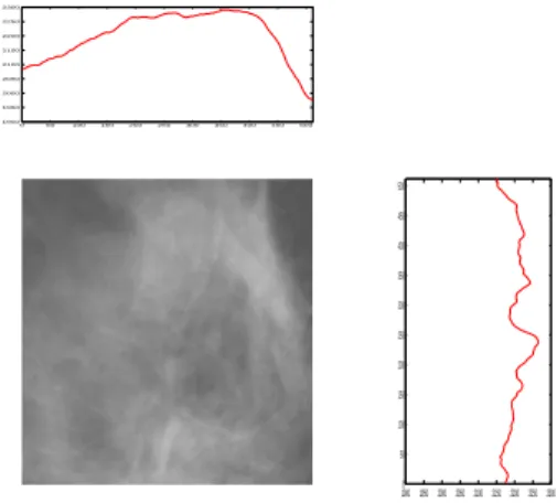
0 50 100 150 200 250 300 350 400 450 500 1900 1950 2000 2050 2100 2150 2200 2250 2300 1900 1950 2000 2050 2100 2150 2200 2250 2300 0 50 100 150 200 250 300 350 400 450 500
Figure 2. A region of interest extracted from a mammogram and its vertical and horizontal projections (case id. 83, feb05, rm).
the Stein’s method, is approximate. Hence, we cannot use these results to accurately evaluate risks of second type of tests (i.e. the risk of deciding that a field is isotropic although it is wrong).
4. Application to mammograms
4.1. Material and methods. Our database has a total of 58 cases, each case being composed of full-field digital mammograms of the left and right breasts of a woman. Images were acquired in medio-lateral oblique position using a Senographe 2000D (General Electric Medical Systems, Milwaukee, WI), with a spatial resolution of 0.1mm2 per pixel (image size: 1914x2294 pixels). Images are courtesy of the Department of Radiology of the University of Pennsylvania. In each image of the database, we extracted manually a region of interest of size 512× 512 within the densest region of the breast. As illustrated in Figure 2, we then computed the discrete row- and column-wise projections of each region of interest (Equation (19)) and the estimates of the directional Hurst indices in both directions (Equation (21), for ν = 0, 2). We also estimated the minimal Hurst index using the line-based estimators given in Equation (25). Note that in mammograms, vertical (row) and horizontal (column) directions (labeled 1 and 2) correspond to directions perpendicular and parallel to the chest wall, respectively.
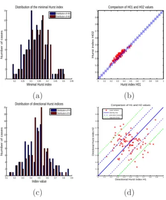
4.2. Mammogram regularity. The estimates of the minimal Hurst index we obtained using line-based estimators on the extracted regions of interest are in the interval [0.18; 0.42], with an average of 0.31 and a standard deviation of 0.05. In Figure 3 (a) and (b), we see that the line-based estimates of the minimal Hurst in both directions have equivalent empirical distributions and are approximately equal on each image. This observation is consistent with the theoretical result that shows that line-based restrictions of EFBF have same Hurst indices in all directions (see Section 3.3).
4.3. Mammogram anisotropy. In Figure 3 (c), we observe that horizontal and vertical Hurst index estimates have similar distributions. Standard deviations of horizontal and vertical Hurst indices are
0.2 0.25 0.3 0.35 0.4 0.45 0.5 0.55 0 2 4 6 8 10 12 14
Minimal Hurst index
Number of cases
Distribution of the minimal Hurst index
Distribution of H01 Distribution of H02 0 0.1 0.2 0.3 0.4 0.5 0.6 0.7 0.8 0.9 1 0 0.1 0.2 0.3 0.4 0.5 0.6 0.7 0.8 0.9 1 Hurst index H01 Hurst index H02
Comparison of H01 and H02 values
(a) (b) 0.1 0.2 0.3 0.4 0.5 0.6 0.7 0.8 0.9 0 2 4 6 8 10 12 14 16 18 20 Index value Number of cases
Distribution of directional Hurst indices
Distribution of H1 Distribution of H2 0 0.1 0.2 0.3 0.4 0.5 0.6 0.7 0.8 0.9 1 0 0.1 0.2 0.3 0.4 0.5 0.6 0.7 0.8 0.9 1
Directional Hurst index H1
Directional Hurst index H2
Comparison of H1 and H2 values case indices
identity line precision bounds rejection lines
(c) (d)
Figure 3. (a) Histograms of the minimal Hurst indices of mammograms, estimated using horizontal and vertical line-based estimators (ˆh01 and ˆh02). (b) Horizontal and
vertical line-based estimates of the minimal Hurst index on all mammograms. (c) Histograms of the horizontal and vertical Hurst indices of mammograms estimated using horizontal and vertical projection-based estimators (ˆh21 and ˆh22). (d) Horizontal and vertical projection-based estimates of the minimal Hurst index on all mammo-grams.
about 0.15 and their averages are 0.45 and 0.55, respectively. On average, the mammograms seems slightly smoother in the direction parallel to the chest wall than in the perpendicular one. Besides, ranges of minimal and directional Hurst indices are not the same. This is partly due to differences in the precision of index estimators. However, since the range difference is above the precision, this also indicates a texture anisotropy.
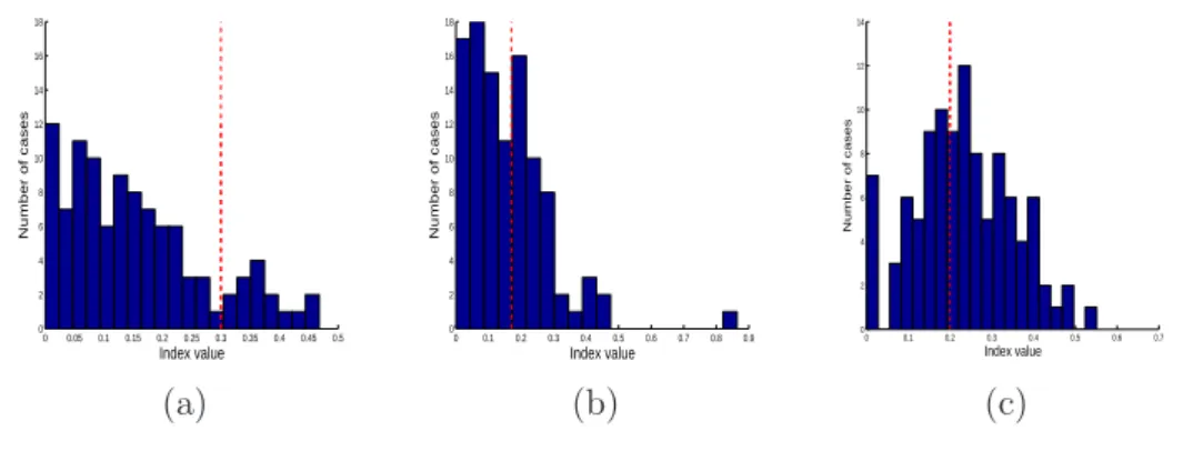
The mammogram anisotropy is further confirmed by results shown in Figures 4 (a), (b) and (c). In these figures, we plotted the histograms of estimators which are used in the different anisotropy tests, and represented the rejection bounds of these tests by red dashed lines. In Figure 4 (a), there are about 14 % of the mammograms for which the difference estimate ˆd2 is above the rejection bound. In other words, the first anisotropy test defined for ν = 2 detects very few anisotropic textures in the database. This is due to the lack of precision of the estimator ˆdν when the sampling factor ν = 2. In
Figure 4 (b), we see that the first anisotropy test for ν = 0 detects more anisotropic textures than for ν = 2: there are about 43 % of detected anisotropic cases. Recall however that anisotropic cases that have different vertical and horizontal Hurst indices cannot be detected by the first test. Such cases are better detected by the second test. Indeed, on Figure 4 (c), we observe that the second test (defined for ν = 2) detects about 60 % of anisotropic cases. All of these results have to be interpreted carefully. They do not support the conclusion that in our database, there are 60 % of anisotropic cases and 40 % of isotropic cases. They only mean that there is at least 60 % of cases which, according to the EFBF model, can be considered as anisotropic with a confidence level of 95 %.
In Figure 5, we show some examples of extracted regions of interest, with their corresponding estimator values and test decisions. Notice that in some cases (e.g. image (a)), the decision of the first test (with ν = 0) is “anisotropy” whereas the one of the second test is “weak isotropy of the second type”. This is due to the lack of precision of the estimator ˆδ2 of the second test. Let us also
0 0.05 0.1 0.15 0.2 0.25 0.3 0.35 0.4 0.45 0.5 0 2 4 6 8 10 12 14 16 18 Index value Number of cases 0 0.1 0.2 0.3 0.4 0.5 0.6 0.7 0.8 0.9 0 2 4 6 8 10 12 14 16 18 Index value Number of cases 0 0.1 0.2 0.3 0.4 0.5 0.6 0.7 0 2 4 6 8 10 12 14 Index value Number of cases (a) (b) (c)
Figure 4. Histograms of estimators (a) ˆd2 = |ˆh2
1 − ˆh22|, (b) ˆd0 = |ˆh01 − ˆh02|, and
(c) ˆδ2 =| max(ˆh21, ˆh22)− min(ˆh01, ˆh02)|. The red dashed lines represent the rejection
bounds of anisotropy tests corresponding to each estimator.
mention that in some cases (e.g. image (i)), the decision of the first test with ν = 2 is “anisotropy” whereas it is “weak isotropy of the first type” with ν = 0. Such decision difference may be an effect of the lack of accuracy of the estimator ˆd0 of the first test.
5. Discussion and conclusion
The radiographic appearance of a breast mainly depends on the distribution and relative amount of adipose and fibroglandular tissues it contains. Whereas the adipose tissues are radiologically translucent and tend to produce dark images, the fibroglandular tissues attenuate X-ray and increase the image brightness. The density of a mammogram refers to the bright image aspect caused by the presence of fibroglandular tissues in the breast. At the end of the 60’s, Wolfe put forth the idea that the breast cancer risk could be assessed from the observation of mammogram appearance and patterns [49, 48]. This pioneer work gave rise to an important medical debate. Later on, some investigators started focusing on the relationship between breast density and breast cancer risk [13, 14]. They provided the first evidence that increased breast density is associated to an increased cancer risk. This evidence was further confirmed by many subsequent epidemiological studies (see [31, 32] for an exhaustive review). These studies have shown the medical importance of mammogram density.
In many epidemiological studies, the evaluation of the density is done qualitatively by radiologists and is thus subject to inter-observer variability. Hence, early in the 90s, some investigators attempted to define quantitative and automated measurements of the density using mathematical tools; see the numerous references in the proceedings of the International Workshops on Digital Mammography [3, 26, 28, 38, 45, 51]. In particular, some of these investigators used the fractal dimension as an indicator of mammogram density [17, 18, 19]. More recently, some authors studied more deeply the stochastic nature of mammogram density by using stochastic models such as 1/f noise models related to fractional Brownian fields [16, 30, 33, 40]. As in the work presented here, these authors went into much efforts to measure model parameters on mammograms and to empirically validate models.
Measurements of Hurst-related parameters on full-field digital mammograms and film mammo-grams have been reported independently in several papers [16, 17, 19, 30, 33, 40]. Caldwell et al. [19] and Byng et al. [17, 18] used the Box counting technique to estimate the fractal dimension on the whole image. They reported estimations obtained on 70 film mammograms. Values are between 2.2 and 2.5 (with an estimated precision of 0.02), which corresponds to a minimal Hurst index between 0.46 and 0.77. Kestener et al. computed the Hurst index on small regions of size 512× 512 of film mammograms taken from the DDSM database [40]. The values of the Hurst index are in [0.20; 0.35] and [0.55; 0.75] for regions of interest with predominant adipose and dense tissues, respectively. In [33], authors used a spectral method for the estimation of the regularity coefficient β of the 1/f noise model. On 104 regions extracted from 26 full-field digital mammograms, β ∈ [1.32; 1.44], which cor-responds to H∈ [0.33; 0.42]. In another study, the same authors reported values β = [1.42, 1.51], i.e. H = [0.42; 0.51] on extracted regions of 60 film mammograms [30]. These values are in accordance
(a) (b) (c)
(d) (e) (f)
(g) (h) (i)
image case id. hˆmin hˆ21 ˆh22 dˆ2 IR dˆ0 IR δˆ2 IR
(a) 95, jun03, lm 0.32 0.33 0.25 0.07 I 0.19 A 0.01 I (b) 76, oct03, lm 0.36 0.38 0.43 0.05 I 0.05 I 0.07 I (c) 74, dec04, lm 0.39 0.50 0.32 0.18 I 0.01 I 0.11 I (d) 86, mar05, lm 0.33 0.35 0.44 0.05 I 0.28 A 0.11 I (e) 83, feb05, lm 0.37 0.52 0.45 0.08 I 0.17 A 0.15 I (f) 85, mar05, lm 0.26 0.48 0.45 0.03 I 0.15 A 0.22 I (g) 73, dec04, lm 0.35 0.72 0.55 0.17 I 0.22 A 0.37 A (h) 83, feb05, rm 0.32 0.73 0.47 0.26 A 0.01 I 0.41 A (i) 85, mar05, rm 0.26 0.39 0.75 0.36 A 0.14 I 0.49 A Figure 5. Some regions of interest extracted from mammograms with their estimated indices. Columns IR give the decisions of the anisotropy tests based on the estimators
ˆ
d0, ˆd2 and ˆδ2 (A=anisotropic, I=isotropic).
with those obtained independently in [16]. The values we obtained using the line-based estimators are close to those obtained by Heine et al. [33] on full-field digital mammograms: they are slightly lower probably due to (a) the estimation technique difference and (b) to the selection of the regions of interest which in our study can be of low density.
Similarly to [16, 30, 33], our experiments confirm the relevance of fractional Brownian models for the characterization of mammogram density. However, they also reveal that the isotropy assumption which is behind the mammogram modeling of [16, 30, 33] is not valid in many cases: around 60 percent of the mammogram textures we studied could be considered as anisotropic with a high level of confidence. Hence, we conclude that the EFBF model is more realistic and relevant than a simple fractional Brownian field model for the description of mammogram textures.
From a medical point of view, this conclusion suggests the anisotropy should be taken into account for the analysis of mammogram density and the evaluation of breast cancer risk. However, the establishment of a relationship between anisotropy and breast cancer risk is beyond the scope of this paper. The present research can be seen as an encouraging starting point for future medical
investigations. Up to now, we have shown that the EFBF model enables to extract some significant density features which are not captured by the usual fractional Brownian field model. We have also constructed a mathematical methodology for analyzing those features. In collaboration with radiologists, we plan to further evaluate the medical relevance of density anisotropy for the assessment of breast cancer risk and for the analysis of lesion detectability.
The interest of this paper is not restricted to results concerning the mammogram application. The methodology we proposed for characterizing and testing the anisotropy of fractional Brownian textures is generic. We believe that this methodology could be useful in many medical applications, such as the analysis of osteoporosis from bone radiographs. The methodology includes some original statistical tests of anisotropy, based on estimates of directional Hurst indices. We showed a new theoretical result about the estimator convergence, which gives a mathematical foundation to the construction of those tests. The statistical tests were also validated on simulated data.
Appendix A. Proof of Theorem 3.1
Proof. The key point of the proof relies on the introduction of auxiliary estimators. Let θ1 = (0, 1)
and θ2 = (1, 0). Let N, u ≥ 1 and let us denote ZN,u(θ1), respectively ZN,u(θ2), the second-order
increments of RρX(θ1, t) = RRX(s, t)ρ(s)ds, respectively RρX(θ2, t) = RRX(t, s)ρ(s)ds, as defined
by (11). We consider estimators defined from generalized quadratic variations VN,u(θ1) and VN,u(θ2)
of ZN,u(θ1) and ZN,u(θ2), according to (12), by
TN,u(θ1) = VN,u(θ1)/E (VN,u(θ1)) and TN,u(θ2) = VN,u(θ2)/E (VN,u(θ2)) .
Without loss of generality we can also assume that h1= h(θ1)≤ h2= h(θ2). Usual computations on
generalized quadratic variations lead to TN,u(θe) −→
N→+∞1 a. s. with
√
N (TN,u(θe)− 1) −→
N→+∞N (0, σu,u(he)),
for e, u∈ {1, 2}, where for v ∈ {1, 2}
(28) σu,v(he) = Cu,v µ he+ 1 2 ¶ /(uv)2he+1E µ he+ 1 2 ¶2 , with Cu,v(H) = 4P p∈Z ¡R
Re−ipξ(1− e−iuξ)2(1− eivξ)2|ξ|−2H−1dξ
¢2
= Cv,u(H) and
E(H) =RR¯¯(e−iξ− 1)2¯¯2|ξ|−2H−1dξ, which are finite positive constants for H ∈ (0, 2) (see Theorem
2.3 of [11] for instance). It is straightforward that the vector (TN,u(θe))1≤e,u≤2converges to (1)1≤e,u≤2
almost surely as N → +∞. Let us prove the asymptotic normality. Let us remark that for any
(ae,u)1≤e,u≤2 positive number one can write
X 1≤e,u≤2 ae,u(TN,u(θe)− 1) = 1 E(VN,1(θ1)) X 1≤e,u≤2 ae,u E(VN,1(θ1))
E(VN,u(θe))(VN,u(θe)− E (VN,u(θe))) .
From Proposition 1.1 of [11] we get ae,u E(VN,1(θ1)) E(VN,u(θe)) = be,uN −2(h1−he) µ 1 + O N→+∞(N −1)¶,
with be,u= ae,u
E(h1+ 1 2) E(he+ 1 2) u−2he−1 ≥ 0. Let us write X 1≤e,u≤2
be,uN−2(h1−he)(VN,u(θe)− E (VN,u(θe))) d = n(N ) X k=1 λk,N¡ε2k,N− 1 ¢ ,
where n(N ) = 4N− 8, (εk,N)1≤k≤n(N ) is a sequence of independent standard Gaussian variables and
(λk,N)1≤k≤n(N ) are the eigenvalues of the covariance matrix of
s be,uN−2(h1−he) N − 2u + 1 ZN,u(θe)(p); 1≤ e, u ≤ 2, 0 ≤ p ≤ N − 2u . Let s2N = Var X 1≤e,u≤2
be,uN−2(h1−he)(VN,u(θe)− E (VN,u(θe)))
. Following a Lindeberg condition [23] we obtain
(29) s−1N X
1≤e,u≤2
be,uN−2(h1−he)(VN,u(θe)− E (VN,u(θe))) −→
N→+∞N (0, 1),
as soon as max
1≤k≤n(N )|λk,N| =N→+∞o (sN). On the one hand, an upper bound for 1≤k≤n(N )max |λk,n| is given
by
c1 max
1≤e,u≤2 0≤p≤N −2umax
X 1≤e′,u′≤2 N−(2h1−he′−he+1) N−2u′ X p′=0 ¯
¯Cov¡ZN,u(θe)(p), ZN,u′(θe′)(p′)¢¯¯ ,
for some positive constant c1. According to Proposition 1.2 of [11], one can find c2 > 0 such that for
any 1≤ u, u′≤ 2,
N−2u′
X
p′=0
¯
¯Cov¡ZN,u(θe)(p), ZN,u′(θe)(p′)
¢¯
¯ ≤ c2N−2he−1log(N ),
for any 0 ≤ p ≤ N − 2u. There remains to consider the covariance terms between ZN,u(θ1) and
ZN,u′(θ2). Using the spectral representation of the random field X we get
Cov¡ZN,u(θ1)(p), ZN,u′(θ2)(p′)
¢ = Z R2 eipξ2N e−i p′ξ1 N (1− eiu ξ2 N)2(1− e−iu′ ξ1N)2f (ξ)bρ(ξ1)bρ(ξ2)dξ,
where bρ(ξe) = RReisξeρ(s)ds is the Fourier transform of the window function, which belongs to the
Schwartz class since ρ does. Therefore ¯
¯Cov¡ZN,u(θ1)(p), ZN,u′(θ2)(p′)
¢¯ ¯ ≤ c3N−4, with c3 = (uu′)2 Z R2 ξ22ξ12f (ξ)bρ(ξ1)bρ(ξ2)dξ < +∞.
As a result, for any 1≤ u, u′ ≤ 2 and e 6= e′,
N−2u′
X
p′=0
¯
¯Cov¡ZN,u(θe)(p), ZN,u′(θe′)(p′)
¢¯
¯ ≤ c3N−3,
such that this part will not interfere with the previous asymptotics. Therefore, max
1≤k≤n(N )|λk,N| =N→+∞O (N
−2h1−2log(N )).
On the other hand, since (ae,u)1≤e,u≤2 are positive numbers, using the fact that
Cov¡ZN,u(θe)(p)2, ZN,u′(θe′)(p′)2
¢ = 2Cov¡ZN,u(θe)(p), Ze′,u′(θe′)(p′) ¢2 ≥ 0, we get s2N ≥ X 1≤e,u≤2 b2e,uN−4(h1−he)Var (V N,u(θe))≥ c4N−4h1−3,
from Proposition 1.2 of [11], for some c4 > 0. Then (29) holds. Let us remark that E(VN,1sN(θ1)) = √ N µp aΓ(h1, h2)at+ O N→+∞(N −1) ¶ with a = ( a1,1 a1,2 a2,1 a2,2 ) and Γ(h1, h2) = σ1,1(h1) σ1,2(h1) 0 0 σ2,1(h1) σ2,2(h1) 0 0 0 0 σ1,1(h2) σ1,2(h2) 0 0 σ2,1(h2) σ2,2(h2) . Hence we get an asymptotic normality for X
1≤e,u≤2
ae,u(TN,u(θe)− 1), for any set (ae,u)1≤e,u≤2 of
positive numbers. Using tightness criterion and uniqueness of the limit law we can claim that √
N (TN,u(θe)− 1)1≤e,u≤2 −→
N→+∞N (0, Γ(h1, h2)).
By Taylor Formula for the function
g(x1,1, x1,2, x2,1, x2,2) = log µ x1,2 x1,1 ¶ − log µ x2,2 x2,1 
(see Theorem 3.3.11 in [24] for instance) we get that almost surely log³TN,2(θ1)
TN,1(θ1) ´ −log³TN,2(θ2) TN,1(θ2) ´ −→ N→+∞ 0 with √N³log³TN,2(θ1) TN,1(θ1) ´ − log³TN,2(θ2) TN,1(θ2) ´´ d −→ N→+∞ N ¡ 0, a0Γ(h1, h2)at0 ¢ for a0 = ∇g(1, 1, 1, 1) = ( −1 1 1 −1 ).
From (14), with ˆh1 = ˆh(θ1) and ˆh2 = ˆh(θ2), we have
2 log(2)³ˆh1− ˆh2 ´ = log µE (VN,2(θ1)) E(VN,1((θ1)) ¶ +log µ TN,2(θ1) TN,1(θ1) ¶ − µ log µE (VN,2(θ2)) E(VN,1(θ2)) ¶ + log µ TN,2(θ2) TN,1(θ2) ¶¶ , with for e∈ {1, 2}, by Proposition 1.1 of [11],
E(VN,2(θe)) E(VN,1(θe)) = 2 2he+1 µ 1 + o N→+∞ ³ 1/√N´¶. Then, ˆ h1− ˆh2= h1− h2+ 1 2 log(2) µ log µT N,2(θ1) TN,1(θ1) ¶ − log µT N,2(θ2) TN,1(θ2) ¶¶ + o N→+∞ ³ 1/√N´, such that, with γ2(h1, h2) = a
0Γ(h1,h2)at0 4 log(2)2 , ˆ h1− ˆh2 −→ N→+∞h1− h2 a.s., with √ N³hˆ1− ˆh2− (h1− h2) ´ d −→ N→+∞N ¡ 0, γ2(h1, h2)¢. ¤ Acknowledgments. The authors are grateful to Dr. Bakic and Dr. Maidment (University of Penn-sylvania) for offering them the opportunity to study full-field digital mammograms acquired in their department of Radiology. This work was supported by the grant “mipomodim” ANR-05-BLAN-0017 of the ”Agence National pour la Recherche”.
References
[1] P. Abry, P. Gonçalves, and F. Sellan. Wavelet spectrum analysis and 1/f processes. In Lecture Notes in Statistics, volume 103, pages 15–30. Springer-Verlag, 1995.
[2] R. J. Adler. The Geometry of Random Field. John Wiley & Sons, 1981.
[3] S. Astley et al., editors. Proc. of the 8th International Workshop on Digital Mammography, LNCS, 4046, Manch-ester, UK, June 2004. Springer.
[4] A. Ayache, A. Bonami, and A. Estrade. Identification and series decomposition of anisotropic Gaussian fields. In Proc. of the Catania ISAAC05 congress, 2005.
[5] J. M. Bardet, G. Lang, G. Oppenheim, et al. Semi-parametric estimation of the long-range dependence parameter: a survey. In Theory and applications of long-range dependence, pages 557–577. Birkhauser Boston, 2003.
[6] A. Begyn. Asymptotic expansion and central limit theorem for quadratic variations of Gaussian processes. Bernoulli, 13(3):712–753, 2007.
[7] C.L. Benhamou, S. Poupon, E. Lespessailles, et al. Fractal analysis of radiographic trabecular bone texture and bone mineral density. J. Bone Miner. Res., 16(4):697–703, 2001.
[8] D. Benson, M. M. Meerschaert, B. Bäumer, and H. P. Scheffler. Aquifer operator-scaling and the effect on solute mixing and dispersion. Water Resour. Res., 42:1–18, 2006.
[9] J. Beran. Statitics for long-memory processes. Chapman Hall London, 1994.
[10] H. Biermé, M. M. Meerschaert, and H. P. Scheffler. Operator scaling stable random fields. Stoch. Proc. Appl., 117(3):312–332, 2007.
[11] H. Biermé and F. Richard. Estimation of anisotropic gaussian fields through radon transform. ESAIM: Probab. Stat., 12(1): 30–50, 2008.
[12] A. Bonami and A. Estrade. Anisotropic analysis of some Gaussian models. J. Fourier Anal. Appl., 9:215–236, 2003. [13] N.F. Boyd, B. O’Sullivan, J.E. Campbell, et al. Mammographic signs as risk factors for breast cancer. Br. J.
Cancer, 45:185–193, 1982.
[14] J. Brisson, F. Merletti, N.L. Sadowsky, et al. Mammographic features of the breast and breast cancer risk. Am. J. Epidemiol., 115(3):428–437, 1982.
[15] B. Brunet-Imbault, G. Lemineur, C. Chappard, et al. A new anisotropy index on trabecular bone radiographic images using the fast Fourier transform. BMC Med. Imaging, 5(4), 2005.
[16] A. Burgess, F. Jacobson, and P. Judy. Human observer detection experiments with mammograms and power-law noise. Med. Phys., 28(4):419–437, 2001.
[17] J. Byng, N. N. Boyd, and E. others Fishell. Automated analysis of mammographic densities. Phys. Med. Biol., 41:909–923, 1996.
[18] J. Byng, M. Yaffe, G. Lockwood, et al. Automated analysis of mammographic densities and breast carcinoma risk. Cancer, 80(1):66–74, 1997.
[19] C. Caldwell, S. Stapleton, D. Holdsworth, et al. Characterisation of mammographic parenchymal patterns by fractal dimension. Phys. Med. Biol., 35(2):235–247, 1990.
[20] C.-C. Chen, J. Daponte, and M. Fox. Fractal feature analysis and classification in medical imaging. IEEE Trans. Pattern. Anal. Mach. Intell., 8(2):133–142, 1989.
[21] J. F. Coeurjolly. Inférence statistique pour les mouvements browniens fractionnaires et multifractionnaires. PhD thesis, University Joseph Fourier, 2000.
[22] G. Cross and A. Jain. Markov random field texture models. IEEE Trans. Pattern. Anal. Mach. Intell., 5(1):25–39, 1983.
[23] M. Czörgö and P. Révész. Strong approximation in probability and statistics. Academic Press, 1981. [24] D. Dacunha-Castelle and M. Duflo. Probabilités et statistiques, volume 2. Masson, 1983.
[25] S. Davies and P. Hall. Fractal analysis of surface roughness by using spatial data. J. R. Stat. Soc. Ser. B, 61:3–37, 1999.
[26] K. Doi et al., editors. Proc. of the 3rd International Workshop on Digital Mammography, Chicago, USA, June 1996. Elsevier Science.
[27] K. J. Falconer. Fractal Geometry. John Wiley & Sons, 1990.
[28] A.G. Gale et al., editors. Proc. of the 2nd International Workshop on Digital Mammography, York, England, July 1994. Elsevier Science.
[29] B. Grosjean and L. Moisan A-contrario detectability of spots in textured backgrounds J. Math. Imaging Vis., 33(3):313–337, 2009.
[30] J. Heine, S. Deine, R. Velthuizen, et al. On the statistical nature of mammograms. Med. Phys., 26(11):2254–2269, 1999.
[31] J. Heine and P. Malhorta. Mammographic tissue, breast cancer risk, serial image analysis, and digital mammog-raphy: serial breast tissue change and related temporal influences. Acad. Radiol., 9:317–335, 2002.
[32] J. Heine and P. Malhorta. Mammographic tissue, breast cancer risk, serial image analysis, and digital mammog-raphy: tissue and related risk factors. Acad. Radiol, 9:298–316, 2002.
[33] J. Heine and R. Velthuizen. Spectral analysis of full field digital mammography data. Med. Phys., 29(5):647–661, 2002.
[34] J. Istas. Identifying the anisotropical function of a d-dimensional Gaussian self-similar process with stationary increments. Stat. Inference Stoch. Process., 10(1):97–106, 2007.
[35] J. Istas and G. Lang. Quadratic variations and estimation of the local Holder index of a Gaussian process. Ann. Inst. Henri Poincaré, Probab. Statist., 33(4):407–436, 1997.
[36] R. Jennane, R. Harba, G. Lemineur, et al. Estimation of the 3D self-similarity parameter of trabecular bone from its projection. Med. Image Anal., 11:91–98, 2007.
[37] A. Kamont. On the fractional anisotropic Wiener field. Probab. Math. Statist., 16:85–98, 1996.
[38] N. Karssemeijer et al., editors. 4th International Workshop on Digital Mammography, Nijmegen, The Netherlands, June 1998. Kluwer Academic.
[39] J. T. Kent and A. T. A. Wood. Estimating the fractal dimension of a locally self-similar Gaussian process by using increments. J. R. Stat. Soc. Ser. B, 59(3):679–699, 1997.
[40] P. Kestener, J.-M. Lina, P. Saint-Jean, et al. Wavelet-based multifractal formalism to assist in diagnosis in digitized mammograms. Image Anal. Stereol., 20:169–174, 2001.
[41] A. N. Kolmogorov. Wienersche Spiralen und einige andere interessante Kurven in Hilbertsche Raum.. C. R. (Dokl.) Acad. Sci. URSS,26:115–118,1940.
[42] S. Leger. Analyse stochastique de signaux multi-fractaux et estimations de paramètres. PhD thesis, Université d’Orléans, 2000.
[43] T. Lundahl, W.J. Ohley, S.M. Kay, and R. Siffe. Fractional brownian motion: a maximum likelihood estimator and its application to image texture. IEEE Trans. Med. Imaging, 5(3):152–161, 1986.
[44] B. B. Mandelbrot and J. Van Ness. Fractional Brownian motion, fractionnal noises and applications. SIAM Rev., 10:422–437, 1968.
[45] H.-O. Peitgen, editor. 6th International Workshop on Digital Mammography, Bremen, Germany, June 2002. Springer.
[46] A. Pentland. Fractal-based description of natural scenes. IEEE Trans. Pattern. Anal. Mach. Intell., 6:661–674, 1984.
[47] M. L. Stein. Fast and exact simulation of fractional Brownian surfaces. J. Comput. Graph. Stat., 11(3):587–599, 2002.
[48] J.N. Wolfe. Ducts as a sole indicator of breast carcinoma. Radiology, 89:206–210, 1967.
[49] J.N. Wolfe. A study of breast parenchyma by mammography in the normal woman and those with benign and malignant disease. Radiology, 89:201–205, 1967.
[50] Y. Xiao. Sample path properties of anisotropic Gaussian random fields. In A Minicourse on Stochastic Partial Differential Equations, (D. Khoshnevisan and F. Rassoul-Agha, editors), Lecture Notes in Math. 1962, pp. 145– 212, Springer, New York, 2009.
[51] M. Yaffe et al., editors. Proc. of the 5th International Workshop on Digital Mammography, Toronto, Canada, June 2000. Medical Physics Publishing.
University Paris Descartes, Laboratory MAP5, CNRS UMR 8145, 45, rue des Saints-Pères, 75006 PARIS, FRANCE.