Dynamics of the terrestrial biosphere, climate and atmospheric CO₂ concentration during interglacials: a comparison between Eemian and Holocene

HAL Id: hal-00298058

https://hal.archives-ouvertes.fr/hal-00298058

Submitted on 22 Nov 2006

HAL is a multi-disciplinary open access

archive for the deposit and dissemination of

sci-entific research documents, whether they are

pub-lished or not. The documents may come from

teaching and research institutions in France or

abroad, or from public or private research centers.

L’archive ouverte pluridisciplinaire HAL, est

destinée au dépôt et à la diffusion de documents

scientifiques de niveau recherche, publiés ou non,

émanant des établissements d’enseignement et de

recherche français ou étrangers, des laboratoires

publics ou privés.

atmospheric CO2 concentration during interglacials: a

comparison between Eemian and Holocene

G. Schurgers, U. Mikolajewicz, M. Gröger, E. Maier-Reimer, M. Vizcaíno, A.

Winguth

To cite this version:

G. Schurgers, U. Mikolajewicz, M. Gröger, E. Maier-Reimer, M. Vizcaíno, et al.. Dynamics of the

terrestrial biosphere, climate and atmospheric CO2 concentration during interglacials: a comparison

between Eemian and Holocene. Climate of the Past, European Geosciences Union (EGU), 2006, 2

(2), pp.205-220. �hal-00298058�

www.clim-past.net/2/205/2006/

© Author(s) 2006. This work is licensed under a Creative Commons License.

of the Past

Dynamics of the terrestrial biosphere, climate and atmospheric CO

2

concentration during interglacials: a comparison between Eemian

and Holocene

G. Schurgers1,*, U. Mikolajewicz1, M. Gr¨oger1, E. Maier-Reimer1, M. Vizca´ıno1,**, and A. Winguth2 1_{Max Planck Institute for Meteorology, Bundesstrasse 53, 20146 Hamburg, Germany}

2_{Center for Climatic Research, Department of Atmospheric and Oceanic Sciences, University of Wisconsin, USA} *_{present affiliation: Department of Physical Geography and Ecosystem Analysis, Lund University, Sweden}

**_{present affiliation: Department of Geography and Center for Atmospheric Sciences, University of California, Berkeley,}

USA

Received: 29 June 2006 – Published in Clim. Past Discuss.: 17 July 2006

Revised: 17 October 2006 – Accepted: 8 November 2006 – Published: 22 November 2006

Abstract. A complex earth system model (atmosphere and

ocean general circulation models, ocean biogeochemistry and terrestrial biosphere) was used to perform transient simu-lations of two interglacial sections (Eemian, 128–113 ky B.P., and Holocene, 9 ky B.P.–present). The changes in terrestrial carbon storage during these interglacials were studied with respect to changes in the earth’s orbit. The effects of different climate factors on changes in carbon storage were studied in offline experiments in which the vegetation model was forced only with temperature, hydrological parameters, radiation, or CO2concentration from the transient runs.

The largest anomalies in terrestrial carbon storage were caused by temperature changes. However, the increase in storage due to forest expansion and increased photosynthe-sis in the high latitudes was nearly balanced by the decrease due to increased respiration. Large positive effects on carbon storage were caused by an enhanced monsoon circulation in the subtropics between 128 and 121 ky B.P. and between 9 and 6 ky B.P., and by increases in incoming radiation during summer for 45◦ _{to 70}◦_{N compared to a control simulation}

with present-day insolation.

Compared to this control simulation, the net effect of these changes was a positive carbon storage anomaly in the terrestrial biosphere of about 200 Pg C for 125 ky B.P. and 7 ky B.P., and a negative anomaly around 150 Pg C for 116 ky B.P. Although the net increases for Eemian and Holocene were rather similar, the magnitudes of the pro-cesses causing these effects were different. The decrease in terrestrial carbon storage during the experiments was the main driver of an increase in atmospheric CO2concentration

during both the Eemian and the Holocene.

Correspondence to: G. Schurgers

([email protected])

1 Introduction

The record of atmospheric CO2concentrations as observed

in ice cores (Inderm¨uhle et al., 1999) displays a rising trend for the last 8000 years, from around 260 ppm at 8 ky B.P. to around 280 ppm for the pre-industrial era. Several different factors have been proposed as cause or contributor to this rise: natural changes in carbon storage on land (Inderm¨uhle et al., 1999) or in the oceans (Broecker and Clark, 2003), or by early anthropogenic land cover and land use change (Ruddiman, 2003).

A few studies with transient simulations have been per-formed for the Holocene with models less complex than the one presented here: Brovkin et al. (2002) performed simula-tions with the earth system model of intermediate complex-ity CLIMBER, and Joos et al. (2004) performed simulations with the dynamic global vegetation model LPJ coupled to an impulse-response function model for the ocean carbon cycle based on the HILDA ocean model.

Both Brovkin et al. (2002) and Joos et al. (2004) obtain a reasonable reconstruction of the increase in atmospheric CO2

concentrations over the last 8000 years. However, the causes for this increase differ between these studies. In the study of Brovkin et al. (2002) the increase of the CO2concentration is

driven by a decrease of terrestrial carbon storage of 90 Pg C over the last 8000 years combined with an external forcing of increased carbonate sedimentation, while in the study by Joos et al. (2004) it is driven by a decrease of oceanic carbon by sediments and ocean surface heating. In the latter study, the terrestrial biosphere shows no clear uptake or release of carbon for the last 8000 years. A reconstruction of terrestrial carbon storage for the Holocene by Kaplan et al. (2002) had similar results as the study by Joos et al. (2004): during the

early Holocene simulated terrestrial carbon storage increased markedly, with a continued slight increase after 8 ky B.P.

A few reconstructions of global vegetation distribution for the Holocene have been synthesized. The BIOME 6000 project (Prentice and Webb III, 1998; Prentice et al., 2000) provide a reconstruction for 6 ky B.P. based on pollen data, and Adams and Faure (1997) published reconstructions for 8 and 5 ky B.P. based on several sources. The most important consistent feature of mid-Holocene vegetation distribution in these and other studies is an increase of vegetation in mon-soon areas in the subtropics of the northern hemisphere.

In the study presented here, a complex earth system model was applied to reconstruct the global carbon cycle of the Eemian and the Holocene. Carbon storage in the terrestrial biosphere and its contribution to the atmospheric CO2

con-centration were analysed. The changes in terrestrial carbon storage were traced back to certain climatic factors.

2 Method

2.1 Model

A complex earth system model, consisting of general cir-culation models for atmosphere and ocean, an ocean bio-geochemistry model, and a dynamic vegetation model, was used to perform transient simulations of two interglacials. The general circulation model for atmosphere and ocean, ECHAM3-LSG, was used in a coupled mode before for long-term experiments, both regarding paleoclimate (Mikolajew-icz et al., 2003) and anthropogenic warming (Voss and Miko-lajewicz, 2001). The carbon cycle within the earth sys-tem model was represented with the dynamic global veg-etation model LPJ (Sitch et al., 2003) and a marine bio-geochemistry model based on HAMOCC3 (Maier-Reimer, 1993), described in Winguth et al. (2005) and Mikolajewicz et al. (2006). The dynamic global vegetation model calcu-lates the occurrence of ten plant functional types (PFTs), and within these PFTs carbon is allocated between four biomass pools. Each PFT contains three litter pools, and each gridcell (which can contain more than one PFT) contains two soil carbon pools. The ocean biogeochemistry model simulates the distribution of the main components for the carbon cycle, including CO2, particulate organic carbon and CaCO3. A

se-diment module was inserted to account for long-term storage or dissolution of sediments. CO2is treated prognostically in

the earth system model, changes in carbon storage on land and in the ocean influence the atmospheric CO2

concentra-tion, which is modelled as a well-mixed box.

The land surface conditions for the atmosphere were adapted according to changes in the vegetation (Schurgers, 2006). A version of the earth system model in which the ice sheets were treated interactively was described in Winguth et al. (2005) and Mikolajewicz et al. (2006), however, for the

study presented here the ice sheets were fixed at present-day conditions.

In order to enable long paleoclimate experiments with this complex model, the resolution of the components is rela-tively low: the atmosphere and the vegetation model run on a T21 grid (roughly 5.6◦×5.6◦), the ocean and ocean biogeo-chemistry run on a Arakawa E-grid (effectively 4.0◦×4.0◦). A modified version of the periodically-synchronous coupling technique by Sausen and Voss (1996) was applied, using fixed fluxes at the surface rather than an energy balance model. It was described in detail in Mikolajewicz et al. (2006). Both experiments were started from a pre-industrial control simulation, followed by a 1000 year spinup with insolation according to 129–128 ky B.P. (Eemian) and 10– 9 ky B.P. (Holocene). The length of this spinup is too small to bring all components, especially the ocean and the marine carbon cycle, in equilibrium. However, neither the ocean nor the marine carbon cycle were, in reality, in equilibrium. This causes uncertainties for the initial state of the simulated sys-tem.

Not incorporated in the model were peatlands, rock weath-ering dynamics and pedogenesis, tectonic effects and coral reefs. Peatlands are not simulated by the dynamic vegeta-tion model LPJ. Weathering is prescribed at a constant rate, roughly equal to the average sedimentation rate of the control simulation. In principle we should consider the evolution of coral reefs, too; there are, however, very large uncertainties about their dynamics so that a reliable modeling up to now is excluded. These processes might be important components of the global carbon cycle on the timescales addressed here. The dynamic vegetation model LPJ was designed for stud-ies with timescales of ∼100 years. On longer timescales, as applied here, especially the processes regarding soil organic matter formation might become important, and the relatively simple representation in LPJ is a limitation of the model for these timescales.

2.2 Biome descriptions

As a tool for evaluation of the vegetation distribution, a scheme was developed to represent the regular output of the vegetation model in so-called biomes or macro-ecosystems. In order to compare the modelled distribution of plant func-tional types with vegetation reconstructions for the past, the combinations of plant functional types as were simulated by LPJ are converted into seven biome classes. Several schemes have been described in literature, the classes that are pro-posed here are (1) able to present the major conversions that take place on longer time scales, (2) are structured in a way that is understandable and (3) can be derived from the LPJ output, without putting in too much uncertainty, but with enough distinction between them to show shifts of vegeta-tion over long time scales. The scheme that is used here uses the fractions of coverage from the ten plant functional types from the output of the vegetation model, together with the

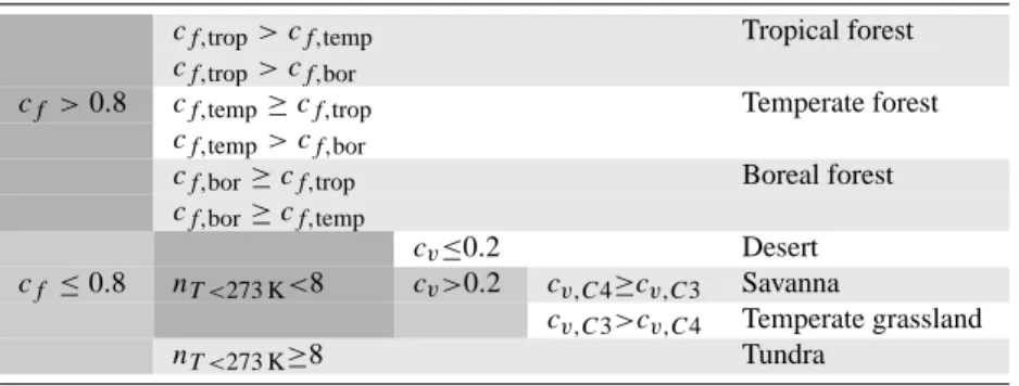
Table 1. Conditions used to distinguish biomes.

cf,trop> cf,temp Tropical forest

cf,trop> cf,bor

cf >0.8 cf,temp≥cf,trop Temperate forest

c_f,temp> cf,bor

cf,bor≥cf,trop Boreal forest

cf,bor≥cf,temp

cv≤0.2 Desert

cf ≤0.8 nT <273 K<8 cv>0.2 cv,C4≥cv,C3 Savanna

cv,C3>cv,C4 Temperate grassland

nT <273 K≥8 Tundra

cf forest fraction (sum of cover of all tree PFTs);

c_f,troptropical forest fraction (sum of cover of all tropical tree PFTs);

cf,temptemperate forest fraction;

c_f,borboreal forest fraction;

cvvegetation fraction (sum of cover of all PFTs);

nT <273 Knumber of months with average soil temperature below 273 K;

cv,C4C4herbs fraction;

cv,C3C3herbs fraction.

Table 2. Overview of the experiments.

CTL coupled control simulation with present-day insolation

EEM coupled simulation with transient Eemian insolation (128–113 ky B.P.) HOL coupled simulation with transient Holocene insolation (9 ky B.P.–present)

EEM tem vegetation run with simulated control climate and Eemian temperatures (air, surface and soil temperatures) EEM hyd vegetation run with simulated control climate and Eemian hydrological parameters (soil moisture, precipitation) EEM rad vegetation run with simulated control climate and Eemian radiation

EEM co2 vegetation run with simulated control climate and Eemian atmospheric CO2concentration

HOL tem vegetation run with simulated control climate and Holocene temperatures (air, surface and soil temperatures) HOL hyd vegetation run with simulated control climate and Holocene hydrological parameters (soil moisture, precipitation) HOL rad vegetation run with simulated control climate and Holocene radiation

HOL co2 vegetation run with simulated control climate and Holocene atmospheric CO2concentration

soil temperature from the land surface scheme of the atmo-sphere model. The distribution is explained in Table 1. 2.3 Experiments

Long integrations were performed with the complex earth system model for the Eemian (128 ky B.P.–113 ky B.P.) and the Holocene (9 ky B.P.–present), for which insolation changes were prescribed according to Berger (1978). A con-trol simulation of 10 000 years was performed with present-day insolation. CO2was treated prognostically in the earth

system model, changes in carbon storage on land and in the ocean influence the atmospheric CO2concentration. For the

control run, the atmospheric CO2concentration was 279 ppm

on average. Ice sheets were fixed at their present-day state. Both experiments were started from a pre-industrial

con-trol simulation, followed by a 1000 year spinup with insola-tion according to 129–128 ky B.P. (Eemian) and 10–9 ky B.P. (Holocene).

In addition to these two coupled integrations, climate data from these experiments were used to perform experiments with the vegetation model in an offline mode. Experiments were performed based on the simulated control climate, with temperatures, radiation, hydrological parameters or pCO2

from the Eemian or Holocene experiments, to determine which parameters influence the distribution and carbon stor-age of vegetation most. An overview of the experiments is shown in Table 2.

114 116 118 120 122 124 126 128 286 286.2 286.4 286.6 286.8 287 temperature (K) CTL EEM 0 2 4 6 8 286 286.2 286.4 286.6 286.8 287 CTL HOL 114 116 118 120 122 124 126 128 0.5 0.505 0.51 0.515 0.52 evaporation (10 6 km 3 y -1 ) 0 2 4 6 8 0.5 0.505 0.51 0.515 0.52 114 116 118 120 122 124 126 128 26 28 30 32 34

sea ice cover (10

6 km 2 ) 0 2 4 6 8 26 28 30 32 34 Eemian Holocene time (ky B.P.) (c) (b) (a)

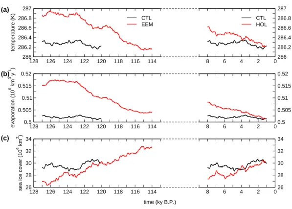
Fig. 1. Time series of (a) globally averaged near-surface air temperature, (b) global evaporation, and (c) global sea ice cover for the Eemian and the Holocene experiments (EEM and HOL) and the control simulation (CTL). Shown are 2 ky running means.

3 Results

Results from climate change, changes in vegetation distribu-tion and changes in terrestrial carbon storage in the experi-ments are described below.

3.1 Climate change

Due to changes in the temporal and spatial distribution of in-coming solar radiation, climate changed both in its annual mean state, and in its annual cycle. At the beginning of both the Eemian and the Holocene experiments, global tem-peratures are higher than the control experiment (0.5 K for 128 ky B.P. and 0.2 K for 9 ky B.P.; Fig. 1a). During the two interglacials, global temperature decreases towards the pre-industrial control average. For the Eemian, from 117 ky B.P. onwards global temperature is lower than for the control simulation. Increased temperatures are accompanied by in-creased evaporation, with a maximum of 15×103km3y−1 (3.0%) for the Eemian and 6×103km3y−1 (1.2%) for the Holocene compared to the control value (Fig. 1b). Global sea ice cover shows a course consistent with global temperature, which is mainly resulting from the northern hemisphere: for the beginning of the insolation experiments sea ice cover is

lower than for the control simulation by 2 to 3×106km2, and ice cover increases during the experiments (Fig. 1c). 3.2 Vegetation distribution

3.2.1 Simulated changes

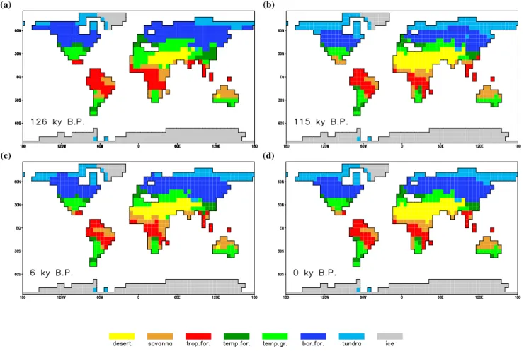
The distribution of vegetation for selected time slices in these periods is shown in Fig. 2, using the biome descriptions pre-sented in Sect. 2.2. For present-day (Fig. 2d), the pattern matches quite well with what is considered as “potential nat-ural” vegetation for most parts of the world. Remarkable de-viations are simulated for the Amazon region, which is dom-inated by savanna in the simulation, Europe, where boreal forest is simulated rather than temperate forest, and Aus-tralia, which lacks large desert areas. These deviations are caused by the simulated control climate: the high latitudes are in general too cold, and the Amazon region is too dry.

For 6 ky B.P. (Fig. 2c), both at the northern and the south-ern boundary of the Sahara desert, and in the South Asian deserts, vegetation expands compared to the control simula-tion, and the area of deserts decreases. At the high latitudes of North America, and to a lesser extent the high latitudes of east Asia, boreal forest expands compared to the control simulation. For 126 ky B.P. (Fig. 2a), these effects are even

(a) (b)

(c) (d)

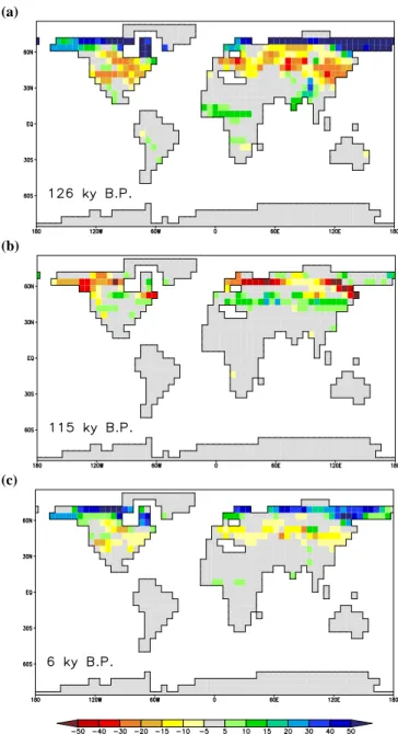
Fig. 2. Global distribution of biomes as calculated from LPJ, for (a) 126 ky B.P. (EEM), (b) 115 ky B.P. (EEM), (c) 6 ky B.P. (HOL), and (d) present (CTL). All plots show an average over 1000 years around the indicated time (present is an average over the complete CTL experiment, 10 000 years), for description of the biome calculation, see text and Table 1.

larger. The western part of the Sahara is covered with tem-perate grassland in the simulation, tropical forests in northern Africa and south Asia expand, and the boreal forests expand northward up to the Arctic Ocean in many places. In the southern hemisphere a slight retreat of forests is simulated for Africa. For 115 ky B.P. (Fig. 2b), the opposite is simu-lated: boreal forests in the northern hemisphere show a clear southward retreat and the vegetation cover in the monsoon areas decreases slightly, in most other regions vegetation pat-terns are very similar to simulated present-day conditions. 3.2.2 Comparison with vegetation reconstructions

Global data sets of paleovegetation are rare, and exist only for selected time slices. Few observations exist for the Eemian, because of a general lack of sites and difficulty with dating. For the Mid-Holocene data availability is much bet-ter.

Grichuk (1992) provides a reconstruction of northern hemisphere vegetation at the Eemian optimum. In the high latitudes it shows a decreased tundra area, coniferous forests

expand northward up to the Arctic Ocean. Some tundra areas remain in northeast Asia and the northeastern part of North America. This is consistent with the simulated distribution of tundra from the Eemian experiment (Fig. 2a). The forest zone shifts northward, especially for North America. In the simulation, the border between temperate and boreal forest is too far south compared to the reconstruction. The sub-tropical trees and bushes occupy a larger area: large parts of northern Africa are covered with savanna-type vegetation. This was found in the Eemian experiment as well, although the simulated extent is restricted to the western part of Africa (Fig. 2a).

A large set of Eemian pollen data for central Asia (Tarasov et al., 2005) reveals an increase of taiga till 125 ky B.P., fol-lowed by a period with relatively high boreal forest cover. At the end of the interglacial, temperate grassland and tundra become more dominant again.

Two nearly-global vegetation reconstructions were pre-sented by Prentice et al. (2000) for roughly 6 ky B.P. (based on pollen) and by Adams and Faure (1997) for roughly 8

114 116 118 120 122 124 126 128 250 260 270 280 290 300 p CO 2 (ppm) 0 2 4 6 8 250 260 270 280 290 300

Vostok ice core Taylor Dome ice core coupled experiment 114 116 118 120 122 124 126 128 -200 -100 0 100 200 300

terr. carbon anomaly (Pg C)

hyd rad 0 2 4 6 8 -200 -100 0 100 200 300 co2 tem Holocene Eemian time (ky B.P.) (a) (b) Partial experiments

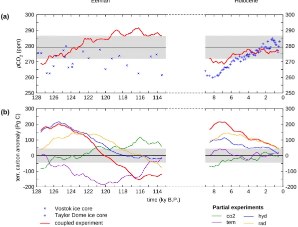
Fig. 3. Time series of (a) atmospheric CO₂concentration for the HOL and EEM experiment, with average of the CTL experiments, and (b) total carbon storage anomaly in the terrestrial biosphere for all experiments. Shown are 1000 year running means, the grey areas indicate ± 2 standard deviations of the CTL experiment. Vostok ice core CO₂concentration (Eemian, Petit et al., 1999) and Taylor Dome ice core CO₂ concentration (Holocene, Inderm¨uhle et al., 1999) are shown.

and 5 ky B.P. (based on fossils, pollen and other sources). Detailed comparison studies between data sets and model output were performed for the Mid-Holocene (6 ky B.P.) on a global scale (Harrison and Prentice, 2003) as well as in more detail for 55◦–90◦N (Kaplan et al., 2003). For 6000 year B.P., Hoelzmann et al. (1998) provided reconstructions for northern Africa as boundary conditions for modelling ex-periments, indicating that roughly the northern half of north Africa was mainly covered with grasslands, and the southern half was mainly covered with savanna. The main features of vegetation changes in these studies were obtained in the sim-ulation as well: a southward retreat of the border between boreal and temperate forest, and a decrease of vegetation in monsoon areas.

3.3 Terrestrial carbon storage

The simulated atmospheric CO2concentration increases

dur-ing both the Eemian and the Holocene experiment (Fig. 3a), starting around 270 ppm. For the Eemian experiment, a CO2 concentration of 280 ppm (which corresponds to the

pre-industrial level) is reached around 123 ky B.P., for the

Holocene experiment the CO2 concentration at the end

(0 ky B.P.) is 277 ppm. Interannual variability is remarkably large for the CTL experiment, the standard deviation of the 1000-year running means is 3.6 ppm.

For both interglacials, atmospheric CO2concentration and

terrestrial carbon storage show an opposite tendency, with an increase in atmospheric CO2content of about 40 Pg C

(cor-responding to 20 ppm CO2) for the Eemian and 20 Pg C

(cor-responding to 10 ppm CO2) for the Holocene, and a decrease

of the terrestrial carbon storage of about 350 Pg C for the Eemian and 200 Pg C for the Holocene (Fig. 3). The increase in CO2concentration is the result of this release of terrestrial

carbon (Fig. 3b), the remaining carbon released from the ter-restrial biosphere is taken up by the ocean. The decrease of terrestrial carbon storage is simulated for both the Eemian and the Holocene with trends of −37 Tg C yr−1(Eemian) and

−31 Tg C yr−1(Holocene), and with rather similar maxima (around 205 Pg C and 215 Pg C for 125 ky B.P. and 7 ky B.P., compared to the control simulation). After 120 ky B.P., ter-restrial carbon storage is smaller than in the control simula-tion, with a minimum of −150 Pg C for 116 ky B.P.

The spatial pattern for carbon storage shows that parti-cular regions play a dominant role in the changes during the interglacials (Fig. 4): The high latitudes north of 60◦_N

show a positive anomaly for 126 ky B.P. and 6 ky B.P. com-pared to the control simulation, for 115 ky B.P. this latitude band shows a negative anomaly. The mid-latitudes, between 30◦N and 60◦N, show the opposite signal: a negative carbon storage anomaly for 126 ky B.P. and 6 ky B.P., and a positive anomaly for 115 ky B.P. The monsoon regions in northern Africa and south Asia show a clear increase for 126 ky B.P., and a small effect for 6 ky B.P. as well. The southern hemi-sphere shows some small changes, but no clear pattern can be observed here.

Carbon storage anomalies for the Eemian and the Holocene can not be explained from a single climate para-meter (Fig. 3). All parapara-meters analysed here (temperature, radiation, hydrology and CO2) show effects on the total

car-bon storage that are larger than two standard deviations of the control state. These parameters were analysed in detail, and are discussed below.

The evolution of zonally integrated terrestrial carbon stor-age in time (Fig. 5a) shows the main features from the global distribution for selected periods in Fig. 4. The bands of in-creased and dein-creased storage in the high latitudes show a re-markable swap around 120 ky B.P. From 128 to 120 ky B.P., an increase was simulated for 60◦_–75◦_{N, a decrease for 40}◦_–

60◦_{N, and again an increase for 0}◦_–30◦_{N. After 120 ky B.P.}

the pattern shifts: a decrease was simulated for 55◦_–65◦_N,

and an increase is seen for 45◦–55◦N. 3.3.1 Temperature

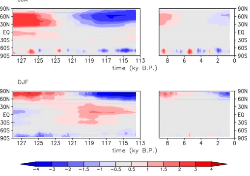
Temperature changes during the interglacials (Fig. 6) are a direct effect of changes in the earth’s orbit. Due to a sum-mer perihelion at 127 ky B.P., combined with a large eccen-tricity of the earth orbit, summer insolation for the northern hemisphere is enhanced compared to present-day for the first half of the Eemian experiment. This causes positive temper-ature anomalies in summer (Fig. 6). For the second half of the Eemian experiment, the perihelion occurs in winter for 116 ky B.P., causing a relatively low incoming radiation in summer, and an increase in insolation in winter (Fig. 6). For the Holocene, the effect is slightly less: although perihelion occurs in summer as well, the eccentricity is roughly half of the Eemian eccentricity, thereby reducing the differences be-tween summer and winter (Berger, 1978).

For the beginning of both Eemian and Holocene, the Northern Hemisphere summer is warmer, with a larger anomaly for the Eemian than for the Holocene. In the Eemian, warming occurs as well around the equator, while the monsoon areas of the Northern Hemisphere are rela-tively cooler due to increased evaporation and cloud cover, related to an enhancement of the monsoon precipitation. In the Eemian, a cooling up to 4 K occurs after 120 ky B.P. for the Northern Hemisphere north of 20◦N. A slight cooling

(a)

(b)

(c)

Fig. 4. Total terrestrial carbon storage anomalies (kg C m−2) for selected periods from the interglacial experiments: (a) 126 ky B.P. (EEM), (b) 115 ky B.P. (EEM), and (c) 6 ky B.P. (HOL). Anomalies from the control simulation (CTL) are shown for 2000 year periods around the given time.

(up to 1.5 K) was simulated for the last 2000 years of the Holocene as well, which is remarkable, and which shows that a steady-state control simulation does not necessarily provide the state that would be reached at the end of a tran-sient run. In the Northern Hemisphere winter, the latitudes north of 60◦N show a clear positive temperature anomaly at the beginning of both experiments. This positive anomaly changes to a negative anomaly after 120 ky B.P. A similar

(a)

(b)

(c)

(d)

(e)

Fig. 5. Zonal anomalies of total carbon storage per latitude (Pg C per degree latitude) for the Eemian and the Holocene with full climate forcing (a), as well as for the temperature only (b), hydrology only (c), radiation only (d) and CO2only (e) experiments.

pattern was simulated for the Holocene, although the mag-nitude is slightly smaller. Again a cooling was simulated for the last 2000 years of the Holocene. The tropics and subtropics show a clear warming for winters between 122 and 114 ky B.P. compared to the control run. In the Southern

Ocean, variability is high, and positive and negative temper-ature anomalies for summer and winter are mainly related to changes in the convection.

Temperature-induced changes in terrestrial carbon storage show the most prominent signal of all climate parameters for

Fig. 6. Zonal mean temperature anomalies for Northern Hemisphere summer (JJA) and winter (DJF) for the insolation experiments (EEM and HOL). Shown are 1000 year running means.

the mid- and high latitudes in the partial experiments (Fig. 5). For the beginning of the Eemian and Holocene experiments, an increased storage of carbon is simulated in the latitudes north of 60◦N compared to the present-day situation, and a decreased storage is simulated between 40◦N and 60◦N. The anomalies become smaller with time, and for the Eemian the decrease in the high latitudes and the increase in the mid latitudes continues after 119 ky B.P., resulting in opposite anomalies: the high latitudes have a decreased storage and the mid-latitudes an increased storage compared to present-day. Despite the large anomalies, the net effect on carbon storage is rather small and even negative for the Eemian ex-periment (Fig. 3b).

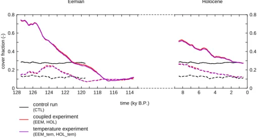
For the area north of 60◦N, temperature increase causes the region to become more favourable for forest growth; grasses and bare soil are there replaced by trees. Between 128 and 121 ky B.P., boreal forests cover a larger area than in the control simulation (Fig. 7). In the beginning of the exper-iment, cover is over 70% of the land surface north of 60◦N. After 125 ky B.P., forest cover declines sharply, and is parti-ally replaced by grass cover. A decline of both boreal trees and grasses causes the covers to become lower than in the control simulation around 121 ky B.P., with a minimum for-est cover of about 10% (around 117 ky B.P.). In the Holocene simulation, a decrease of forest fraction is simulated as well, although the maximum is not as high as for the Eemian. The increase in grass cover after retreat of the boreal forests is not seen in the Holocene, and the covers of both trees and grasses are roughly equal to the control values at the end of the Holocene experiment.

In the experiments forced with temperature of the coupled experiments only (EEM tem and HOL tem) the covers of bo-real forests and grasses have a very similar behaviour for the area north of 60◦N (Fig. 7), indicating that temperature is the main driver for the changes in cover fractions. These changes cause the carbon storage effect north of 60◦N. The area between 30◦N and 60◦N does not show large changes in the cover fraction. The changes in carbon storage here com-pared to the control experiment are related to changes in au-totrophic and heterotrophic respiration. Higher temperatures lead to higher respiration rates, which causes a reduction of the residence time of carbon. This effect is particularly ef-fective in reducing the size of soil carbon pools.

3.3.2 Hydrology

Climate change caused by variations in orbital forcing in-cludes changes in the hydrological cycle. Due to increased temperatures on land a stronger temperature gradient be-tween the land surface and the ocean occurs and monsoon circulation is strengthened, bringing more moist air to the continents and causing more convection. This results in an increase of precipitation over land and a decrease over the ocean, especially in the tropics and subtropics (Fig. 8a). The precipitation increase over land is substantially amplified by the positive feedback between albedo and precipitation (e.g. Claussen, 1997; Braconnot et al., 1999), as was discussed in Schurgers (2006) for the Eemian experiment.

The most important changes in carbon storage due to changes in the hydrological cycle take place between 10◦N

114 116 118 120 122 124 126 128 0 0.2 0.4 0.6 0.8 cover fraction (-) control run (CTL) coupled experiment (EEM, HOL) temperature experiment (EEM_tem, HOL_tem) 0 2 4 6 8 0 0.2 0.4 0.6 0.8 Holocene Eemian time (ky B.P.)

Fig. 7. Fractions of the land area between 60◦N and 90◦N covered with boreal trees (full line) and grasses (dashed line), for the control experiment (CTL), the coupled experiments (EEM and HOL) and the experiments forced with temperature only (EEM tem and HOL tem). Shown are 1000 year running means.

and 40◦N (Fig. 5c), where water availability is the main lim-iting factor for plant growth. Although local changes in car-bon storage are smaller than the changes caused by temper-ature in the higher latitudes, the latitude band being influ-enced is rather large, and the changes in the hydrological cycle cause a spatially constant positive effect on global car-bon storage between 128 and 121 ky B.P. and between 9 and 6 ky B.P. In contrast to temperature, there are no regional decreases in carbon storage due to hydrological changes for these periods, making hydrology one of the most important net effects of the anomalies seen for these periods in total carbon storage (Fig. 3b).

Figure 8a shows the positive anomaly of precipitation over the subtropical continents and the negative anomaly over the ocean between 128 and 121 ky B.P. and between 9 and 6 ky B.P. In northwest Africa, precipitation increased up to 500 mm per year compared to the pre-industrial control sim-ulation. A strong increase of precipitation occurred as well in the south Asian monsoon area around India, and at the west coast of North America. The most pronounced decrease of precipitation is found over the Atlantic Ocean, and to a lesser extent over the tropical Pacific. After 118 ky B.P., the north African as well as the North American subtropical and trop-ical parts of the continent become drier than the control sim-ulation.

Vegetation growth reacted strongly to the changes in pre-cipitation for most regions. The most sensitive regions are northwest Africa, south Asia around India, and western North America, with in general strong positive anomalies in vegetation cover between 128 and 121 ky B.P. and 9 and 6 ky B.P., and smaller negative anomalies from 118 ky B.P. onwards (Fig. 8b). Especially in northwest Africa and south

Asia, vegetation cover was higher than present-day at the beginning of both experiments. The Eemian shows a grad-ual decrease in vegetation cover in the western Sahara from about 40% to practically 0% from 124 ky B.P. to 118 ky B.P. (Schurgers, 2006). For the Holocene, maximum vegetation cover is roughly half of the Eemian cover, with a decrease from 9 ky B.P. to 4 ky B.P.

The increase in vegetation cover, as well as the conversion of grass-covered areas into forests, causes an increase in car-bon storage for northwest Africa and south Asia (Fig. 8c). The patterns of carbon storage are very similar to those shown for vegetation cover, with again stronger anomalies for the Eemian than for the Holocene simulation. The max-imum increase in global carbon storage due to hydrological changes (from the EEM hyd and HOL hyd experiments) was roughly twice as large for the Eemian than for the Holocene (Fig. 3b). This difference is directly related to the strength of the monsoon, which is mainly determined by the contrast in heating between the ocean and the land surface. Due to a decrease of surface albedo, this contrast is enhanced. This enhancement is larger for the Eemian than for the Holocene, because of the more eccentric earth orbit in the Eemian. In addition, the positive feedback between presence of vegeta-tion and precipitavegeta-tion enhances this contrast (see Schurgers, 2006, for a more detailed analysis).

3.3.3 Solar radiation

Solar radiation had for both the Eemian and the Holocene a direct positive influence on carbon storage for the latitudes between 45◦N and 70◦N during the warm phase (Fig. 5). The reason for this increase is an increase in photosynthe-sis in these latitudes, caused by an increase in absorbed

Fig. 8. Meridional anomalies of (a) precipitation (mm y−1) from the fully coupled experiments (EEM and HOL), and (b) vegetation cover (–) and (c) carbon storage (kg m−2) on land from the experiments with hydrological forcing only (EEM hyd and HOL hyd), all shown for the region 6◦–34◦N (see figure).

shortwave radiation. The radiation anomaly in these latitudes (Fig. 9) shows an increase of incoming radiation for the sum-mer months and the largest decrease for spring at the begin-ning of the experiment. Both the positive and the negative anomaly shift to earlier occurrence in the year, which causes the amplitude in the annual cycle of incoming radiation to be-come smaller, and both anomalies weaken during the

exper-iments. The incoming radiation at the surface shows a sim-ilar pattern as the incoming radiation at the top of the atmo-sphere, but with a smaller amplitude (not shown), due to ab-sorption of radiation in the atmosphere. Maximum increase in incoming radiation at the surface is around 40 W m−2_for

summer around 127 ky B.P., maximum decrease is around

at the surface is roughly 30 to 50% of the amplitude at the top of the atmosphere.

The influence of the changes in radiation on photosynthe-sis is shown in Fig. 10a. From 127 ky B.P. onwards, the maximum rate of photosynthesis decreased, and the peak in photosynthesis shifted to later in summer. Anomalies of gross primary production (GPP) compared to the control ex-periment (Fig. 10b) are a result of radiation and tempera-ture changes (Figs. 10c and d). The positive temperatempera-ture anomaly both in summer and in winter for the beginning of the Eemian experiment (Fig. 6) causes the growth and de-velopment of the vegetation to start earlier in the season, re-sulting in an increase of radiation absorption due to a faster leaf development and thereby in an increase of photosynthe-sis, especially in the first two months of the growing season (Fig. 10d). This effect is enhanced by a positive radiation anomaly for the summer months (Fig. 9), which results in additional photosynthesis (Fig. 10c). After 122 ky B.P. the temperature anomaly became negative for the region north of 60◦N, and the development of vegetation in spring becomes slower than in the control simulation. Due to the high radia-tion anomaly, the EEM rad experiment initially had a slightly positive anomaly in GPP later in the season for 121 ky B.P. (Fig. 10c), but this effect declines to zero as the radiation anomaly decreased.

3.3.4 CO2

Total terrestrial carbon storage in the experiments with CO2

as the varying forcing most clearly shows a first-order re-action to the atmospheric CO2 concentration (Fig. 3). In

these experiments, the amplitude of global net primary production (NPP) is roughly 4.5 Pg C y−1 (EEM co2) and 2 Pg C y−1(HOL co2), compared to a standard deviation of 1.7 Pg C y−1_{for the control simulation (CTL). These changes}

are small compared to changes from other factors, and are opposite in magnitude to the CO2signal of the coupled

ex-periments (Fig. 11), which demonstrates that the terrestrial biosphere is the driver of the changes in atmospheric CO2.

The effect of changes in the atmospheric CO2

concentra-tion are small on primary producconcentra-tion and small on carbon storage, which was to be expected because the terrestrial bio-sphere was the driver of these atmospheric CO2changes. A

terrestrial biosphere more sensitive to these changes than the one presented here would inevitably have led to a smaller signal in the atmospheric CO2concentration.

Ocean carbon storage rises throughout the Eemian and the Holocene. Most important is the increase of dissolved CO2 in the water column, as a reaction to the rising

atmo-spheric CO2 concentration. The sediment pool increases

initially for both the Eemian and the Holocene, reaching a positive anomaly of about 90 Pg C compared to the control run. From 124 ky B.P. and 7 ky B.P. onwards, sediment car-bon decreases due to a slight acidification of the ocean re-sulting from the uptake of atmospheric CO2, reaching a

neg-ative anomaly of 60 Pg C for the Eemian around 114 ky B.P. A detailed analysis of the Eemian carbon cycle is provided by Gr¨oger et al. (2006)1.

4 Discussion and conclusions

A complex earth system model was used to study terrestrial carbon storage during two interglacials, the Holocene and the Eemian. Under pre-industrial conditions, the model yields a reasonable distribution of the major vegetation zones, with some remarkable exceptions. In the Amazon region, large areas are covered with savanna type vegetation, because the simulated climate is too dry. The border between temperate and boreal forests was situated too far south, due to colder than observed temperatures in the Northern Hemisphere mid and high latitudes.

For the beginning of the Eemian and Holocene simula-tions, enhanced vegetation growth in north Africa and Asia around India caused a decrease of the desert area and an in-crease in savanna and temperate grassland. This is in agree-ment with reconstructions based on proxy data (e.g. Prentice et al., 2000). Forest cover in the high latitudes of the north-ern hemisphere decreased during both experiments due to a gradual cooling. This causes a southward retreat of the tree-line, which agrees with reconstructions (Adams and Faure, 1997; Prentice et al., 2000).

The changes in the distribution of vegetation, together with changes in photosynthesis rates, and changes in climate, cause changes in the storage of carbon in the terrestrial bio-sphere. These were the main cause for a gradual increase of the atmospheric CO2concentration during both interglacial

experiments. For both the Eemian and the Holocene, ter-restrial carbon storage was high in the beginning of the experiments, and gradually decreased from 125 ky B.P. and 8 ky B.P. onwards. These changes can be explained by the following relations between climate and the terrestrial car-bon cycle.

Temperature had the dominant effect on carbon storage, but its global net effect was small: the increase in sum-mer temperature of the mid and high latitudes around both 125 ky B.P. and 9 ky B.P. compared to the control simulation caused an increase in forest growth and photosynthesis and a corresponding increase in carbon storage for the high lati-tudes. Autotrophic and heterotrophic respiration increased as well due to the temperature increase, which in turn decreased carbon storage for the mid latitudes. Overall, these two op-posing processes caused the global temperature effect on ter-restrial carbon storage to be small in the coupled experiments that were performed here. With time, the anomalies become

1_{Gr¨oger, M., Maier-Reimer, E., Mikolajewicz, U., Schurgers,}

G., Vizca´ıno, M., and Winguth, A.: Changes in the hydrological cycle, ocean circulation and carbon/nutrient cycling during the last interglacial, Paleoceanography, submitted, 2006.

Fig. 9. Anomaly of the annual cycle of incoming shortwave radiation (W m−2) at the top of the atmosphere for 60◦N for the Eemian and Holocene. 1 2 3 4 5 6 7 8 9 10 11 12 month 0 100 200 300 400 500 GPP (g C m -2 month -1) CTL 127 ky B.P. 124 ky B.P. 121 ky B.P. 118 ky B.P. 115 ky B.P. 1 2 3 4 5 6 7 8 9 10 11 12 -200 -100 0 100 200 1 2 3 4 5 6 7 8 9 10 11 12 -200 -100 0 100 200 1 2 3 4 5 6 7 8 9 10 11 12 month -200 -100 0 100 200 EEM EEM_rad EEM_tem (b) (c) (d) (a)

Fig. 10. (a) Anual cycle of photosynthesis around 60◦N for selected periods (2000 year averages) from the Eemian coupled experiment (EEM) and the control experiment (CTL), and anomalies of the fully coupled experiment (b, EEM), the radiation only experiment (c, EEM rad), and the temperature only experiment (d, EEM tem), all compared to the control experiment (CTL).

smaller and in the Eemian experiment, the pattern swaps af-ter 120 ky B.P. compared to the control experiment. From the size of the positive and negative anomalies, it is clear that the net outcome is sensitive to changes in the sensitivity of both photosynthesis and autotrophic and heterotrophic respiration to temperature.

Changes in the hydrological cycle were a main cause for increased carbon storage in the subtropics. The region be-tween 10◦N and 40◦N had increased carbon storage com-pared to the control run from 128 to 121 ky B.P. and from 9 to 6 ky B.P. Although the local changes were much smaller

than those caused by temperature effects, they caused a posi-tive carbon storage anomaly for all regions for the beginning of the experiment. The globally averaged maximum storage increase due to hydrological changes was around 200 Pg C for the Eemian and around 100 Pg C for the Holocene. Solar radiation changes were also responsible for part of the in-creased carbon storage. Due to higher insolation in summer compared to the control simulation, photosynthesis increased for the land surface between 40◦ and 70◦N between 128 and 119 ky B.P., resulting in more carbon storage. Maximum anomalies due to radiation changes were roughly 150 Pg C

114 116 118 120 122 124 126 128 70 75 80 85 NPP (Pg C y -1 ) control run (CTL) coupled experiment (EEM, HOL) CO₂ experiment (EEM_co2, HOL_co2) 0 2 4 6 8 70 75 80 85 Holocene Eemian time (ky B.P.)

Fig. 11. Global net primary production (NPP) for the control experiment (CTL), the coupled experiments (EEM and HOL) and the experi-ments forced with CO2only (EEM co2 and HOL co2). Shown are 1000 year running means.

for both the Eemian and the Holocene. Changing CO2

con-centration had a minor influence on the terrestrial carbon storage.

From a previous study with the same earth system model (Mikolajewicz et al., 2006), the distribution of CO2

emit-ted over atmosphere, land and ocean equilibraemit-ted at approxi-mately 10%, 18% and 72%, using a scenario with relatively low emissions. In the insolation experiments presented here, the ratio between marine and atmospheric storage is higher than for this equilibrium state, especially for the beginning of both experiments, when marine storage is lower than the con-trol run. This deviation from the equilibrium state could be caused by the gradual CO2change, which inhibits especially

the ocean from reaching equilibrium, and by changes in cli-mate, which could cause that the ocean is not just playing a passive role in the interglacial carbon cycle.

The effect of the increasing atmospheric CO2

concentra-tion on climate is expected to be minor: the increase of 20 ppm (Eemian) and 10 ppm (Holocene) would lead to an increase of about 0.1 to 0.2 K, assuming the system would be able to equilibrate. The temperature sensitivity of the earth system model to a doubling of the CO2concentration is 2.3 K

after equilibration (Mikolajewicz et al., 2006).

The changes in CO2concentration are both for terrestrial

carbon storage and for global climate minor effects. Despite the rising concentration, both global temperature (Fig. 1a) and terrestrial carbon storage (Fig. 3b) decrease during the interglacials. Terrestrial carbon storage was a main driver of the changes in atmospheric CO2. This indicates that the

neg-ative feedback between terrestrial carbon storage and CO2

concentration is rather weak, as well as the feedback between CO2 concentration and climate change. The changes in the

orbital forcing are of much larger importance for both carbon storage and climate.

An estimate of terrestrial carbon storage for the Holocene at 8 ky B.P., based on a reconstructions of the vegetation dis-tribution combined with estimates of carbon storage in se-lected ecosystems was derived by Adams and Faure (1998). They calculate a negative anomaly of terrestrial carbon stor-age compared to present-day of 170 Pg C. Somewhat smaller estimates are simulated with the LPJ model by Kaplan et al. (2002) and Joos et al. (2004): both show an increase in ter-restrial carbon storage for the Holocene from the last glacial maximum onwards, with a small increase (∼100 Pg C) dur-ing the last 8000 years. Oceanic release of carbon is sup-posed to be responsible for the increasing atmospheric CO2

concentration in these studies.

In this study we observed the opposite effect: for the last 8000 years it showed a decrease in terrestrial carbon stor-age of 200 Pg C. This is in agreement with the estimate by Inderm¨uhle et al. (1999) of 260 Pg C for 7–1 ky B.P. A de-crease was simulated by Brovkin et al. (2002) as well, with a magnitude of 90 Pg C for 8 ky B.P.–present. The simulated atmospheric CO2concentration showed similar trends for the

Eemian and the Holocene. The amplitude of CO2changes

for the Holocene is too small compared to ice core measure-ments (Inderm¨uhle et al., 1999). For the Eemian, the com-parison between model and data is harder, because there are less data points, and there is no clear trend in the data. Dif-ferences between the terrestrial carbon and atmospheric CO2

estimates, as well as uncertainties about the terrestrial bio-sphere being a source or a sink of carbon during the last 8000 years, could be due to uncertainties in the temperature ef-fect. The simulations showed that temperature changes have two opposing effects, of which the net outcome might be climate- and model-dependent. A second important factor for the difference between model results and observations is related to the initial conditions. The steady-state present-day

circulation that was used here to start the simulations from does not reflect the actual transition from the glacial that pre-ceded the interglacials. Besides that, Kaplan et al. (2002) state that they might have underestimated the carbon loss due to changes in the monsoon. In our simulations, changes in the hydrological cycle were responsible for a decrease of 100 Pg C during the last 8000 years.

The effect of peat buildup during interglacials was not taken into account in the model simulations presented here. Global estimates of uptake of atmospheric CO2are between

180 and 450 Pg C from the Last Glacial Maximum onwards, with most of it taken up during the last 9000 years (Gajewski et al., 2001; Smith et al., 2004). This is a potentially impor-tant sink of CO2, although it would replace the currently

sim-ulated boreal forests and grasslands. As the density of soil carbon is high in the high latitudes anyway, the net change might be relatively small.

For a better representation of the terrestrial biosphere and the carbon cycle therein, dynamic simulation of peatlands should be included, as well as a better description of soil carbon processes and soil formation. The use of dynamic ice sheets would provide more reliable initial conditions, and would allow for extending the simulations into the glacial pe-riods. These factors are causing uncertainties in the outcome of this study, and should be addressed for future studies on interglacial climate and carbon cycle.

In the simulations presented here, changes in the CO2

con-centration for the interglacials were shown to be caused by changes in terrestrial carbon storage. However, this is not at all indicative for carbon storage during glacials, or for interglacial-to-glacial transitions. During glacials, terrestrial carbon storage is hypothesized to have been low because of low temperatures and a weak hydrological cycle. An ex-planation for the low CO2 concentrations observed during

glacial periods (Petit et al., 1999) cannot be found in the mechanisms described here.

Acknowledgements. This study was performed within the

CLIM-CYC project, funded by the DEKLIM program of the German Ministry of Education and Research (BMBF). The simulations were performed at the German Climate Computing Centre (DKRZ). We thank M. Claussen as well as V. Brovkin and J. Kaplan for helpful remarks.

Edited by: N. Weber

References

Adams, J. and Faure, H.: Preliminary vegetation maps of the world since the last glacial maximum: an aid to archaeological under-standing, J. Archaeol. Sci., 24, 623–647, 1997.

Adams, J. and Faure, H.: A new estimate of changing carbon stor-age on land since the last glacial maximum, based on global land ecosystem reconstruction, Global Planet. Change, 16–17, 3–24, 1998.

Berger, A.: Long-term variations of daily insolation and Quaternary climate changes, J. Atmos. Sci., 35, 2362–2367, 1978.

Braconnot, P., Joussaume, S., Marti, O., and de Noblet, N.: Syner-gistic feedbacks from ocean and vegetation on the African mon-soon response to mid-Holocene insolation, Geophys. Res. Lett., 26, 2481–2484, 1999.

Broecker, W. and Clark, E.: Holocene atmospheric CO2increase as

viewed from the seafloor, Global Biogeochem. Cycles, 17, 1052, doi:10.1029/2002GB001985, 2003.

Brovkin, V., Bendtsen, J., Claussen, M., Ganopolski, A., Kubatzki, C., Petoukhov, V., and Andreev, A.: Carbon cycle, vegeta-tion, and climate dynamics in the Holocene: Experiments with the CLIMBER-2 model, Global Biogeochem. Cycles, 16, 1139, doi:10.1029/2001GB001662, 2002.

Claussen, M.: Modelling bio-geophysical feedback in the African and Indian monsoon region, Clim. Dyn., 13, 247–257, 1997. Gajewski, K., Viau, A., Sawada, M., Atkinson, D., and Wilson, S.:

Sphagnum peatland distribution in North America and Eurasia during the past 21,000 years, Global Biogeochem. Cycles, 15, 297–310, 2001.

Grichuk, V.: Vegetation during the last interglacial, in: Atlas of pa-leoclimates and paleoenvironments of the Northern Hemisphere, edited by: Frenzel, B., P´ecsi, M., and Velichko, A., Gustav Fis-cher Verlag, Stuttgart, 1992.

Harrison, S. and Prentice, C.: Climate and CO2controls on global

vegetation distribution at the Last Glacial Maximum: analysis based on paleovegetation data, biome modelling and paleocli-mate simulations, Global Change Biol., 9, 983–1004, 2003. Hoelzmann, P., Jolly, D., Harrison, S., Laarif, F., Bonnefille, R., and

Pachur, H.-J.: Mid-Holocene land-surface conditions in northern Africa and the Arabian peninsula: A data set for the analysis of biogephysical feedbacks in the climate system, Global Bio-geochem. Cycles, 12, 35–51, 1998.

Inderm¨uhle, A., Stocker, T., Joos, F., Fischer, H., Smith, H., Wahlen, M., Deck, B., Mastroianni, D., Tschumi, J., Blunier, T., Meyer, R., and Stauffer, B.: Holocene carbon-cycle dynamics based on CO2trapped in ice at Taylor Dome, Antarctica, Nature,

398, 121–126, 1999.

Joos, F., Gerber, S., Prentice, I., Otto-Bliesner, B., and Valdes, P.: Transient simulations of Holocene atmospheric carbon dioxide and terrestrial carbon since the Last Glacial Maximum, Global Biogeochem. Cycles, 18, GB2002, doi:10.1029/2003GB002156, 2004.

Kaplan, J., Prentice, I., Knorr, W., and Valdes, P.: Mod-eling the dynamics of terrestrial carbon storage since the Last Glacial Maximum, Geophys. Res. Lett., 29, 2074, doi:10.1029/2002GL015230, 2002.

Kaplan, J., Bigelow, N., Prentice, I., Harisson, S., Bartlein, P., Christensen, T., Cramer, W., Matveyeva, N., McGuire, A., Mur-ray, D., Razzhivin, V., Smith, B., Walker, D., Anderson, P., An-dreev, A., Brubaker, L., Edwards, M., and Lozhkin, A.: Cli-mate change and Arctic ecosystems: 2. Modelling, paleodata-model comparisons, and future projections, J. Geophys. Res., 108, 8171, doi:10.1029/2002JD002559, 2003.

Maier-Reimer, E.: Geochemical cycles in an ocean general cir-culation model. Preindustrial tracer distributions, Global Bio-geochem. Cycles, 7, 645–677, 1993.

Mikolajewicz, U., Scholze, M., and Voss, R.: Simulating near-equilibrium climate and vegetation for 6000 cal. years BP., The

Holocene, 13, 319–326, 2003.

Mikolajewicz, U., Gr¨oger, M., Maier-Reimer, E., Schurgers, G., Vizca´ıno, M., and Winguth, A.: Long-term effects of anthro-pogenic CO2emissions simulated with a complex earth system

model, Clim. Dyn., in press, doi:10.1007/s00382-006-0204-y, 2006.

Petit, J., Jouzel, J., Raynaud, D., Barkov, N., Barnola, J.-M., Basile, I., Bender, M., Chappelaz, J., Davis, M., Delaygue, G., Delmotte, M., Kotlyakov, V., Legrand, M., Lipenkov, V., Lorius, C., P´epin, L., Ritz, C., Saltzman, E., and Stievenard, M.: Climate and at-mospheric history of the past 420,000 years from the Vostok ice core, Antarctica, Nature, 399, 429–436, 1999.

Prentice, I. and Webb III, T.: BIOME 6000: reconstructing global mid-Holocene vegetation patterns from palaeoecological records, J. Biogeogr., 25, 997–1005, 1998.

Prentice, I., Jolly, D., and BIOME 6000 participants: Mid-Holocene and glacial-maximum vegetation geography of the northern con-tinents and Africa, J. Biogeogr., 27, 507–519, 2000.

Ruddiman, W.: The anthropogenic greenhouse era began thousands of years ago, Clim. Change, 61, 261–293, 2003.

Sausen, R. and Voss, R.: Techniques for asynchronous and peri-odically synchronous coupling of atmosphere and ocean models. Part I: general strategy and application to the cyclo-stationary case, Clim. Dyn., 12, 313–323, 1996.

Schurgers, G.: Long-term interactions between vegetation and cli-mate – Model simulations for past and future, Berichte zur Erdsystemforschung, 27, Hamburg, http://www.mpimet.mpg.de/ en/wissenschaft/publikationen/erdsystemforschung.html, 2006.

Sitch, S., Smith, B., Prentice, I., Arneth, A., Bondeau, A., Cramer, W., Kaplan, J., Levis, S., Lucht, W., Sykes, M., Thonicke, K., and Venevsky, S.: Evaluation of ecosystem dynamics, plant geogra-phy and terrestrial carbon cycling in the LPJ Dynamic Global Vegetation Model, Global Change Biol., 9, 161–185, 2003. Smith, L., MacDonald, G., Velichko, A., Beilman, D., Borisova,

O., Frey, K., Kremenetski, K., and Sheng, Y.: Siberian peat-lands a net carbon sink ang global methane source since the early Holocene, Science, 303, 353–356, 2004.

Tarasov, P., Granoszweski, W., Bezrukova, E., Brewer, S., Nita, M., Abzaeva, A., and Oberh¨ansli, H.: Quantitative reconstruction of the last interglacial vegetation and climate based on pollen record from Lake Baikal, Russia, Clim. Dyn., 25, 625–637, doi:10.1007/s00382-005-0045-0, 2005.

Voss, R. and Mikolajewicz, U.: Long-term climate changes due to increased CO2 concentration in the coupled atmosphere-ocean

general circulation model ECHAM3/LSG, Clim. Dyn., 17, 45– 60, 2001.

Winguth, A., Mikolajewicz, U., Gr¨oger, M., Maier-Reimer, E., Schurgers, G., and Vizca´ıno, M.: CO2uptake of the marine

bio-sphere: Feedbacks between the carbon cycle and climate change using a dynamic earth system model, Geophys. Res. Lett., 32, L23714, doi:10.1029/2005GL023681, 2005.