HAL Id: hal-03152249
https://hal.archives-ouvertes.fr/hal-03152249
Submitted on 27 Feb 2021
HAL is a multi-disciplinary open access
archive for the deposit and dissemination of
sci-entific research documents, whether they are
pub-lished or not. The documents may come from
teaching and research institutions in France or
abroad, or from public or private research centers.
L’archive ouverte pluridisciplinaire HAL, est
destinée au dépôt et à la diffusion de documents
scientifiques de niveau recherche, publiés ou non,
émanant des établissements d’enseignement et de
recherche français ou étrangers, des laboratoires
publics ou privés.
Carbon stars in the X-Shooter Spectral Library
A. Gonneau, A. Lançon, S. Trager, B. Aringer, M. Lyubenova, W. Nowotny,
R. Peletier, P. Prugniel, Y.-P. Chen, M. Dries, et al.
To cite this version:
A. Gonneau, A. Lançon, S. Trager, B. Aringer, M. Lyubenova, et al.. Carbon stars in the
X-Shooter Spectral Library. Astronomy and Astrophysics - A&A, EDP Sciences, 2016, 589, pp.A36.
�10.1051/0004-6361/201526292�. �hal-03152249�
A&A 589, A36 (2016) DOI:10.1051/0004-6361/201526292 c ESO 2016
Astronomy
&
Astrophysics
Carbon stars in the X-Shooter Spectral Library
?,??,???
A. Gonneau
1,2, A. Lançon
1, S. C. Trager
2, B. Aringer
3,4, M. Lyubenova
2, W. Nowotny
3, R. F. Peletier
2,
P. Prugniel
5, Y.-P. Chen
6, M. Dries
2, O. S. Choudhury
7, J. Falcón-Barroso
8,9, M. Koleva
10,
S. Meneses-Goytia
2, P. Sánchez-Blázquez
11,12, and A. Vazdekis
8,91 Observatoire Astronomique de Strasbourg, Université de Strasbourg, CNRS, UMR 7550, 11 rue de l’Université,
67000 Strasbourg, France
e-mail: anais.gonneau@astro.unistra.fr
2 Kapteyn Astronomical Institute, University of Groningen, Postbus 800, 9700 AV Groningen, The Netherlands 3 University of Vienna, Department of Astrophysics, Türkenschanzstraße 17, 1180 Wien, Austria
4 Dipartimento di Fisica e Astronomia Galileo Galilei, Università di Padova, Vicolo dell’Osservatorio 3, 35122 Padova, Italy 5 CRAL-Observatoire de Lyon, Université de Lyon, Lyon I, CNRS, UMR 5574, 69007 Lyon, France
6 New York University Abu Dhabi, PO Box 129188, Abu Dhabi, UAE
7 Leibniz-Institut für Astrophysik Potsdam (AIP), An der Sternwarte 16, 14482 Potsdam, Germany 8 Instituto de Astrofísica de Canarias, vía Láctea s/n, La Laguna, 38205 Tenerife, Spain
9 Departamento de Astrofísica, Universidad de La Laguna, 38205 La Laguna, Tenerife, Spain 10 Sterrenkundig Observatorium, Universiteit Gent, Krijgslaan 281, 9000 Gent, Belgium
11 Universidad Autónoma de Madrid, Departamento de Física Teórica, 28049 Cantoblanco, Madrid, Spain 12 Instituto de Astrofísica, Facultad de Fisica, Pontificia Universidad Catolica de Chile, Santiago 22, Chile
Received 9 April 2015/ Accepted 20 December 2015
ABSTRACT
We provide a new collection of spectra of 35 carbon stars obtained with the ESO/VLT X-Shooter instrument as part of the X-Shooter Spectral Library project. The spectra extend from 0.3 µm to 2.4 µm with a resolving power above ∼8000. The sample contains stars with a broad range of (J − K) color and pulsation properties located in the Milky Way and the Magellanic Clouds.
We show that the distribution of spectral properties of carbon stars at a given (J − K) color becomes bimodal (in our sample) when (J − K) is larger than about 1.5. We describe the two families of spectra that emerge, characterized by the presence or absence of the absorption feature at 1.53 µm, generally associated with HCN and C2H2. This feature appears essentially only in large-amplitude
va-riables, though not in all observations. Associated spectral signatures that we interpret as the result of veiling by circumstellar matter, indicate that the 1.53 µm feature might point to episodes of dust production in carbon-rich Miras.
Key words.stars: AGB and post-AGB – stars: carbon – infrared: stars – ultraviolet: stars
1. Introduction
In the 1860s, Father Angelo Secchi discovered a new type of star – Type IV – known today as carbon stars (Secchi 1868). Carbon stars (hereafter C stars) are on the asymptotic giant branch (AGB) and have spectra that differ dramatically from those of K- or M-type giants. C stars are characterized by spec-tral bands of carbon compounds, such as CN and C2bands, and
by the lack of bands from oxides such as TiO and H2O. The
clas-sical distinction between carbon-rich and oxygen-rich stars is the ratio of carbon to oxygen abundance, C/O. If C/O > 1, oxygen is mostly bound to carbon in the form of carbon monoxide (CO) because this molecule has a high binding energy. As a re-sult, little oxygen is left to form other oxides in these stellar ? Based on observations collected at the European Southern
Observatory, Paranal, Chile, Prog. ID 084.B-0869(A/B), 085.B-0751(A/B), 189.B-0925(A/B/C/D).
?? Tables1,B.1,E.1,E.2are also available at the CDS via
anonymous ftp tocdsarc.u-strasbg.fr(130.79.128.5) or via http://cdsarc.u-strasbg.fr/viz-bin/qcat?J/A+A/589/A36
???
The reduced spectra are only available at the CDS via anonymous ftp tocdsarc.u-strasbg.fr(130.79.128.5) or via
http://cdsarc.u-strasbg.fr/viz-bin/qcat?J/A+A/589/A36
atmospheres, whereas carbon atoms are available to form other carbon compounds.
Carbon stars are significant contributors to the near-infrared light of intermediate age stellar populations (1–3 Gyr) (e.g.,
Ferraro et al. 1995; Girardi & Bertelli 1998; Maraston 1998;
Lançon et al. 1999;Mouhcine & Lançon 2002;Maraston 2005;
Marigo & Girardi 2007). The absolute level of this contribution has an impact on mass-to-light ratios and has important implica-tions for the study of star formation in the Universe. It is a mat-ter of active research both on the theoretical side (e.g.,Weiss & Ferguson 2009;Girardi et al. 2013;Marigo et al. 2013) and in the framework of extragalactic observations (e.g.,Riffel et al. 2008;
Kriek et al. 2010; Miner et al. 2011; Melbourne et al. 2012;
Melbourne & Boyer 2013;Boyer et al. 2013;Zibetti et al. 2013). The quality of the photometric and spectroscopic predictions made by population synthesis models in this field depends on the existence of stellar spectral libraries, and their completeness in terms of evolutionary stages and spectral types.
Carbon stars contribute significantly to the chemical enrich-ment and to the infrared light of galaxies, but only small collec-tions of C-star spectra exist to represent this emission (seeLloyd Evans 2010, for a review that includes earlier observations). As a reference for C-star classification,Barnbaum et al.(1996)
published an extensive low-resolution optical spectral atlas (0.4–0.7 µm). It contains 119 spectra. Joyce(1998) provided a first impression of the near-infrared (NIR) spectra of C stars, again at low spectral resolution (48 spectra, with a spectral re-solution of ∼500). Repeated observations of single long-period variable (LPV) stars showed significant changes with phase, em-phasizing the necessity of simultaneous observations across the spectrum. As NIR detectors improved,Lançon & Wood(2000) produced a library of 0.5–2.5 µm spectra of luminous cool stars with a resolving power R= λ/∆λ ' 1100 in the NIR. It includes 25 spectra of seven carbon stars. Simultaneous optical spectra are available for 21 of them, but only at very low resolution (R ' 200). More recently,Rayner et al.(2009) have published the IRTF Spectral Library, which includes 13 stars of spectral type S (C/O = 1) or C. Their spectra have no optical counter-parts, but extend from 0.8 µm as far as 5.0 µm at a resolving power R ∼ 2000.
Several population synthesis models have used the C-star collection of Lançon & Wood (2000) (Lançon et al. 1999;
Mouhcine & Lançon 2002;Maraston 2005;Marigo et al. 2008).
Lançon & Mouhcine (2002) suggested using a near-infrared color as a first-order classification parameter for the C-star spectra in these applications, but also noted that this disre-gards other potentially important parameters, such as the carbon-to-oxygen (C/O) ratio or the pulsation properties. One of the shortcomings of this data set is the narrow range of properties (Lyubenova et al. 2010,2012). Another is that it simply contains too few stars to represent the variety of C-stars pectra.
In modeling of luminous cool stellar populations, two im-portant sources of uncertainties (other than the incompleteness of spectral libraries) are the fundamental parameters assigned to the observed stars and the effects of circumstellar dust related to pulsation and mass loss on the upper asymptotic giant branch. Estimating effective temperatures, C/O ratios, and gravities re-quires a comparison with theoretical spectra.Loidl et al.(2001) showed that it is difficult to obtain a good theoretical represen-tation of both the energy distribution and the spectral features, even for relatively blue C stars. Aringer et al. (2009) pointed out that static models without circumstellar dust cannot repro-duce any NIR carbon star energy distribution with (J − K) > 1.6.
Nowotny et al.(2011,2013) computed small numbers of spectral energy distributions for pulsating models, at low spectral resolu-tion. They reproduce the overall trend from optical carbon stars to dust-enshrouded sources, for which the whole spectrum is dominated by the emission from dust shells. But whether or not they reproduce the relationship between color and the depth of spectral features remains an open question. It is important to find out how dust shells may affect the optical and near-infrared spec-tra of C stars, especially for objects in the range 1.4 <∼ (J−K) <∼ 2 where the NIR luminosities of these AGB stars are large.
In this paper, we present spectra of 35 medium-resolution carbon stars extending from the near-ultraviolet through the op-tical into the near-infrared (0.3–2.5 µm). Although this collec-tion is by itself not complete, it considerably extends the range of data available, and it offers unprecedented spectral resolu-tion. We expect it to serve both the purpose of testing theoret-ical models for C-star spectra (Gonneau et al., in prep.) and of improving future population synthesis models. We describe the input stellar spectral library, our sample selection and the data reduction in Sects.2and3. We discuss the spectra using a NIR color as a primary classification criterion in Sect.4; in particular we discuss the appearance of a bimodal behavior of the spectral features and the overall spectral energy distribution in the red-der C-star spectra. We define a list of spectroscopic indices in
Sect.5that we use in Sect. 6to quantify the spectral behavior and in Sect.7 to compare our spectra with existing libraries of carbon-rich stars. We discuss our results in Sect.8and present our conclusions in Sect.9.
2. The XSL carbon star sample
With X-Shooter (Vernet et al. 2011), the European Southern Observatory (ESO) made available a high-throughput spectro-graph allowing the simultaneous acquisition of spectra from 0.3 to 2.5 µm, using two dichroics to split the beam into three wave-length ranges, referred to as arms: ultraviolet-blue (UVB), visi-ble (VIS) and near-infrared (NIR). This simultaneity is invalua-ble when observing variainvalua-ble stars, and many C stars are LPVs (Lloyd Evans 2010).
Our team is building a large stellar spectral library under an ESO Large Programme, the X-Shooter Spectral Library (here-after XSL,Chen et al. 2014). It contains more than 700 stars, observed at moderate resolving power (7700 ≤ R ≤ 11 000, depending on the arm) and covering a large range of stellar at-mospheric parameters. The homogeneous spectroscopic exten-sion into the near-infrared makes XSL unique among empirical libraries.
In this paper, we focus only on carbon stars. Table1 gives a full description of the C-star sample. TableB.1summarizes properties of these stars as available in the literature.
The sample includes stars from the Milky Way (MW) as well as from the Large and Small Magellanic Clouds (LMC, SMC). As C stars on the AGB form a relatively tight sequence in NIR color–color plots (2MASS,Skrutskie et al. 2006; DENIS,
Epchtein et al. 1997; WISE,Wright et al. 2010;Whitelock et al. 2006;Nowotny et al. 2011), the primary aim of the selection was to sample an adequate range of near-infrared colors. This range was restricted to (J − K) < 3 to avoid stars with negli-gible optical flux. A few C stars with (J − K) < 1 are present in the sample, although these stars are considered too hot to be standard AGB objects; they are instead thought to have become carbon-rich through other processes, such as mass transfer from a companion.
While the effects of metallicity on stellar evolution tracks are large, leading to varying estimates of the fraction of C stars as a function of metallicity (Mouhcine et al. 2002; Mouhcine & Lançon 2003; Marigo et al. 2008; Groenewegen 2007), the effects of initial metallicity on the spectrum of a C star of a given color are relatively small based on static models (Loidl et al. 2001; Gonneau et al., in prep). Therefore, we initially con-sider all stars in the sample as one group, irrespective of the host galaxy.
A variety of LPV pulsation amplitudes and light curve shapes can be found in C stars with 1 <∼ (J − K) <∼ 3. A distinct period and a clear period-luminosity relation exist for large-amplitude variables (e.g.,Whitelock et al. 2006), but many smaller-amplitude variables found in this range have extremely irregular light curves (seeHughes & Wood 1990). As shown in Figs.1and2, there are systematic differences between the pul-sation properties of our subsamples of C stars from the MW, the LMC and the SMC. On average, the LMC subset has a larger pulsation amplitude. More specifically, all the LMC stars in our sample display Mira-type pulsation, while the majority of the other stars in our sample are semi-regular variables, with com-paratively small amplitudes (TableB.1). In addition, at a given color, the SMC stars tend to be brighter than their LMC coun-terparts (no reliable distances are available for the MW stars of
Table 1. Observational properties of our sample.
Name Coordinates Host ESO ESO MJD Flux (J − Ks) Group 1.53 µm
(J2000) Period OBid notea [mag]b c featured
Cl* NGC 121 T V8 00:26:48.52 −71:32:50.5 SMC P89 723477 56 090.41 N 1.06 1 2MASS J00490032-7322238 00:49:00.33 −73:22:23.8 SMC P84 389528 55 110.07 N 1.50 2 2MASS J00493262-7317523 00:49:32.62 −73:17:52.3 SMC P84 389526 55 110.09 N 1.44 2 2MASS J00530765-7307477 00:53:07.65 −73:07:47.8 SMC P84 389511 55 116.12 N 1.43 2 2MASS J00542265-7301057 00:54:22.66 −73:01:05.7 SMC P84 389505 55 119.07 N 1.92 3 2MASS J00553091-7310186 00:55:30.91 −73:10:18.6 SMC P84 389503 55 119.09 N 2.11 3 2MASS J00563906-7304529 00:56:39.06 −73:04:53.0 SMC P84 389499 55 114.12 N 1.37 2 2MASS J00564478-7314347 00:56:44.78 −73:14:34.7 SMC P84 389497 55 119.11 N 1.77 3 2MASS J00570070-7307505 00:57:00.70 −73:07:50.6 SMC P84 389495 55 111.07 N 1.66 3 2MASS J00571214-7307045 00:57:12.15 −73:07:04.6 SMC P84 389493 55 111.08 N 1.53 2 2MASS J00571648-7310527 00:57:16.48 −73:10:52.8 SMC P84 389489 55 111.11 N 1.31 2 2MASS J01003150-7307237 01:00:31.51 −73:07:23.7 SMC P84 389481 55 111.12 N 1.33 2 Cl* NGC 419 LE 35 01:08:17.49 −72:53:01.3 SMC P90 804029 56 213.20 V 2.09 3 Cl* NGC 419 LE 27 01:08:20.67 −72:52:52.0 SMC P90 804024 56 213.18 V 1.98 3 T Cae 04:47:18.92 −36:12:33.5 MW P84 389 388 55 142.19 N/S 1.63 3 SHV 0500412-684054 05:00:29.71 −68:36:37.4 LMC P90 804254 56 213.29 1.84 3 Y SHV 0502469-692418 05:02:28.86 −69:20:09.7 LMC P90 804257 56 213.31 1.98 3 Y SHV 0504353-712622 05:03:55.96 −71:22:22.1 LMC P84 389445 55 119.26 N 2.17 3 SHV 0517337-725738 05:16:33.31 −72:54:32.1 LMC P90 804263 56 213.36 1.13 1 SHV 0518222-750327 05:16:49.73 −75:00:22.7 LMC P84 389433 55 142.28 N 2.52 4 Y SHV 0518161-683543 05:18:02.47 −68:32:39.1 LMC P90 804266 56 234.29 N 1.16 1 SHV 0520505-705019 05:20:15.02 −70:47:26.1 LMC P84 389428 55 142.32 N 2.37 4 Y SHV 0520427-693637 05:20:20.19 −69:33:44.8 LMC P90 804284 56 240.35 2.11 3 SHV 0528537-695119 05:28:27.73 −69:49:01.8 LMC P84 389414 55 226.19 V/ N 3.23 4 Y SHV 0525478-690944 05:25:28.21 −69:07:13.2 LMC P84 389421 55 142.36 N 3.02 4 Y SHV 0527072-701238 05:26:37.82 −70:10:11.6 LMC P90 804300 56 261.34 2.55 4 Y SHV 0536139-701604 05:35:42.81 −70:14:16.3 LMC P84 389406 55 226.23 N 3.12 4 Y [ABC89] Pup 42 08:04:57.56 −29:51:25.5 MW P90 804003 56 292.25 2.30 4 IRAS 09484-6242 09:49:49.40 −62:56:09.0 MW P92 998 138 56 617.34 2.02 3 [W65] c2 11:22:05.06 −59:38:45.2 MW P90 804 322 56 320.35 1.71 3 [ABC89] Cir 18 13:55:26.20 −59:22:19.0 MW P89 814763 56 319.37 2.45 4 MW P91 929 000 56383.31 2.52 4 HE 1428-1950 14:30:59.39 −20:03:41.9 MW P91 929514 56 383.33 0.71 1 V CrAc 18:47:32.31 −38:09:32.3 MW P89 723829 56 144.17 – – HD 202851 21:18:43.48 −01:32:03.3 MW P89 723822 56 144.31 N 0.83 1
Notes.(a)The letter indicates for which X-Shooter arm no absolute flux-calibration was possible: V=visible, N=near-infrared. The S letter indicates
that the spectrum is saturated in the K-band.(b)The (J − K
s) colors are derived from the spectra using the 2MASS filters (Cohen et al. 2003), see
Sect.5.1.(c)The group sharing is discussed in Sect.4.(d)The Y letter indicates the presence of the 1.53 µm absorption band (see Sect.4).(e)See
AppendixAfor more details about V CrA.
the sample). These selection biases must be kept in mind when interpreting the spectra, which is another reason to treat the com-bined samples as one sample.
3. Data reduction
In the following section, we summarize the applied data reduc-tion procedures. The carbon star data were acquired over ESO Periods 84, and 89 to 92 (Table1). The narrow-slit widths for UVB, VIS and NIR images were 0.500, 0.700, 0.600, respectively. 3.1. UVB and VIS arms: extraction and flux-calibration The UVB- and VIS-arm carbon star spectra observed in Period 84 are part of XSL Data Release I (DRI,Chen et al. 2014) and are used here unchanged. The basic data reduction for DRI was performed with X-Shooter pipeline version 1.5.0, up to the crea-tion of rectified, wavelength-calibrated two-dimensional (2D) spectra. The extraction of one-dimensional (1D) spectra was per-formed outside of the pipeline with a procedure inspired by the prescription ofHorne(1986). Observations of both the science targets and spectrophotometric standard stars through a wide
slit (5.0000) were used to obtain absolute fluxes (see Table1for
exceptions).
We reduced UVB and VIS spectra from later periods with X-Shooter pipeline version 2.2.0 (Modigliani et al. 2010). For the purposes of this paper, the pipeline was also used for the extraction of 1D spectra and flux calibration. The choice of pipeline version does not affect our conclusions.
3.2. NIR arm: extraction
All NIR images were reduced with X-Shooter pipeline ver-sion 2.2.0, up to the creation of rectified, wavelength-calibrated 2D order spectra.
The extraction of 1D spectra was performed outside of the pipeline with a procedure of our own. A main driver for this choice was the need for more control over the rejection of bad pixels. The standard acquisition procedure for NIR spectra of point sources is nodding mode, with observations of the target at two positions (A and B) along the spectrograph slit.
Instead, we extracted A from (A−B) and B from (B−A) and combined them subsequently. Each extraction implements
0.0 0.5 1.0 1.5 2.0 2.5 3.0 0 −1 −2 −3 −4 −5 −6 0.0 0.5 1.0 1.5 2.0 2.5 3.0 J−K 0 −1 −2 −3 −4 −5 −6 Mbol MW SMC LMC
Fig. 1.Bolometric magnitudes and literature colors of our sample stars.
The LMC stars (red triangles) are taken fromHughes & Wood(1990). The SMC stars (blue circles) are derived byCioni et al. (2003). No reliable distances are known for the MW stars (black squares) of our sample. 0.0 0.5 1.0 1.5 2.0 2.5 3.0 0.0 0.4 0.8 1.2 1.6 0.0 0.5 1.0 1.5 2.0 2.5 3.0 J−K 0.0 0.4 0.8 1.2 1.6 I amplitude (approx) MW SMC LMC
Fig. 2.I-band amplitudes of our sample stars. Symbols are as in Fig.1.
The amplitudes are estimated peak-to-peak variations. The values for LMC stars are taken fromHughes & Wood(1990). For the SMC stars, we estimated amplitudes using OGLE light curves (available through the Vizier service at CDS). For the MW, we estimated amplitudes based on K-band amplitudes byWhitelock et al.(2006); a value of 0.5 was assigned when no data were available. We note that for two MW stars (filled squares) large-amplitude luminosity dips are known to occur occasionally in addition to small-amplitude variations (the R CrB phenomenon).
a rejection of masked and outlier pixels, as well as a weighting scheme based on a smooth throughput profile and on the local variance (see Appendix Cfor details). We note that the spec-tra in the extreme orders of the NIR arm display some residual curvature and broadening after pipeline rectification, which our profile accounts for in a satisfactory fashion. We then merged all the extracted orders to create a continuous 1D NIR spectrum.
Observations of program stars and of spectrophotometric standard stars through 500-wide slits, required for flux calibra-tion, were reduced with pipeline sky subtraction switched off be-cause residuals or negative flux levels were too frequent. The sky was estimated from both sides of the spectrum at the extraction of 1D spectra. We did not implement aperture corrections but
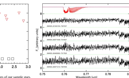
0.75 0.76 0.77 0.78 0.79 0 2 4 6 8 0.75 0.76 0.77 0.78 0.79 Wavelength [µm] 0 2 4 6 8 Fλ [arbitrary units] 2MASS J01003150−7307237 2MASS J00571648−7310527 2MASS J00493262−7317523 2MASS J00571214−7307045
Fig. 3.Illustrative spectra in the VIS wavelength range. The red
spec-trum is a telluric sky model, smoothed to R ∼ 10 000. From top to bottom, the stars are 2MASS J01003150-7307237, 2MASS J00571648-7310527, 2MASS J00493262-7317523 and 2MASS J00571214-7307045. Offsets of 0, 2, 4, 6 and 8 flux units have been applied to the C-star spectra and the telluric spectrum for display.
used apertures as large as possible (considering the need to es-timate the sky), sometimes at the expense of the signal-to-noise ratio of these wide-slit spectra. A number of the wide-slit ob-servations of carbon stars lacked significant signal (especially in ESO Period P84; cf. Table1), making it impossible to correct the higher resolution observations of these stars for slit losses.
3.3. Telluric correction and flux calibration
X-Shooter is a ground-based instrument. Therefore, we must correct our spectra for extinction by the Earth’s atmosphere. Standard flux calibration procedures account for continuous extinction, but not for molecular absorption lines (e.g., water vapour, molecular oxygen, carbon-dioxide, methane). Hereafter, we refer to these as telluric features. Telluric absorption features particularly affect the NIR arm and the reddest part of the VIS arm of X-Shooter.
3.3.1. VIS arm
The VIS spectra released in DR1 are already flux-calibrated and telluric corrected (Chen et al. 2014). For later periods, the flux calibration was performed within the X-Shooter pipeline. The telluric correction was applied afterwards. As for all cool stars in DR1, we selected telluric standard stars (with spectral types B and A) observed close in time and airmass to the carbon stars. We derived the telluric transmission spectra by removing the in-trinsic stellar spectrum, e.g., fitting and removing H lines and normalizing the continuum. The science spectra were then di-vided by the transmission spectra.
Figure3shows some of the spectra of the carbon stars over a small part of the visible wavelength range (0.07 µm wide). The red spectrum is a telluric model, arbitrarily chosen, shown for comparison.
3.3.2. NIR arm
The need for specific procedures to account and correct for tel-luric absorption is common to many NIR instruments. It is exa-cerbated in X-Shooter data by an unfortunate feature of the flat-field images. In the design of the pipeline, spectral features of the flat-field lamp remain present in the (globally) normalized flat-field images by which the data are divided and are propa-gated into the estimated instrument response curves. One such feature dominates over any other detector variations, a very strong and sharp bump in the K-band flatfielded spectra, with a much weaker secondary bump in the H-band (see, e.g., Fig. 9 of Moehler et al. 2014). At the altitude of the ESO Very Large Telescopes, water vapor absorption leaves broad gaps with no useable data in the NIR spectra, and only very few points any-where that are free of any telluric molecular absorption. The in-terpolation of estimated response curves through these gaps is a particularly poorly constrained exercise in the case of X-Shooter pipeline products because only relatively high-order polynomi-als can match the bumps due to the flat-field. Therefore, we de-signed a method to evaluate the response curve that explicitly ac-counts for telluric absorption.Moehler et al.(2014) andKausch et al.(2015) developed in parallel other implementations of this idea.
To model the telluric absorption, we chose to use the Cerro Paranal Sky Model, a set of theoretical telluric transmission spectra provided by J. Vinther and the Innsbruck team (Noll et al. 2012;Jones et al. 2013). These models are a more complete version of the spectra that can be found on the web application SkyCalc1,2.
The response curve was evaluated as follows. Because the flat-field bumps are variable in time, we required that the spec-trophotometric standard star used to derive a response curve for a given program star was reduced with the same flat-field ima-ges as that program star. We then fit the flat-fielded spectrum of the flux standard with the product of the theoretical spec-trum of this star, a telluric transmission model and the unknown response curve. Spectral regions with telluric features of inter-mediate depth were used to select the best-fitting telluric model within the available collection. The response curve was repre-sented with a spline polynomial, with higher concentrations of spline nodes where required by the flat-fielding bumps. We cor-rected the response curve for continuous atmospheric extinction using the Paranal extinction curve, as available in the X-Shooter pipeline directory, and taking into account the airmass of the flux standard.
For the subsequent correction of the narrow-slit spectra of carbon stars, the search of the “best” telluric model is also needed and more important than above (as we care not only about the shape but also about the lines). Therefore, instead of using one telluric model, we allowed for a larger variety of telluric transmissions by using linear combinations of principal components of the available telluric absorption models, selected within a range of airmasses similar to the airmass of the data. We performed the χ2minimization separately in four wavelength in-tervals3. The idea is to better target different molecules in the
luric spectra. Then, we divided the science spectrum by the tel-luric transmission and the response curve. We also corrected the
1 http://www.eso.org/observing/etc/bin/gen/form?INS.
MODE=swspectr+INS.NAME=SKYCALC
2 The files were computed with version 1.2 based on SM-01 Mod1
Rev.74, LBLRTM V12.2, and the line database was aer_v_3.2.
3 We use the following wavelength regions: 0.9–1.345 µm,
1.46–1.8 µm, 1.975–2.1 µm and 2.1–2.5 µm. 2.00 2.02 2.04 2.06 0 2 4 6 8 2.00 2.02 2.04 2.06 Wavelength [µm] 0 2 4 6 8 Fλ [arbitrary units] 2MASS J01003150−7307237 2MASS J00571648−7310527 2MASS J00493262−7317523 2MASS J00571214−7307045
Fig. 4.Illustrative spectra in the NIR wavelength range. The red
spec-trum is a telluric sky model, smoothed to R ∼ 8000. The stars are the same as in Fig.3.
science spectrum for continuous atmospheric extinction using the airmass at the time of observation.
Whenever possible, the final flux-calibrated spectra were ab-solutely flux-calibrated by using wide-slit (500) observations
(re-fer to column “Flux note” of Table1for exceptions).
Figure4shows the quality of our telluric correction process on some of our carbon stars. The red spectrum shows a telluric model for comparison.
3.4. Problem with the last order of NIR spectra
Some of our NIR observations, once flat-fielded, extracted, merged and flux-calibrated, display a step between the two red-dest orders (around 2.27 µm, between orders 12 and 11). This could be related to a known vignetting problem in order 11, i.e., the last order of the NIR arm that covers 2.28–2.4 µm, to the high background levels in certain exposures, or to other unidentified artifacts. Although we account for variation in the background emission along the slit in order 11 and we reduce pairs of one flux standard and one carbon star with the same flat-field, we cannot eliminate the step completely.
We correct for the discontinuity, when present, by forcing the average flux level between 2.28 and 2.29 µm in order 11 to match the extrapolation of a linear fit to the spectrum between 2.150 and 2.265 µm. This choice is guided by the aspect of theoretical spectra of C stars (Aringer et al. 2009) and by published obser-vations with other instruments (Lançon & Wood 2000;Rayner et al. 2009). Broad-band colors involving the Ks-band change by
(usually much) less than 2% with this correction. The estimated extra uncertainty on measures of the12CO bandhead within
or-der 11 remains below a few percent for weak bands, but can reach 10% for some of the stars with strong CO bands.
3.5. Final steps
We use theoretical models of carbon stars (R ∼ 200 000), com-puted specifically for this paper (based on the atmospheric mo-dels ofAringer et al. 2009), to shift the wavelength scale of our observed spectra to the vacuum rest-frame.
Finally, the three arms are merged to produce a complete spectrum from the near-UVB to the NIR4. The resolving power
in the UVB, VIS and NIR ranges of the merged spectra are, res-pectively, R ∼ 9100, ∼11 000 and ∼7770.
4. The diversity of carbon star spectra
Our sample of carbon stars presents quite a diversity in spec-tral shape and absorption-line characteristics. FiguresD.1toD.6
show our spectra from the UVB to the NIR wavelength range. The spectra were normalized to the flux at 1.7 µm and shifted for display purposes. The gray bands in the NIR mask regions where the telluric absorption is deepest and the signal cannot be recovered. It is important to note that the spectra were heavily smoothed to a common resolution (R ∼ 2000) in these figures.
We group our carbon stars by (J − K) values when describing them in the remainder of this Section. Figure5summarizes the spectral variety of the sample, showing representative examples of each group. The colors are used to better identify the different groups.
CO, CN and C2 produce the vast majority of features in
spectra of carbon stars in this wavelength range. Some bands have sharp bandheads, but a forest of lines from various transi-tions are spread across the whole spectrum. The C2Swan bands
(Swan 1857) are dominant between 0.4 and 0.6 µm. Longward of 0.6 µm, the most prominent bandheads are due to CN. Note that the NIR CN bands, in particular the 1.1 µm bandhead, are also seen in M giants and supergiants (Lançon et al. 2007;Davies et al. 2013). The C2band at 1.77 µm is one of the unambiguous
characteristics of C stars in the NIR. The CO bands in the H and K windows are also present with varying strengths in all the spectra.
First we describe spectral characteristics of each group seen from visual inspection. We perform a more quantitative analysis in subsequent sections.
4.1. Group 1 – The bluest stars: (J – K) < 1.2 [5 stars] Figure D.1shows the five warmest C stars in our sample. The top two spectra of Fig.5, displayed in blue, are representative of the two types of behaviors found in this group.
The top two stars of Fig.D.1, HD 202851 and HE 1428-1950, have spectra similar to those of early K type gi-ants (CN band at 0.431 µm and G band of CH of similar strength, Hβ line in absorption). But they clearly display the C2bands characte-ristic of C stars, in particular the Swan bands
around 0.47 µm and 0.515 µm.
The three bottom spectra of Fig. D.1have spectral energy distributions (SED) that peak at longer wavelengths, but have weaker molecular features in the optical range. The CN band at 0.431 µm and the G band of CH are undetectable in two of the three stars. On the other hand, the red system of CN is slightly stronger, and the NIR C2bandhead (1.77 µm) and the CO bands
are significantly stronger. Two of these three spectra display hy-drogen emission lines, a phase-dependent signature of pulsation. 4.2. Group 2 – Classical C stars: 1.2 < (J – K) < 1.6 [7 stars] Figure D.2 shows classical C stars: seven stars belong to this group. The third spectrum in Fig. 5 (2MASS J00571214-7307045), displayed in green, is representative of this group. All 4 The three arms overlap quite well: UVB: 0.3–0.59 µm; VIS:
0.53–1.02 µm; NIR: 0.99–2.48 µm.
these C stars have 1.2 < (J − K) < 1.6. They happen to be lo-cated in the SMC, but we note that many of the Galactic C stars ofLançon & Wood(2000) would fall in this category.
At optical wavelengths, the Swan bands are the first features to appear when C/O > 1. Compared to the first group of spectra, the spectra collected here have significantly stronger absorption bands of CN and C2in the NIR. C2absorption modifies the
spec-trum across the J band and creates a strong bandhead at 1.77 µm. A forest of lines of both CN and C2is responsible for the rugged
appearance of the spectrum, which should not be mistaken as an indication of noise. CO bands in the H window appear weak, as a combined consequence of the C/O ratio and of overlap with many other features.
The SED and the H band (CO, C2, forest of CN and C2
lines) of the top spectrum of Fig. D.2 (2MASS J01003150-7307237) seem to indicate that this star is slightly warmer, or has a lower C/O ratio, than the others. The opposite holds for the last spectrum in that figure.
4.3. Group 3 – Redder stars: 1.6 < (J – K) < 2.2 [13 stars] FiguresD.3andD.4show redder stars. Thirteen stars compose this group. Group 3 is less homogeneous than Group 2: while some spectra simply seem to extend the sequence of Group 2 to redder SEDs with stronger features, others deviate from this behavior. This leads us to define two subgroups. A representative of each subgroup is included in Fig.5(see the fourth and fifth spectra, displayed in orange).
The stars that simply extend the behavior of group 2 have strong C2 bands in the J- and H-bands and weak CO bands.
In two of these stars (T Cae and [W65] c2), the CO bands are re-latively stronger, suggesting a C/O ratio closer to 1 (cf. the S/C star BH Cru inLançon & Wood 2000). We warn however that the interpretation of ratios of CO to other band strengths in terms of abundance ratios is a non-trivial exercise, as the band-strength ratios may depend on phase (see the multiple spectra of R Lep byLançon & Wood 2000, or those of V Cyg fromJoyce 1998).
Two stars stand out: SHV 0500412-684054 and SHV 0502469-692418. They are characterized by an absorption band around 1.53 µm (see Sect.4.5), weaker C2absorption, some of
the strongest 2.3 µm CO absorption of this group, and a sig-nificantly smoother general appearance than other spectra. This latter property has, to our knowledge, never been emphasized before. In hindsight, it is also noticeable in previously published spectra that display the 1.53 µm feature (Lançon & Wood 2000;
Groenewegen et al. 2009;Rayner et al. 2009).
Inspection of the spectra with the 1.53 µm feature also sug-gests that their emission in the red part of the optical spectra is relatively strong, considering their red NIR spectra. The spectra however drop rapidly to a negligible flux in the blue.
4.4. Group 4 – The reddest stars: (J – K) > 2.2 [9 stars] The last two figures, Figs.D.5andD.6, show our reddest stars. The dichotomy seen in Group 3 is obviously present here as well. The two bottom spectra from Fig.5, displayed in red, are rep-resentative of that group, composed of nine stars. The general trend in this group is that the energy peak shifts from the optical to the near-infrared, which leads to a “plateau” in the K band of the reddest objects.
It is interesting to note that at higher (J − K), more stars display the 1.53 µm absorption feature. The fact that the feature
0.5
1.0
1.5
2.0
0
2
4
6
8
10
0.5
1.0
1.5
2.0
Wavelength [
µm]
0
2
4
6
8
10
F
λ[arbitrary units]
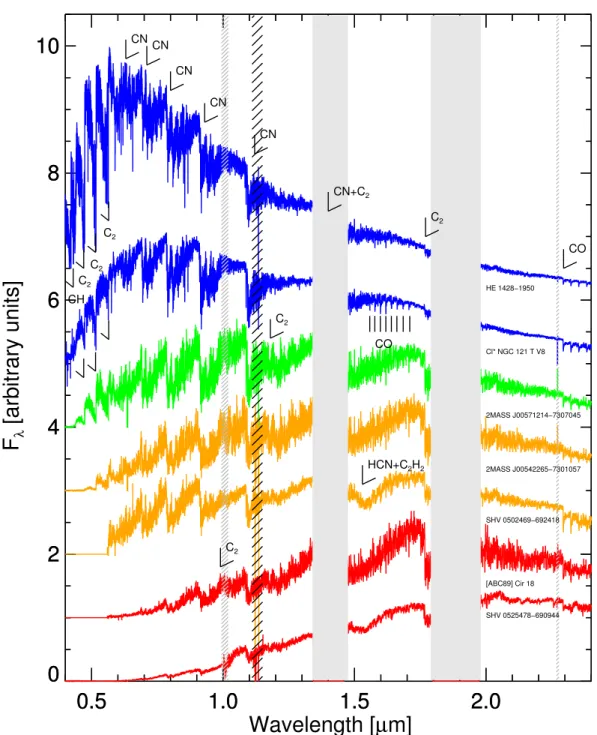
HE 1428−1950 Cl* NGC 121 T V8 2MASS J00571214−7307045 2MASS J00542265−7301057 SHV 0502469−692418 [ABC89] Cir 18 SHV 0525478−690944 CH C2 C2 C2 CN CN CN CN CN CN+C2 C2 CO C2 CO HCN+C2H2 C2Fig. 5.Representative spectra from our sample of carbon stars. The gray bands mask the regions where telluric absorption is strongest. The areas
hatched in black are those that could not be corrected for telluric absorption in a satisfactory way. The areas hatched in gray are the merging regions between the VIS and NIR spectra and between the last two orders of the NIR spectrum. In some spectra, data are missing at 0.635 µm. The spectra have been smoothed for display purposes to R ∼ 2000. The colors represent the different groups of carbon stars. Group 1 stars are shown in blue (from top to bottom: HE 1428-1950 and Cl* NGC 121 T V8), Group 2 in red (2MASS J00571214-7307045), Group 3 in orange (from top to bottom: 2MASS J00542265-7301057 and SHV 0502469-692418) and Group 4 in red (from top to bottom: [ABC89] Cir 18 and SHV 0525478-690944).
appears only in very red stars (but not in all very red stars) is con-sistent with previous observations (Joyce 1998; Groenewegen et al. 2009). The spectra that display 1.53 µm absorption share the properties already mentioned for their counterparts in Group 3. They clearly have a smoother appearance than the others. Unfortunately, the S/N ratio is poor for some of these ob-jects beyond 2.25 µm. Where it is good, inspection by eye indi-cates that the CO bands in these smoother spectra have strengths similar to those in spectra with a forest of CN and C2 lines.
In three cases, SHV 0520505-705019, SHV 0527072-701238,
SHV 0528537-695119, there seems to be an excess of flux in the red part of the optical spectrum, compared to other stars.
4.5. The 1.53µm feature
The 1.53 µm absorption feature was first noticed in cool carbon stars of the Milky Way (Goebel et al. 1981;Joyce 1998). These authors associated it with large-amplitude variability. The under-lying molecules are most likely a combination of HCN and C2H2
Table 2. Properties of our spectroscopic indices.
Index Bandpass feature λmin(µm) λmax(µm) Bandpass “continuum” λmin(µm) λmax(µm)
C2U C2U_band 0.5087 0.5167 C2U_cont 0.5187 0.5267
CN W110 1.0970 1.1030 W108 1.0770 1.0830
DIP153 DIP153_band 1.5000 1.6000 DIP153_cont 1.4800 1.5000
COH52 COH52_band 1.5974 1.6026 COH52_cont 1.5914 1.5966
COH63 COH63_band 1.6174 1.6226 COH63_cont 1.6114 1.6166
C2 C2_band 1.7680 1.7820 C2_cont 1.7520 1.7620
CO12 KH86CO1 2.2931 2.2983 KH86c1 2.2873 2.2925
CO13 KH86CO3 2.3436 2.3488 KH86CO2 2.3358 2.3410
be an overtone of the strong absorption band sometimes seen around 3 µm (e.g., in the spectrum of R Lep in the IRTF library). However, this correlation remains to be formally established, as
Joyce(1998) stated that this correlation is poor.
In our sample, all the spectra that display the 1.53 µm feature belong to large-amplitude variables. The fact that in our sample they all happen to be in the LMC should be seen as a selection effect, since stars with this feature have previously been found both in the Milky Way and in dwarf galaxies more metal-poor than the LMC (e.g., the Sculptor dwarf, Groenewegen et al. 2009).
5. Spectroscopic indices for carbon stars
We derive spectroscopic indices from our flux-calibrated spectra to compare our sample with previous studies. Unless otherwise stated, we use the following formula to measure the strength of any absorption band X:
I(X)= −2.5 log10[Fb(X)/Fc(X)], (1)
where Fb(X) and Fc(X) are the mean energy densities received
in the wavelength bin in the absorption band region and the (pseudo-)“continuum”5of index X.
We note here that these “one-sided” indices depend on the quality of the flux calibration over moderate wavelength spans, in contrast to the classic “two-sided” Lick/IDS-type indices such as those defined by, e.g.,Burstein et al.(1984), which are robust to small-scale flux-calibration issues. We evaluate error bars on indices by measuring them on spectra reduced with several es-timates of the instrumental response curve, and by taking the standard deviation of these measurements.
Table2summarizes the properties of the bandpasses used to define our spectroscopic indices, as illustrated in Figs.7–13. 5.1. Broad-band colors
For each of our spectra, we derived synthetic magnitudes using theBessell(1990) filters R and I and the 2MASS filters (Cohen et al. 2003) J, H and Ks. We use these magnitudes to define the
colors (R − H), (R − I), (I − H), (I − K), (J − H), (H − K) and (J − Ks).
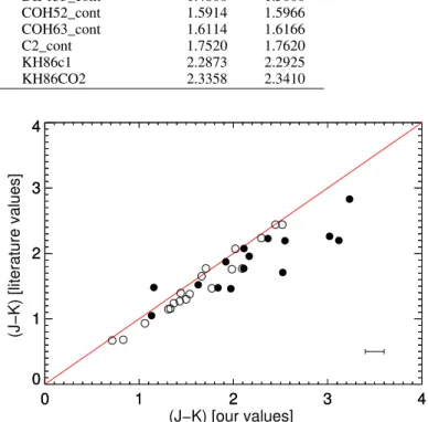
Figure6compares our (J − Ks) colors with those found in the
literature. When we exclude large-amplitude variables, we find a good agreement6. The dispersion increases with redder colors, 5 At the resolution of our C-star spectra, the true continuum is
inac-cessible anywhere. What we call pseudo-“continuum” in this section is simply a reference flux level measured outside the molecular band of in-terest for a particular spectrophotometric index, following earlier usage by, e.g.,Worthey et al.(1994).
6 The offset might be due to zero-point differences between our
syn-thetic photometry and the listed 2MASS magnitudes. Indeed, using the
0 1 2 3 4 0 1 2 3 4 0 1 2 3 4 (J−K) [our values] 0 1 2 3 4 (J−K) [literature values]
Fig. 6.Comparison of our (J − Ks) values with values found in the
li-terature (2MASS values,Cutri et al. 2003). The red line indicates the one-to-one relation. The black points represent the stars with large-amplitude (I large-amplitude ≥0.8). The bar plotted in the bottom-right corner shows the ±1σ root-mean-square deviation of our photometry with re-spect to the literature (large-amplitude variables excluded). This is an upper limit of the uncertainties in the flux calibration and any possible residual variability.
as already noted byWhitelock et al.(2009). The large scatter for the large-amplitude pulsators is not surprising, since we are com-paring our instantaneous color with 2MASS observations about ten years old, and many light curves display long term trends in addition to periodicity.
5.2.12CO indices
We first look at the CO bands located in the K band. To measure the12CO(2, 0) bandhead around 2.29 µm, we use the definition
given byKleinmann & Hall(1986): the absorption bandpass is centered on 2.295 µm (KH86c1) and the continuum bandpass is centered on 2.2899 µm (KH86CO1). We call this index CO12. Figure7shows these passbands on one of our spectra.
Other CO bands can also be found in the C-star spectra.
Origlia et al.(1993) studied the CO band in the H-band near 1.62 µm, corresponding to∆υ = 3 ro-vibrational bands. In our spectra, this 12CO(6, 3) line does not always appear. Figure8
reference fluxes for zero-magnitude stars inCohen et al.(1992) and a recent template Vega spectrum from the Hubble Space Telescope calibration documentation (ftp://ftp.stsci.edu/cdbs/current_
calspec/), our synthetic photometry gives (J − Ks)= 0 for Vega, while
2.280 2.285 2.290 2.295 2.300 2.305 2.310 0 1 2 2.280 2.285 2.290 2.295 2.300 2.305 2.310 Wavelength [µm] 0 1 2 Fλ [arbitrary units] CO12
Fig. 7. Zoom into the 12CO(2, 0) feature near 2.3 µm. The red line
indicates the region used to calculate the KH86CO1 bandpass, while the blue line corresponds to the KH86c1 bandpass measuring the continuum. This star is 2MASS J00571648-7310527.
shows two examples taken from our sample where the CO(6, 3) lines are seen (upper panel) or are hidden under a combination of CN and C2lines (lower panel).
We define a new index COH, based on two other indices measuring the12CO(5, 2) at 1.60 µm (COH52) and the12CO(6, 3)
line at 1.62 µm (COH63):
COH= (COH52+ COH63)/2. (2)
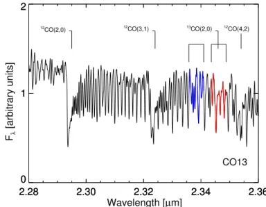
5.3.13CO index
The strongest 13CO features in the spectra are the ∆υ = 2
ro-vibrational bands located around 2.53 µm. To measure the
13CO(2, 0) bandhead, we use the definition of the bandpass
centered on 2.3462 µm given by Kleinmann & Hall (1986) (KH86CO3). We do not use the same definition for the conti-nuum as their bandpass is centered on 2.2899 µm and thus too far away from the absorption bandpass and more likely to be sensitive to slope effects. Therefore, we define a new bandpass for the continuum and create the index CO13. Figure9 shows the definition of the bands used to define this index on one of our spectra.
5.4. CN index
CN is also seen in carbon-rich spectra. The red system of CN appears beyond 0.5 µm and the bands grow towards longer wavelengths. To estimate the CN in the NIR part of the spec-trum, we use rectangular filters adapted from the 8-color system of Wing(1971). We use an index CN, based on Wing’s W110 and W108 passbands, that measures the CN feature at 1.1 µm. Figure10shows these passbands.
5.5. Measure of the 1.53µm feature
Some of our stars exhibit the 1.53 µm feature. We interpret this feature to be caused by HCN+C2H2. We define an index DIP153
to measure its depth. Figure11shows two examples taken from
0 1 2 0 1 2 Fλ [arbitrary units] COH52 COH63 1.59 1.60 1.61 1.62 Wavelength [µm] 0 1 Fλ
[arbitrary units] COH
Fig. 8.Zoom into the12CO(6, 3) line near 1.62 µm. The red lines
indi-cate the features regions, while the blue measure the continuum. The upper panel shows the spectrum of a carbon star, Cl* NGC 121 T V8, in which the12CO(5, 2) and12CO(6, 3) bands are visible. The lower
panel corresponds to another carbon star, 2MASS J00571214-7307045, in which the CN and C2 lines are more prominent and overlap with
the CO lines. The spectra have been normalized at 1.62 µm for display purposes. 2.28 2.30 2.32 2.34 2.36 0 1 2 2.28 2.30 2.32 2.34 2.36 Wavelength [µm] 0 1 2 Fλ [arbitrary units]
12CO(2,0) 12CO(3,1) 13CO(2,0) 12CO(4,2)
CO13
Fig. 9.Zoom into the13CO(2, 0) line near 2.35 µm. The red line
in-dicates the region used to calculate the KH86CO3 bandpass, while the blue line corresponds to the KH86CO2 bandpass measuring the continuum. This star is SHV 0500412-684054.
our sample where this feature is seen (upper panel) and absent (lower panel).
5.6. C2indices
C2 bands appear at many wavelengths in the spectra of
car-bon stars. The bands between 0.4 and 0.7 µm correspond to the Swan system (Swan 1857). The C2bands at 0.77, 0.88, 1.02
and 1.20 µm are part of the Phillips system (Phillips 1948). The Ballik-Ramsay fundamental band is the C2 band
1.07 1.08 1.09 1.10 1.11 0 1 2 1.07 1.08 1.09 1.10 1.11 Wavelength [µm] 0 1 2 Fλ [arbitrary units] CN
Fig. 10.Zoom into the CN line near 1.1 µm. The red line indicates the
region used to calculate the W110 bandpass, while the blue line cor-responds to the W108 bandpass measuring the continuum. This star is SHV 0502469-692418. 0.2 0.8 1.4 0.2 0.8 1.4 Fλ [arbitrary units] HCN 1.50 1.55 1.60 1.65 1.70 1.75 Wavelength [µm] 0.2 0.8 Fλ [arbitrary units]
Fig. 11.Zoom into the HCN+C2H2 lines around 1.53 µm. The upper
panel shows an example of a carbon star, SHV 0502469-692418, in which the HCN+C2H2 feature is visible. The lower panel corresponds
to another carbon star, T Cae, in which the feature is missing. The red line indicates the region used to calculate the absorption bandpass, while the blue line corresponds to the continuum bandpass.
same definition asAlvarez et al.(2000). The bandpasses used to define the C2 index are shown in Fig.12.
The upper-right panel of Fig.13shows the C2Swan system
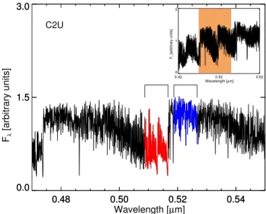
for one of our spectra. Due to low signal-to-noise for the XSL carbon stars at short wavelengths, the bands near 0.47 µm or bluer are barely seen. The band near 0.56 µm is problematic be-cause of instrumental issues in that range (Chen et al. 2014), and the bands above 0.6 µm are too heavily contaminated by CN. This leaves the band near 0.5165 µm as our best choice to define an index, even though this index cannot be defined for all stars of our sample due to an absence of signal in the UVB/VIS parts of some of our spectra. We call this index C2U.
1.75 1.76 1.77 1.78 1.79 0 1 2 1.75 1.76 1.77 1.78 1.79 Wavelength [µm] 0 1 2 Fλ [arbitrary units] C2
Fig. 12.Zoom into the C2 line around 1.77 µm. The red line indicates
the region used to calculate the C2_band bandpass, while the blue line corresponds to the bandpass measuring the continuum. This star is 2MASS J00563906-7304529. 0.48 0.50 0.52 0.54 0.0 1.5 3.0 0.48 0.50 0.52 0.54 Wavelength [µm] 0.0 1.5 3.0 Fλ [arbitrary units] C2U 0.42 0.52 0.62 Wavelength [µm] 0 1 2 Fλ [arbitrary units]
Fig. 13.The C2 Swan system (top panel) and a zoom into the C2 line
around 0.5165 µm. The red line indicates the region used to calculate the C2U_bandbandpass, while the blue line corresponds to the C2U_cont bandpass measuring the continuum. This star is HE 1428-1950.
5.7. Measure of the high-frequency structure
We also estimate the high-frequency structure in the H and Kbands, inspired by the smooth appearance of the NIR spectra of C stars with the 1.53 µm feature. For both windows, we first fit a straight line on the wavelength range under study: 1.66–1.7 µm for the H band and 2.18 – 2.23 µm for the K band. We then di-vide our spectrum by this fit, thus normalizing the continuum. Next, for any window X, we derive the rms from the following formula: rms(X)= s PN i(Xi− 1)2 N · (3)
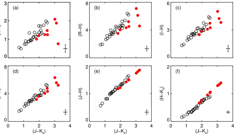
0 1 2 3 0 1 2 3 (R−I) (a) 0 4 8 (R−H) (b) 0 3 6 (I−H) (c) 0 1 2 3 4 (J−Ks) 0 4 8 (I−K) (d) 0 1 2 3 4 (J−Ks) 0 1 2 (J−H) (e) 0 1 2 3 4 (J−Ks) 0 1 2 (H−K s ) (f)
Fig. 14.Some color–color plots derived from our sample of carbon stars. The red circles stand for carbon stars showing the 1.53 µm feature. For
the R filter, we adopt some conservative values. The bars plotted in the bottom-right corners are determined as in Fig.6.
6. Results
6.1. Color–color plots
Figure14shows the locus of the observed carbon stars in color– color diagrams, based on the measurements made in Sect.5.1. On the whole, different colors are well correlated with each other. The dispersion along the trend is smaller at bluer colors.
The red circles stand for carbon stars showing the 1.53 µm feature in their spectra. A trend characterizes these stars in the color–color diagrams: at a given (J − Ks), they are bluer when
looking at color indices that involve R or I. We note that only panels b, c, e and f show colors that include the H band, which hosts the 1.53 µm feature itself. The separation between stars showing the 1.53 µm feature and classical C stars, however, is present in all the panels.
This separation into two groups reflects the results of visual inspection in Sect.4. Stars with the 1.53 µm feature tend to have excess flux at the red end of the optical spectrum, for a given energy distribution at farther NIR wavelengths.
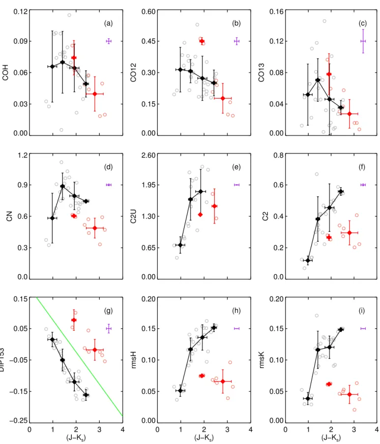
6.2. Molecular indices versus color
Figure 15 shows all the indices previously defined as a func-tion of (J − Ks). For each group of (J − Ks) (cf. Sect. 4), we
calculate the average values of each index and display them as filled symbols. The error bars indicate the 1σ standard devia-tions. We separate the red C stars from Groups 3 and 4 into two sub-groups: those with the 1.53 µm feature and those without.
Panels a to c in Fig.15display the CO indices as a function of (J − Ks). The data points are highly dispersed, with a marginal
trend of decreasing12CO indices when (J − K
s) increases.
In the H-band, the prominence of the CO bands in carbon star spectra depends on the strength of the CN and C2 bands.
These, in turn, depend on effective temperature, but also on the C/O ratio (Fig. 3 of Loidl et al. 2001). While strong in S and S/C stars (Rayner et al. 2009;Lançon & Wood 2000), the H-band CO features become indistinguishable in the forest of CN and C2lines at large C/O. In addition, the CO band strengths
anticorrelate with surface gravity (Origlia et al. 1993). In view of the many parameters that may control the amplitude of the related dispersion of COH values (others could include metal-licity, microturbulence, convection), our sample is too small to consider the trend with (J − Ks) significant.
At 2.29 µm, contamination by features other than CO is reduced but not negligible. Again, we believe the trend with (J − Ks) is only marginal. Anticipating later discussions, it is
interesting to note that two of the stars with the 1.53 µm feature are among those with the highest values of CO12.
Our measurements of13CO approach 0 above (J − Ks) ' 2,
and its detection is only significant in a few relatively blue stars. To some extent, this results from contamination of the measure-ment bandpasses by a forest of lines from other molecules and to measurement uncertainties beyond 2.25 µm. But weak13C
abun-dances are also a natural and well known result of the third dredge-up, which brings freshly synthesized12C to the surface
(Lloyd Evans 1980;Bessell et al. 1983).
Panel d shows the result for the CN index. The behavior is not monotonic. First, the strength of the CN index increases, up to (J − Ks) ' 1.6. Then, for redder stars, the CN bandhead slowly
fades. For stars with (J − Ks) ≥ 2, the sources with the 1.53 µm
absorption feature are clearly separated from the classical carbon stars.
0.00 0.03 0.06 0.09 0.12 COH (a) 0.00 0.15 0.30 0.45 0.60 CO12 (b) 0.00 0.04 0.08 0.12 0.16 CO13 (c) 0.0 0.3 0.6 0.9 1.2 CN (d) 0.00 0.65 1.30 1.95 2.60 C2U (e) 0.0 0.2 0.4 0.6 0.8 C2 (f) 0 1 2 3 4 (J−Ks) −0.25 −0.15 −0.05 0.05 0.15 DIP153 (g) 0 1 2 3 4 (J−Ks) 0.00 0.05 0.10 0.15 0.20 rmsH (h) 0 1 2 3 4 (J−Ks) 0.00 0.05 0.10 0.15 0.20 rmsK (i)
Fig. 15.Some indices derived from our sample of carbon stars as a function of (J − Ks). The red circles stand for the carbon stars with the 1.53 µm
feature. The filled diamonds represent the averaged values of our indices as a function of the bin number based on (J − Ks), and the bars measure
the dispersion within bins. Typical uncertainties on individual measurements are shown in purple.
Panels e and f display the C2indices. The C2U index is not
defined for the reddest objects in the sample because of a lack of signal at the relevant short wavelengths. The strength of both C2
indices increase with increasing (J − Ks) and drop down for the
reddest (J − Ks) values. The stars with the 1.53 µm absorption
feature behave differently (weaker C2bands, for a given (J−Ks)).
Panel g shows the index measuring the strength of the 1.53 µm feature as a function of (J − Ks). There is a clear
separation between stars with the 1.53 µm feature (red points) and the others. We add a green line showing this separation for later comparisons.
The last two panels h and i display the results for the measure of the high-frequency structure in the H and K bands. The con-tribution of observational errors to the measured rms indices is in general smaller than 0.02. As expected, the values of the rms in-crease with increasing (J −Ks), but stars with the 1.53 µm feature
follow the opposite trend. The quantitative assessment supports the conclusion drawn from visual inspection (see Figs.D.1and following).
7. Comparison with the literature
Figures16and17compare our sample of carbon stars with exis-ting libraries.
7.1. Spectra fromLançon & Wood(2000)
A widely-used library containing carbon stars is that constructed by Lançon & Wood (2000, hereafter LW2000). They built a library of spectra of luminous cool stars from 0.5 to 2.5 µm, which includes 7 carbon stars. In addition, their data include multiple observations of individual variable stars. One of their stars, R Lep, is a large-amplitude variable star, which exhibits the 1.53 µm feature. The different observations of this star are represented as filled magenta stars in Figs.16and 17.
7.2. Spectra fromGroenewegen et al.(2009)
We also compare our spectra with spectra observed by
Groenewegen et al. (2009). They observed carbon rich AGB stars in the Fornax and Sculptor dwarf galaxies. The obser-vations covered the entire J- and H-band atmospheric win-dows. This sample is particularly interesting as their color-selected sample happened to contain several carbon stars with the 1.53 µm feature. Table 3 summarizes properties of their carbon stars: 2MASS J, H and Ks magnitudes and also the
strength of the 1.53 µm feature, as available from Table 1 of
Groenewegen et al. (2009). Based on their classification, stars for which this feature is “medium,” “strong” or “extreme” are represented as filled blue triangles in Figs.16and17.
7.3. Spectra from IRTF (Rayner et al. 2009)
Finally, we compare our carbon stars with those from the IRTF Spectral Library (Rayner et al. 2009, hereafter IRTF). Their col-lection counts 8 C-star spectra from 0.8 to 5.0 µm, including R Lep. In Figs. 16 and17, this star is represented as a filled green square.
7.4. Results
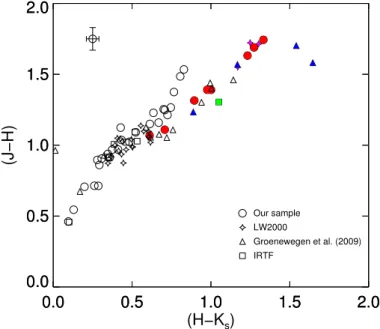
Figure 16 shows the color–color diagram of (J − H) versus (H − Ks) for our sample of carbon stars (circles), to which we
add the C stars from LW2000 (stars),Groenewegen et al.(2009) (triangles) and IRTF (squares). The colored symbols represent the carbon stars with the 1.53 µm feature. All the colors, except those fromGroenewegen et al.(2009), were rescaled to 2MASS values for consistency in our comparison7. It is interesting to 7 The colors were rescaled by the following factors:
(J − H)new= (J − H)ori− 0.10;
0.0
0.5
1.0
1.5
2.0
0.0
0.5
1.0
1.5
2.0
0.0
0.5
1.0
1.5
2.0
(H−K
s)
0.0
0.5
1.0
1.5
2.0
(J−H)
Our sample LW2000 Groenewegen et al. (2009) IRTFFig. 16.The spread of our sample of carbon stars (circles) in the (J−H)–
(H − Ks) color–color plane. The star symbols represent LW2000, the
triangles representGroenewegen et al.(2009) and the squares represent IRTF. Colored symbols stand for those carbon stars with the 1.53 µm feature.
note that the 1.53 µm feature makes the stars fainter in H, so stars with this feature are bluer in (J − H) and redder in (H − Ks).
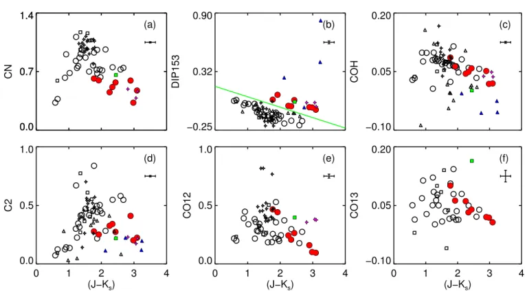
We compute for the three samples of carbon stars under study the spectroscopic indices just like for the XSL spectra. Figure17 shows six of our indices as a function of (J − Ks).
Not all the indices are defined for the stars fromGroenewegen et al.(2009), as their spectra are confined to the J and H bands. Panel a shows the result for the CN index. The trend is as in Fig.15: an increase of the CN band up to (J − Ks) ' 1.6 and then
a slow decrease at redder colors.
Panel b shows the result for the DIP153 index. The green line is the same line as in panel g of Fig.15. Our criterion to identify stars with the 1.53 µm feature appears to be reasonable when applied to a larger sample.
In the same panel, one star identified with a star symbol and not explicitly identified as containing HCN+C2H2 appears
close to the group of stars with the 1.53 µm feature. This star is BH Cru, a Galactic star, with spectral type CS. Its IRAS-LRS spectrum shows that it is not surrounded by a lot of dust (“a hint of circumstellar emission” as mentioned byLambert et al. 1990). This star displays exceptionally strong CO bands in the H-band and these contaminate the DIP153 index (see Fig. B28 ofLançon & Wood 2000).
Panel c plots the COH index. We still observe a decrease of the strength of the COH as (J − Ks) increases.
Panel d shows the C2 index. The most of the “normal” stars seem to lie on a sequence, while the stars with this 1.53 µm fea-ture are all gathered in the lower right-hand quarter of the plot.
Panels e and f display the CO12 and CO13 indices. The gen-eral trend is a decrease of those two indices as (J − Ks) increases.
(H − Ks)new= (H − Ks)ori− 0.05;
0.0 0.7 1.4 0.0 0.7 1.4 CN (a) −0.25 0.32 0.90 DIP153 (b) −0.10 0.05 0.20 COH (c) 0 1 2 3 4 (J−Ks) 0.0 0.5 1.0 C2 (d) 0 1 2 3 4 (J−Ks) 0.0 0.5 1.0 CO12 (e) 0 1 2 3 4 (J−Ks) −0.10 0.05 0.20 CO13 (f)
Fig. 17.Six of our indices as functions of (J − Ks). Symbols and colors are as in Fig.16.
8. Discussion
8.1. The bluest stars
In Sect. 4.1, we described the 5 bluest carbon star spectra of our sample (Fig. D.1). For the top two stars, HD 202851 and HE 1428-195, effective temperatures available in the literature are above 4500 K (Bergeat et al. 2002;Placco et al. 2011). Hence these are unlikely to be classical C stars on the AGB. Formation scenarios with mass transfer from binary companion are more plausible.
The other three stars of the group (Cl* NGC 121 T V 8, SHV 0518161-683543 and SHV 0517337-725738) cannot be modeled as reddened versions of the previous two with standard reddening laws. The energy distributions do not match, and in addition circumstellar dust is not expected to play a major role around stars this warm. These three stars are intrinsically red-der than the first two and most likely do belong to the AGB. Only a detailed comparison with models will provide estimates of their parameters (Gonneau et al., in prep.). A redder SED can indicate a cooler effective temperature. Differences in the depth of the molecular bands can be the result of different metallicities and/or C/N/O abundance ratios. Luminosity may also play a role as the strengths of the CO and CN bands tend to increase when surface gravities drop.
One might be tempted to consider environmental effects, as the bottom three spectra of Fig.D.1belong to stars in the Large and Small Magellanic Clouds while the top two are in the Milky Way. But one of the two top spectra belongs to a Galactic Halo star (HE 1428-1950, Goswami et al. 2010), and is likely also of subsolar metallicity (Kennedy et al. 2011). It is unknown to which MW population the second top star belongs.
Finally, we note that two of these five spectra clearly display Hβ in absorption, and two others Hβ in emission. Hydrogen de-ficiency is unlikely to be an important characteristic of any of the stars in this group. Hydrogen emission is a known transient
Table 3. Carbon stars fromGroenewegen et al.(2009).
Star J H Ks Strength of
identifier 2MASS 2MASS 2MASS the 1.53 µm feature Fornax11 15.034 13.981 13.261 absent Fornax13 14.485 13.377 12.618 weak Fornax15 15.790 14.556 13.668 strong Fornax17 14.745 13.689 13.072 weak Fornax20 15.131 13.732 12.728 weak Fornax21 15.424 14.122 13.182 weak Fornax24 15.601 14.162 13.167 weak Fornax25 14.722 13.262 12.120 weak Fornax27 14.441 13.365 12.694 absent Fornax31 16.052 14.483 13.315 medium Fornax32 14.789 13.664 13.076 absent Fornax34 16.106 14.525 12.879 extreme Fornax-S99 14.677 13.749 13.427 absent Fornax-S116 15.004 14.041 14.028 absent Scl6 14.846 13.144 11.603 strong Scl-Az1-C 14.713 14.040 13.871 weak
property of pulsating variables, usually interpreted as the results of shocks in the extended atmospheres.
8.2. The bimodal behavior of red carbon stars
The previous sections have pointed out a bimodal behavior among carbon stars with redder near-infrared colors. The pre-sence or abpre-sence of the 1.53 µm absorption feature separates the two types of behaviors (at least in the XSL sample).
Figure 18 shows two of our high-resolution C-star spec-tra with similar (J − Ks) (of '1.85). The 1.53 µm feature is
present in the top spectrum but not in the bottom one. In ad-dition to the HCN+C2H2 feature, the top spectrum shows a
0.5 1.0 1.5 2.0 0.0 1.6 3.2 4.8 0.5 1.0 1.5 2.0 Wavelength [µm] 0.0 1.6 3.2 4.8 Fλ [arbitrary units] HCN+C2H2 SHV 0500412−684054 2MASS J00542265−7301057
Fig. 18.Two high-resolution, high signal-to-noise ratio C-star spectra
for which (J − Ks) ' 1.85. Only the top spectrum exhibits the 1.53 µm
feature. It also appears smoother in the near-infrared than the bottom one, and it has a peculiar energy distribution. The gray bands mask the regions where telluric absorption is strongest. The areas hatched in black are those that could not be corrected for telluric absorption in a satisfactory way. The areas hatched in gray are the merging regions between the VIS and NIR spectra, and between the last two orders of the NIR part.
two components, one peaking at red optical wavelengths, the other at long wavelengths.
What might explain this bimodal behavior? Groenewegen et al. (2009) have already discussed the anti-correlation be-tween the strength of the 1.53 µm feature and the C2
band-head at 1.77 µm. As the 1.53 µm feature is likely carried in part by C2H2, they have suggested the formation of this
com-plex molecule occurs at the expense of C2 when the C/O ratio
and the physical conditions are appropriate. While we have no argument against this suggestion, other parameters are needed to explain the effects we see in the overall SED and the anti-correlation with the apparent strength of the forest of lines in the H- and K-bands.
Two of the main fundamental parameters of carbon star mo-dels are the effective temperature and the C/O ratio. Aringer et al.(2009) showed that dust-free hydrostatic models with any reasonable values for these parameters fail to reproduce stars redder than (J − Ks) ' 1.6. Circumstellar dust is invoked to
ex-plain redder objects. At optical and NIR wavelengths, this dust is usually thought of as a cause of extinction (Lançon & Mouhcine 2002; Lloyd Evans 2010). But extinction by itself cannot ex-plain the phenomenon we observe. All classical extinction laws are monotonic functions of wavelength through the optical and NIR range. They cannot explain that, at a given (J − Ks), stars
with the 1.53 µm feature have an apparent peak in their Fλenergy
distribution in the red part of the optical spectrum.
One explanation for both the SED and the apparent smoothness of the peculiar spectra in the NIR range (e.g., SHV 0500412-684054) is an additional continuous emission component at NIR wavelengths. While the emission component of the veiling by circumstellar dust is usually detected only at longer, mid-infrared wavelengths for mass-losing AGB stars, the particular instantaneous structure around some stars may lead to a significant contribution in the near-infrared. An additive continuum reduces the equivalent width of absorption features
in the composite spectrum, resulting in a smoother appearance. Indeed, such a dilution is seen at NIR wavelengths in some of the spectra of dusty pulsating C-star models ofNowotny et al.
(2011,2013), although this aspect was not pointed out by the authors. Furthermore the existence of objects dominated by dust emission at NIR wavelengths such as V CrA (Fig.A.2) hints at intermediate situations.
If we accept the idea of continuous thermal dust emission in the NIR, we should expect all near-infrared photospheric mole-cular bands to be similarly weakened. That would explain the weaker C2and CN bands. The stronger HCN+C2H2absorption
suggests that these molecules are intermixed with the dust high above the region responsible for the other absorption bands. A similar argument was made bySloan et al.(2006) andZijlstra et al.(2006). As the CO bands around 2.3 µm do not seem to be weakened as much as the C2or CN lines, CO is also inferred
to exist at circumstellar radii at least as large as the emitting dust. This is compatible with dynamical models of carbon star atmospheres, which indicate that the robust CO molecule exists throughout the circumstellar environment, and the CO(2, 0) lines originate around the radii of dust production, i.e., where most of the NIR dust emission is likely to be produced (Nowotny et al. 2005).
Indeed, for dust to emit at NIR wavelengths, it must be rela-tively hot and located near the star. This is most likely to happen when the dust first forms, and to last only until that dust shell is carried farther out into cooler regions. Why the presence of dust emission seems to correlate so well with the presence of the 1.53 µm feature would remain to be explained by a renewed look at models of the chemical structures of pulsating atmospheres.
It is also interesting to note that all the stars in our sam-ple with the 1.53 µm absorption band are Miras8 but not all
the Miras have this feature (see Table B.1 for more details). Large-amplitude pulsation might thus be a requirement for dust to be forming via a particular chanel, associated with the NIR signatures of HCN and C2H2 and with relatively hot dust
temperatures.
Sloan et al.(2015) andReiter et al.(2015) recently empha-sized another example of the connection between the spectral properties and the pulsation mode of carbon stars: the long pe-riod variables separate into two sequences when plotting the mid-infrared [5.8]–[8] color versus (J − Ks). Nearly all
semi-regular variables (SRV) follow a blue sequence with (J−Ks) <∼ 2,
while Miras dominate a redder sequence. In the range of overlap, around (J − Ks) ' 1.8, SRVs have larger [5.8]–[8] color indices
than Mira variables, which the authors relate to the presence of a strong C3absorption band around 5 µm in SRVs. The
compe-tition between C3, C2, HCN, and C2H2, as well as the relations
between their abundances, their band strengths, the stellar pulsa-tion amplitude, and the instantaneous atmospheric structure, are interesting open questions for future statistical studies.
Finally, we note that this discussion does not account for the effects of circumstellar kinematics on line profiles. Velocity differences larger than 15 km s−1 within the molecular line
formation regions of long-period variables lead to complex broadened line profiles (Nowotny et al. 2005), which will affect spectra observed at the resolution of X-Shooter. This has been 8 This is also the case for the stars with 1.53 µm absorption observed
byGoebel et al.(1981),Joyce(1998),Lançon & Wood(2000). Among
the 9 C stars inGroenewegen et al. (2009) with this absorption and with some amplitude information (mostly fromWhitelock et al. 2009) at least four are Miras. Two are labeled “semi-regular with long term trends”, three others have quoted J-band amplitudes of 0.6, 1.0 and 1.0 in that article.