HAL Id: hal-00305061
https://hal.archives-ouvertes.fr/hal-00305061
Submitted on 27 Feb 2007
HAL is a multi-disciplinary open access
archive for the deposit and dissemination of
sci-entific research documents, whether they are
pub-lished or not. The documents may come from
teaching and research institutions in France or
abroad, or from public or private research centers.
L’archive ouverte pluridisciplinaire HAL, est
destinée au dépôt et à la diffusion de documents
scientifiques de niveau recherche, publiés ou non,
émanant des établissements d’enseignement et de
recherche français ou étrangers, des laboratoires
publics ou privés.
streamflow volume forecasts
T. Hashino, A. A. Bradley, S. S. Schwartz
To cite this version:
T. Hashino, A. A. Bradley, S. S. Schwartz. Evaluation of bias-correction methods for ensemble
stream-flow volume forecasts. Hydrology and Earth System Sciences Discussions, European Geosciences
Union, 2007, 11 (2), pp.939-950. �hal-00305061�
www.hydrol-earth-syst-sci.net/11/939/2007/ © Author(s) 2007. This work is licensed under a Creative Commons License.
Earth System
Sciences
Evaluation of bias-correction methods for ensemble streamflow
volume forecasts
T. Hashino1, A. A. Bradley2, and S. S. Schwartz3
1University of Wisconsin, Department of Atmospheric and Ocean Sciences, Madison, WI, USA 2The University of Iowa, IIHR – Hydroscience & Engineering, Iowa City, IA, USA
3Center for Urban Environmental Research and Education, UMBC, Baltimore, MD, USA Received: 19 January 2006 – Published in Hydrol. Earth Syst. Sci. Discuss.: 27 April 2006 Revised: 18 August 2006 – Accepted: 23 February 2007 – Published: 27 February 2007
Abstract. Ensemble prediction systems are used opera-tionally to make probabilistic streamflow forecasts for sea-sonal time scales. However, hydrological models used for ensemble streamflow prediction often have simulation biases that degrade forecast quality and limit the operational use-fulness of the forecasts. This study evaluates three bias-correction methods for ensemble streamflow volume fore-casts. All three adjust the ensemble traces using a trans-formation derived with simulated and observed flows from a historical simulation. The quality of probabilistic fore-casts issued when using the three bias-correction methods is evaluated using a distributions-oriented verification ap-proach. Comparisons are made of retrospective forecasts of monthly flow volumes for a north-central United States basin (Des Moines River, Iowa), issued sequentially for each month over a 48-year record. The results show that all three bias-correction methods significantly improve forecast qual-ity by eliminating unconditional biases and enhancing the potential skill. Still, subtle differences in the attributes of the bias-corrected forecasts have important implications for their use in operational decision-making. Diagnostic veri-fication distinguishes these attributes in a context meaning-ful for decision-making, providing criteria to choose among bias-correction methods with comparable skill.
1 Introduction
In recent years, ensemble prediction systems (EPSs) have gained popularity in hydrological and meteorological fore-casting. EPSs produce forecasts based on multiple realiza-tions from a forecast model; the set of realizarealiza-tions is referred to as an ensemble. For example, the U.S. National Weather Service (NWS) is implementing an EPS for seasonal stream-Correspondence to: A. A. Bradley
flow forecasting as part of its Advanced Hydrologic Pre-diction Services (AHPS) (Connelly et al., 1999; McEnery et al., 2005). Historical weather data are used to simulate an ensemble of streamflow time series (traces) conditioned on the current hydroclimatic state. Frequency analysis is then applied to the ensemble traces, producing probability distribution forecasts for streamflow variables. Other recent examples using ensemble prediction techniques in stream-flow forecasting and water resources decision-making in-clude Georgakakos et al. (1998), Hamlet and Lettenmaier (1999), Carpenter and Georgakakos (2001), Faber and Ste-dinger (2001), Kim et al. (2001), Yao and Georgakakos (2001), Hamlet et al. (2002), Wood et al. (2002), Franz et al. (2003), Souza Filho and Lall (2003), Clark and Hay (2004), Grantz et al. (2005), and Roulin and Vannitsem (2005), among others.
One factor that can seriously affect the quality of EPS forecasts is model bias. For example, a hydrological model may systematically overestimate flows during baseflow con-ditions, or systematically underestimate peak flows for sum-mer thunderstorms. Model biases can result from the in-put data, the estimated model parameters, or simplifying as-sumptions used in the model. Regardless, biases from the forecast model will propagate to each trace in the ensemble, degrading the overall quality of the resulting forecasts. Bi-ases in streamflow ensemble traces also limit their use in wa-ter resources decision-making; biases need to be removed be-fore the traces are used as input to a decision support model. There are several ways of dealing with model biases in streamflow forecasting. One is to shift (or transform) the probability distribution forecast derived from the ensemble traces. This approach accounts for biases in forecast vari-ables, but the ensemble traces themselves are uncorrected. Another approach is to use a bias-correction transformation to adjust all model-simulated ensemble traces. The bias-corrected traces are then used to make the probability distri-bution forecast. This second approach is generally preferred
0 1000 2000 3000 4000 5000 6000 Dec Nov Oct Sep Aug Jul Jun May Apr Mar Feb Jan Volume (cms-days) Month
Des Moines River at Stratford, Iowa
Mean Standard Deviation
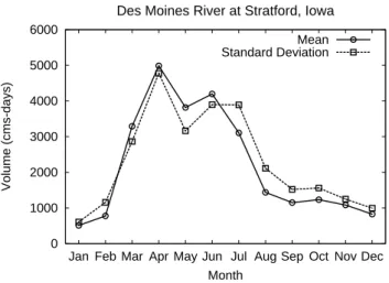
Fig. 1. Historical variations in monthly streamflow for the Des
Moines River at Stratford, Iowa (USGS 05481300). The plot shows the mean and standard deviation of monthly flow volume (cms-days) based on the stream-gage record from 1949 through 1996.
for streamflow forecasting, since bias-corrected ensemble traces can be utilized in water resources applications.
In this study, we evaluate three bias-correction methods for ensemble traces. Our approach is to assess the quality of the probabilistic forecasts produced with the bias-corrected ensemble. The evaluation is based on ensemble forecasts of monthly streamflow volume for a north-central United States basin (Des Moines River, Iowa). The distributions-oriented verification approach, originally proposed by Murphy and Winkler (1987), is utilized as a diagnostic framework for as-sessing forecast quality.
2 Experimental design
The evaluation of bias-correction methods for monthly streamflow forecasting is carried out using an experimental system for the Des Moines River basin in Iowa (Hashino et al., 2002). A hydrologic forecast model is used to make retrospective ensemble forecasts of monthly flow volume over the historical record (from 1949 through 1996). Three bias-correction methods are then applied to ensemble vol-umes, and ensemble forecasts are recomputed with the bias-corrected traces. Finally, the forecast quality of the retro-spective forecasts, with and without bias correction, are eval-uated.
2.1 Study area
The forecast location for this study is the Des Moines River at Stratford, Iowa (U.S. Geological Survey stream-gage 05481300). This location drains a 14 121 km2area, and is directly upstream of Saylorville Reservoir. Figure 1 shows the historical variations of the observed monthly flow volume at this site. Average flows are relatively high from March to
Table 1. Mean error (ME), root mean square error (RMSE), and
correlation coefficient (ρ) for a 48-year continuous simulation of monthly flow volumes for the Des Moines River at Stratford.
Month ME(%) RMSE(%) ρ
Jan 20.0 83.9 0.831 Feb 43.1 82.6 0.921 Mar −7.1 43.4 0.870 Apr −12.9 28.9 0.967 May −13.5 31.4 0.946 Jun −19.9 36.0 0.952 Jul −6.0 32.5 0.970 Aug 30.9 52.4 0.957 Sep 43.1 61.8 0.950 Oct 16.9 59.3 0.893 Nov 2.2 41.4 0.935 Dec −7.2 63.7 0.866
July. Snowmelt and low evapotranspiration produce signif-icant runoff in the spring, and wet soils and heavier warm season rains continue to produce significant runoff into the early summer. In contrast, monthly flows are relatively low from August to February, averaging less than 2000 cms-days. Evapotransipiration tends to dry out soils into the summer and fall, and lower cold season precipitation keeps runoff low through the winter. Note that the variability of monthly streamflow is very high; the standard deviation varies along with, and is of the same magnitude, as the mean monthly volume.
2.2 Forecasting system
The experimental system for monthly streamflow forecast-ing on the Des Moines River is based on the Hydrological Simulation Program-Fortran (HSPF) (Donigian et al., 1984; Bicknell et al., 1997). Using a calibration period of 1974 to 1995, HSPF model parameters were estimated using a multi-objective criteria based on weekly time step flows. Parameter estimation was carried out using the Shuffled Complex Evo-lution algorithm (SCE-UA) (Duan et al., 1992).
A summary of the performance of the calibrated model in simulation mode is shown in Table 1. The table compares observed and simulated monthly flows from 1949 to 1996 us-ing the mean error (ME), the root mean square error (RMSE), and the correlation coefficient (ρ). The ME and RMSE were standardized using each month’s mean flow volume. The ME is a measure of the unconditional bias of the simulation. Note that in months with high flows, the forecast model tends to underestimate the monthly volumes, and vice versa. Hence, the forecast model has obvious biases in monthly flows. The high RMSE for winter months indicates that the hydrological model has difficulties in simulating winter snowfall periods. The RMSE is also relatively high during the late summer and
early fall. In late summer, the high RMSE is due mostly to the large ME (bias); in fall, the ME is low, but ρ shows that the linear association is relatively low.
2.3 Retrospective forecast generation
Absent a long-term operational forecast archive, retrospec-tive forecasting (also known as hindcasting or reforecast-ing) can be used to generate forecasts for a historical pe-riod. For the experimental system, retrospective streamflow forecasts were made using ensemble forecasting techniques (Day, 1985; Smith et al., 1992). A forecast was made at the start of each month, for the historical period from 1949 to 1996. The forecast model was initialized with model states saved for the forecast start date from a continuous simulation of the historical period with observed weather inputs.
For each retrospective forecast, a set of simulations are made over a one-year time horizon. Each simulation uses a different historical weather sequence as input. For exam-ple, for the September 1965 retrospective forecast, the model was run with a one-year weather sequence, starting from 1 September, for 1948, 1949, and so on. Note, however, that the weather for the forecast year (e.g., 1965) is not included, since it corresponds to the actual weather sequence for the forecast date. Therefore, for each forecast date, there are 48 year-long simulated streamflow time series (traces) available. Monthly streamflow volumes, corresponding to lead times of 1 to 12 months, were computed for each trace. Finally, fre-quency analysis was applied to the ensemble of monthly vol-umes (Smith et al., 1992) to produce probability distribution forecasts (see Fig. 2). Note that even though a retrospective ensemble forecast can objectively mimic the forecasting pro-cess for a historical period, it cannot capture the real-time interventions, such as manual adjustment to model states or the interpretation of model output, which human forecasters may make in an operational setting.
3 Bias correction methods
Consider an ensemble forecast made using the initial hydro-logical conditions at the forecast date. Individual ensem-ble traces are simulated using alternate meteorological se-quences as input. Let ˆYji be the ensemble volume for month
j, produced using the meteorological time-series for year i. Depending on the forecast date, ˆYji has a lead time of one to several months. A bias-corrected ensemble volume Zji is obtained using a transformation function:
Zji = fj( ˆYji). (1) where the function fj()varies from one month to the next. In applications, the transformation is applied to all the en-semble traces; frequency analysis is then applied to the bias-corrected volumes Zij to produce a new probability distribu-tion forecast (see Fig. 2).
0 500 1000 1500 2000 2500 3000 3500 4000 1 2 5 10 20 30 40 50 60 70 80 90 95 98 99 Volume (cms-days) Nonexceedance Probability (%) Des Moines River near Stratford, Iowa Original Ensemble
Corrected Ensemble
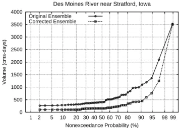
Fig. 2. Probability distribution forecasts from Des Moines River
en-semble streamflow prediction system for September 1965, with and without bias correction applied to the ensemble traces. The effect of bias correction is to shift the probability distribution forecasts.
The function fj()must be estimated using simulated and observed flows for a historical period. Let Yjibe the observed volume for month j in year i. Let ˜Yji be the model-simulated volume for month j in year i. Three methods are investigated for the function fj().
3.1 Event bias correction method
The event bias correction method, proposed by Smith et al. (1992), assumes that for a given historical weather sequence, the same multiplicative bias exists each time the sequence is used to simulate an ensemble trace, regardless of the initial conditions. Thus, the bias correction applied to ensemble volume ˆYjiis:
Zji = Bji · ˆYji (2) where Bji is the multiplicative bias associated with the weather sequence for month j and year i. Smith et al. (1992) estimate the multiplicative bias with observed and simulated flows from the historical record as:
Bji = Yji/ ˜Yji. (3) The unique feature of this method is that the multiplicative bias depends only on the weather sequence, and does not depend on the magnitude of the model-simulated ensemble volume. Note too that for the same simulated volume, the bias-corrected volume would be different for different input weather sequences. Hence, the bias-corrected volume is not a monotonic function of the simulated volume.
3.2 Regression method
The regression method removes bias by replacing the simu-lated volume with the expected value of the observed flow,
8000 6000 4000 2000 8000 6000 4000 2000 Observed volume (cms-days)
Simulated volume (cms-days)
September Monthly Volumes
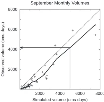
Fig. 3. Illustration of the LOWESS regression method. The crosses
show observed and simulated monthly flow volumes from the his-torical simulation. The solid line shows the LOWESS regression. The arrow illustrates the transformation of an ensemble trace to the bias-corrected ensemble trace.
given the simulated volume. Thus, the bias-correction trans-formation applied to ensemble volume ˆYji is:
Zji = E[Yji| ˆYji]. (4) A regression model, which is an estimate of this conditional expected value, is a natural choice for the transformation. The regression model is estimated using the observed and simulated flows from the historical record.
The regression technique known as LOWESS (LOcally WEighted Scatterplot Smoothing) was investigated for bias correction. Cleveland (1979) describes the LOWESS regres-sion technique in detail; we followed this approach, using the recommended PRESS (PRediction Error Sum of Squares) approach for estimating the smoothing parameter that de-termines the width of the moving window. In cases where this technique produced a local negative slope, the smooth-ing parameter was increased incrementally until a positive slope is obtained at all data points. This step ensures that the LOWESS regression produces a monotonic (one-to-one) relationship. Figure 3 shows an example of a LOWESS re-gression fitted to observed and simulated September monthly volumes from the historical simulation.
3.3 Quantile mapping method
The quantile mapping method uses the empirical probabil-ity distributions for observed and simulated flows to remove
biases. Let Foj be the cumulative distribution function of
the observed monthly volumes for month j . Let Fsj be the
cumulative distribution function of the corresponding sim-ulated flows from the historical simulation. The corrected ensemble volume is:
Zji = Fo−1
j (Fsj( ˆY i
j)). (5)
Figure 4 illustrates the concept of the transformation through a cumulative distribution function. In essence, this approach replaces the simulated ensemble volume with the observed flow that has the same nonexceedance probability. Instead of fitting a mathematical model to the cumulative distribu-tion funcdistribu-tions, we use a simple one-to-one mapping of or-der statistics of the observed and simulated monthly umes from the historical record. A corrected ensemble vol-ume is obtained from interpolation between the order statistic pairs. Note that similar approaches have been used by Leung et al. (1999), Wood et al. (2002), and others to correct biases in temperature and precipitation forecasts from atmospheric models for hydrologic forecasting.
4 Verification approach
We will use a forecast verification approach to assess the quality of the forecasts made using the bias-correction meth-ods. Verification compares forecasts with observed out-comes. Using the ensemble streamflow verification approach of Bradley et al. (2004), the ensemble is used to construct a set of probabilistic forecasts for flow occurrence events. Specifically, a flow threshold is chosen to define a discrete flow occurrence event. The event is said to occur if the ob-served monthly flow volume is below the threshold. The probabilistic forecast is then the probability of the event oc-currence, which is derived from the forecast cumulative dis-tribution function of ensemble volumes (Fig. 2). Let f de-note the probabilistic forecast, and let x dede-note the observed outcome. The binary outcome x is 0 if the flow volume is greater than the threshold, or 1 if the flow volume is less than or equal to the threshold; 0 indicates the event did not occur, and 1 means the event occurred.
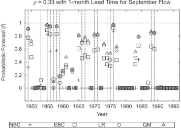
Figure 5 shows the probabilistic forecasts for September flow volume (1-month lead time) for a threshold defined by the 0.33 flow quantile (i.e., the flow corresponding to a nonexceedance probability p=0.33). Forecasts are shown for the system with no bias correction, as well as the fore-casts using the three bias correction methods. Event occur-rences (x=1) are indicated by the dashed vertical lines. Note that in most years when the event does not occur, the proba-bilistic forecasts for the event are near zero; when the event does occur, the probabilistic forecasts tend to be greater than zero.
For the evaluation of bias-correction methods, nine flow thresholds are defined, corresponding to the 0.05, 0.10, 0.25,
0 0.1 0.2 0.3 0.4 0.5 0.6 0.7 0.8 0.9 1 8000 6000 4000 2000 CDF
Observed volume (cms-days)
0 0.1 0.2 0.3 0.4 0.5 0.6 0.7 0.8 0.9 1 8000 6000 4000 2000
Simulated volume (cms-days)
September Monthly Volumes
Fig. 4. Illustration of the quantile mapping method. The panels show the empirical cumulative distribution function for the observed and
simulated monthly flow volume from the historical simulation. The arrows illustrate the transformation of an ensemble trace to the bias-corrected ensemble trace.
0.33, 0.50, 0.66, 0.75, 0.90, and 0.95 quantiles of the clima-tology of monthly volumes. The forecast-observation pairs for all the retrospective forecast dates create a verification data set. Summary measures of forecast quality are then computed using the verification data set constructed for in-dividual thresholds. We use distributions-oriented forecast verification techniques (Murphy, 1997) to assess the quality of the ensemble streamflow predictions. Measures derived from the joint distribution describe the various attributes. The measures presented in this study are described below. 4.1 Skill
The skill of the forecast is the accuracy relative to a reference forecast methodology. The mean square error (MSE) skill score using climatology as a reference (i.e., a forecast that is the climatological mean of the observation variable µx) is: SSMSE = 1 − [MSE/σx2], (6) where σx is the standard deviation of the observed stream-flow variable. For probabilistic forecasts, SSMSE is also known as the Brier skill score (Brier, 1950).
A skill score of 1 corresponds to perfect forecasts. For probabilistic forecasts, this means that the forecast probabil-ity f is always 1 when the event occurs (x=1), and always 0 when the event does not occur (x=0). A skill score of 0 means that the accuracy of the forecasts is the same as clima-tology forecasts (i.e., constant forecasts equal to the climato-logical mean µx). A skill of less than 0 means the accuracy is less than that of climatology forecasts. Therefore, forecasts where SSMSEis greater than 0 are skillful forecasts, and those where SSMSEis 0 or less have no skill.
0 0.2 0.4 0.6 0.8 1 1950 1955 1960 1965 1970 1975 1980 1985 1990 1995 Probabilistic Forecast ( )f Year
p = 0.33 with 1-month Lead Time for September Flow
NBC EBC LR QM
Fig. 5. Time series of probabilistic forecasts for event occurrences
from the ensemble streamflow predictions. The forecast event is for flow volume below the 0.33 quantile for September. The ver-tical dashed lines indicate years when the observed flow volume is below the quantile threshold. Probabilistic forecasts are shown for ensembles with no bias correction (NBC), and those bias corrected using event bias correction (EBC), LOWESS regression (LR), and quantile mapping (QM) methods.
4.2 Decomposition of skill
The MSE skill score can be decomposed as (Murphy and Winkler, 1992):
0 0.2 0.4 0.6 0.8 1 Dec Nov Oct Sep Aug Jul Jun May Apr Mar Feb Jan Simulated Month
Des Moines River at Stratford, Iowa
SS PS SREL SME
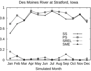
Fig. 6. Monthly variations in MSE skill score, and its
decomposi-tion, for the historical simulation of monthly flow volumes for the Des Moines River at Stratford. The plot shows the skill score (SS), the potential skill (PS), the slope reliability (SREL), and the stan-dardized mean error (SME).
where ρf x is the correlation of the forecasts and observa-tions, σf is the standard deviation of the forecasts, and µf and µx are the mean of the forecasts and the observations. The first term of the decomposition (right-hand side) is the potential skill of the forecasts (i.e., the skill if there were no biases). The second term is known as the slope reliability, and is a measure of the conditional bias. The third term is a standardized mean error, a measure of the unconditional bias. Expanding and rearranging the first two terms of the de-composition yields:
SSMSE = 2ρf x(σf/σx) − (σf/σx)2− [(µf − µx)/σx]2 (8) In this formulation of the skill score, the second term of the decomposition (right-hand side) is a measure of the sharp-ness of the forecasts. Sharp forecasts are ones where the forecast probabilities are close to 0 and 1. The first term is the product of the square roots of the potential skill and the sharpness, and is related to the discrimination of the fore-casts. Forecasts have discrimination when the forecasts is-sued for different outcomes (event occurrences or nonoccur-rences) are different. Hence, for forecasts to have good dis-crimination, they must both be sharp and have high poten-tial skill. Although other attributes of forecast quality (Mur-phy, 1997) were also assessed, the key aspects of the bias-correction methods will be illustrated using only the mea-sures described above.
5 Results
This section shows results of the diagnostic verification for monthly streamflow volume forecasts. First we examine the
skill of the simulation model and the ensemble predictions made at different times of the year, as well as the overall effect of the bias-correction methods. Next we explore the forecast quality characteristics of the probabilistic forecasts issued by the system for a critical period.
5.1 Historical simulation performance
Using the information in Table 1, the peformance of the cal-ibrated model in simulation mode can be reinterpreted in terms of the verification measures presented in Sect. 4. Fig-ure 6 shows the MSE skill score and its decomposition for the historical simulation of monthly volumes. The potential skill (PS) indicates that, without biases, the achievable skill of the hydrological model is high from April through September, and slightly lower from October through March. Indeed, the actual skill in simulation mode closely follows this pattern. The skill is reduced in the warm season due to unconditional biases (SME); the impact of unconditional bias is greatest in September. Conditional biases (SREL) also reduce the skill in the winter months; the impact on conditional bias is great-est in January. Overall, March and November are affected the least by conditional or unconditional biases.
5.2 Probabilistic forecast skill
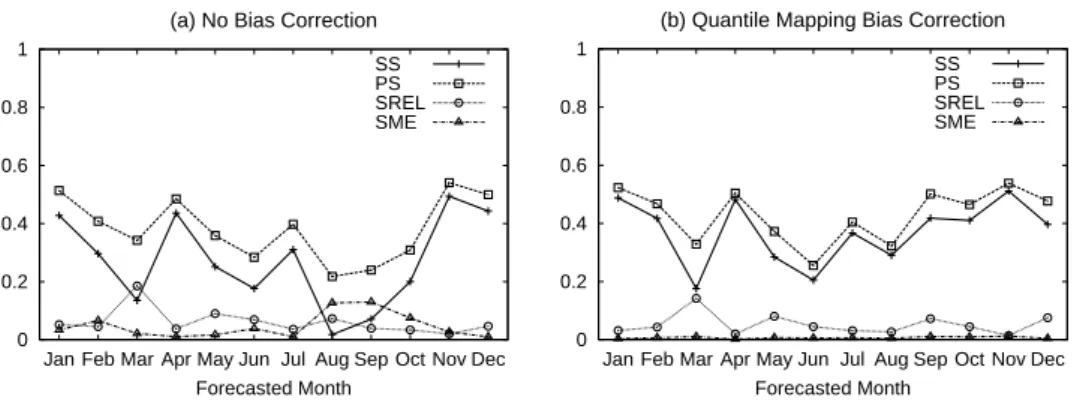
It seems logical to expect that in months where the simu-lation model performs well, its ensemble streamflow fore-casts would be good, and vice versa. However, this inference is incorrect for the experimental ensemble streamflow fore-casts. Figure 7a shows the average MSE skill score of the probability forecasts for the nine quantile thresholds. There is no strong correspondence with the skill in the historical simulation; the skill and potential skill are much more vari-able from month-to-month for the forecasts. Oddly, the high and low skill months are the opposite of those in the simu-lation mode; for the forecasts, the potential skill is higher in the cold season months, and is lower in the summer and fall months. Conditional and unconditional biases are present in all months, reducing the actual skill of the probabilistic fore-casts. For example, forecasts in August have almost no skill because of the biases. Several other months are noteworthy. September has the highest unconditional bias (SME) in sim-ulation mode (see Fig. 6); September also has relatively high unconditional and conditional bias for the probabilistic fore-casts (see Fig. 7a). However, January has the highest condi-tional bias (SREL) in simulation mode, but among the low-est conditional and unconditional biases for the probabilistic forecasts. And March has the lowest unconditional and con-ditional bias in simulation mode, but the highest concon-ditional biases for the probabilistic forecasts.
Clearly, the speculation that months with high relative ac-curacy or low biases in the historical simulation will have similar characteristics in their probabilistic forecasts is not true. Indeed, due to biases, some months have very little
0 0.2 0.4 0.6 0.8 1 Dec Nov Oct Sep Aug Jul Jun May Apr Mar Feb Jan Forecasted Month
(a) No Bias Correction
SS PS SREL SME 0 0.2 0.4 0.6 0.8 1 Dec Nov Oct Sep Aug Jul Jun May Apr Mar Feb Jan Forecasted Month
(b) Quantile Mapping Bias Correction
SS PS SREL SME
Fig. 7. Monthly variations in MSE Skill Score, and its decomposition, for 1-month lead-time probabilistic forecasts of monthly flow volumes
for the Des Moines River at Stratford with (a) no bias correction, and (b) quantile mapping bias correction. The plot shows the skill score (SS), the potential skill (PS), the slope reliability (SREL), and the standardized mean error (SME). The measures shown are the averages over all nine thresholds for which the probabilistic forecasts were issued.
probabilistic forecast skill, despite having good skill in sim-ulation mode.
5.3 Effect of bias correction
Figure 7b shows how bias correction changes the MSE skill and its decompositions for the probabilistic forecasts. The results shown are using the quantile mapping approach, but conclusions are similar for all approaches. For the proba-bilistic forecasts, the unconditional biases (SME) are nearly eliminated; however, no significant reductions in the condi-tional biases (SREL) occur with bias correction.
The effects of all three bias-correction methods are seen in Fig. 8. Although all the bias-correction methods applied to the ensemble volumes improve the skill in most months, no one method is clearly superior. The improvements by the bias-correction methods also vary by month, correspond-ing to the magnitude of the unconditional bias. Overall, the experimental forecast system produces skillful probabilistic forecasts for all months when bias correction is applied to ensemble traces. However, without bias correction, the Au-gust and September monthly volume forecasts have almost no skill.
The statistical significance of the skill scores can be eval-uated using a bootstrap resampling approach (for example, see Zhang and Casey, 2000). For the small sample sizes used (N =48), the computed skill scores have large sampling un-certainties. For example, if the climatology forecasts from the original sample were issued for a randomly selected sam-ple of 48 events, a samsam-ple skill score of 0.237 or greater would occur 5% of the time by chance, even though by def-inition, the true skill of climatology forecasts is zero. Using this level (Fig. 8) as an indication of statistical significance, we can conclude that the average skill score is statistically significant in most months. However, in May and June, one cannot reject a hypothesis of zero skill for the forecasts, with or without bias correction. During the months from August
0 0.2 0.4 0.6 0.8 1 Dec Nov Oct Sep Aug Jul Jun May Apr Mar Feb Jan
MSE Skill Score
Forecasted Month
Probabilistic Forecasts with 1-month lead time NBC
EBC LR QM
Fig. 8. The effect of bias correction on the monthly variations in
MSE skill score for 1-month lead-time probabilistic forecasts of monthly flow volumes for the Des Moines River at Stratford. Re-sults are shown for probabilistic forecasts with no bias correction (NBC), and those bias corrected using event bias correction (EBC), LOWESS regression (LR), and quantile mapping (QM) methods. The measure shown is the average skill score over all nine thresh-olds for which the probabilistic forecasts were issued. Skill scores greater than 0.237 (dashed horizontal line) are significantly differ-ent from zero-skill climatology forecasts at the 5% level.
to October, the forecasts with bias correction have statisti-cally significant skill, whereas those without bias correction do not.
5.4 Probabilistic forecast skill and lead time
For months with significant unconditional biases, implemen-tation of bias-correction methods is critical for long-lead probabilistic forecasts. As an example, September monthly volume forecasts have no skill at 2-month lead times or
-0.2 -0.1 0 0.1 0.2 0.3 0.4 0.5 0.6 1 2 3 4 5 6
MSE Skill Score
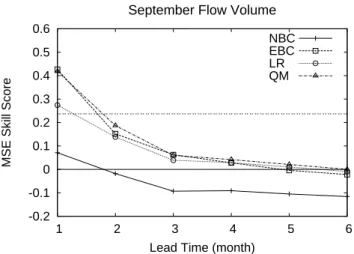
Lead Time (month) September Flow Volume
NBC EBC LR QM
Fig. 9. Variations by lead time in MSE skill score for the probabilistic forecasts of September monthly flow volumes. Re-sults are shown for probabilistic forecasts with no bias correction (NBC), and those bias corrected using event bias correction (EBC), LOWESS regression (LR), and quantile mapping (QM) methods. The measure shown is the average skill score over all nine thresh-olds for which the probabilistic forecasts were issued. Skill scores greater than 0.237 (dashed horizontal line) are significantly differ-ent from zero-skill climatology forecasts at the 5% level.
longer without bias correction (Fig. 9). Bias correction us-ing any of the three methods removes the unconditional bi-ases, producing skillful probabilistic forecasts for longer lead times. However, due to the small sample sizes, the skill scores are statistically significant only for a 1-month lead time. Similar to the results for September, the probabilistic forecasts made in other months (not shown) lose virtually all their skill at lead times of a few months. However, the rate of decrease depends on the month. Ironically, in the warm sea-son, where the historical simulation performance is best, the skills drops off quickly; in the cold season, where the simu-lation performance is poorer, the rate of decrease is slower.
We also examined the variations in probabilistic forecast bias with lead time (not shown). For a given approach (with or without bias correction), the probabilistic forecast bias is virtually the same at all lead times. This result is not surpris-ing, given that the retrospective forecasts are initialized us-ing the model-simulated moisture states on the forecast date from the continuous simulation. However, variations with lead time might be significant if moisture states are adjusted in real-time by a forecaster or with a data assimilation sys-tem.
5.5 Skill decomposition for September
Since the bias-correction methods produce dramatic im-provements for the September forecasts, we examine the quality of the probabilistic forecasts for each of the nine quantile thresholds in detail in Fig. 10. Note that the skill is not the same for all quantile thresholds. Without bias
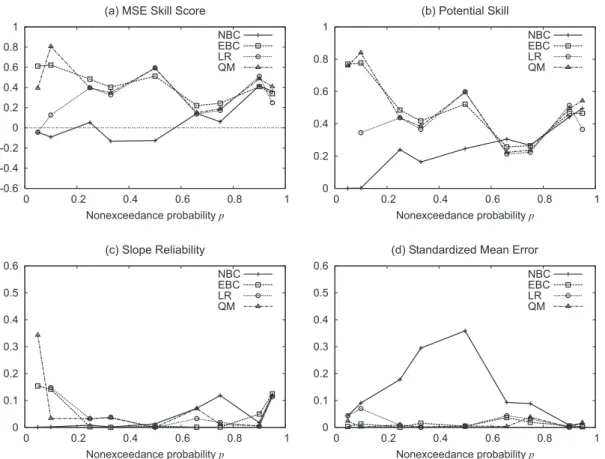
cor-rection (NBC), the skill is at or below climatology for prob-abilistic forecasts of low to moderate flow events (Fig. 10a). In contrast, all the bias-correction methods significantly im-proved the skill for low to moderate events, and as a re-sult, the skill for low to moderate flow events is generally greater than that for high flow events. An exception is the 0.05 and 0.10 quantile threshold for the LOWESS regres-sion method (LR), where the skill is much lower than for the other two bias-correction methods. At higher levels, quan-tile mapping (QM) and LOWESS regression methods have similar patterns. Both are monotonic transformations of sim-ulated flows; the transformations are fairly similar expect for low flows, which do not appear to be well represented by the LOWESS regression. In contrast, the event bias correction (EBC) is not a monotonic transformation, so its pattern dif-fers from the other methods.
Examining the skill score decomposition in Eq. (7), the improvement in probabilistic forecast skill from bias correc-tion comes from two sources. Not surprisingly, one comes from the elimination of unconditional biases (SME), espe-cially for moderate thresholds. However, it is surprising that all the bias-correction methods also improve the potential skill (PS) for low to moderate thresholds. The third com-ponent, the conditional biases (SREL) are relatively low for September without bias correction; for some thresholds, bias correction actually increases the conditional biases some-what.
Although the various bias-correction methods are similar in terms of probabilistic forecast skill for most thresholds, there are subtle differences in the nature of the forecasts. In particular, the sharpness of the probabilistic forecasts differ for the bias-correction methods (Fig. 11). Except for the lowest quantile thresholds, the quantile mapping (QM) and LOWESS regression (LR) methods produce sharper fore-cast than those for the event bias correction (EBC) method. Sharper forecasts have event forecast probabilities closer to 0 or 1. The sharper forecasts also have higher discrimina-tion, since the potential skill is similar for each method. The higher discrimination for the quantile mapping and LOWESS regression methods means that event occurrences (nonoccur-rences) or more common when the forecast probability is high (low).
5.6 Prototype decision problem
The impact of these differences in the nature of the forecasts can be understood using a simple prototype decision prob-lem. Suppose that a decision-maker uses a September fore-cast of the probability of a low-flow event, assumed here to be defined by the 0.33 quantile threshold, to initiate some action. If the forecast probability exceeds a specified thresh-old probability, action is initiated; if the forecast probabil-ity is less than the threshold probabilprobabil-ity, no action is taken. Here we will compare the use of forecasts for the 0.33 quan-tile low-flow event made using event bias correction (EBC),
-0.6 -0.4 -0.2 0 0.2 0.4 0.6 0.8 1 0 0.2 0.4 0.6 0.8 1 Nonexceedance probability p (a) MSE Skill Score
NBC EBC LR QM 0 0.2 0.4 0.6 0.8 1 0 0.2 0.4 0.6 0.8 1 Nonexceedance probability p (b) Potential Skill NBC EBC LR QM 0 0.1 0.2 0.3 0.4 0.5 0.6 0 0.2 0.4 0.6 0.8 1 Nonexceedance probability p (c) Slope Reliability NBC EBC LR QM 0 0.1 0.2 0.3 0.4 0.5 0.6 0 0.2 0.4 0.6 0.8 1 Nonexceedance probability p (d) Standardized Mean Error
NBC EBC LR QM
Fig. 10. Variations over the thresholds in MSE skill score, and its decomposition, for 1-month lead-time probabilistic forecasts of September
monthly volumes. The panel shows (a) the MSE skill score, (b) the potential skill, (c) the slope reliability, and (d) the standardized mean error. Results are shown for probabilistic forecasts with no bias correction (NBC), and those bias corrected using event bias correction (EBC), LOWESS regression (LR), and quantile mapping (QM) methods.
which have slightly higher skill (see Fig. 10a), with those made using the quantile mapping (QM) mapping approach, which are sharper (Fig. 11).
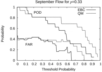
In selecting a threshold probability to initiate action, the decision-maker wants the probability of detection (POD) for the event occurrence to be high. That is, when an event ac-tually occurs, the forecast probability is high enough that the decision-maker initiates action. On the other hand, the false-alarm ratio (FAR) for the event should be low. That is, when the decision-maker initiates action, the event usually occurs (e.g., low flows). The probability of detection and the false-alarm ratio over the range of possible threshold probabilities for initiating action are shown in Fig. 12. Note that if the threshold probability is relatively low, the forecasts for both methods have high probability of detection, but the false-alarm ratio is also high. Yet at higher thresholds, the fore-cast made using the quantile mapping (QM) bias-correction method have a much higher probability of detection, but also a higher false-alarm ratio.
The trade-off between the probability of detection and the false-alarm ratio over the range of threshold probabilities is
known as the relative operating characteristics (Wilks, 1995), and is shown in Fig. 13. Since the ideal situation would be to choose a threshold probability threshold with high proba-bility of detection (POD) and low false-alarm ratio (FAR), combinations close to the upper left portion are superior. Note that the relative operating characteristics for the quan-tile mapping (QM) forecasts are as good, or superior to those, for the event bias correction (EBC) forecasts. Hence, given the costs and losses associated with false alarms and non-detection, a decision-maker might have a strong preference for using the quantile mapping forecasts (with an appropri-ately selected threshold probability for action), despite the fact that the event bias correction forecasts are slightly more skillful for this threshold.
6 Summary and conclusions
Three different bias-correction methods were used to adjust ensemble streamflow volume traces for the Des Moines River at Stratford, Iowa, USA. The event bias correction applies a multiplicative bias to the simulated volume trace based on the
0 0.2 0.4 0.6 0.8 1 1.2 0 0.2 0.4 0.6 0.8 1 Relative Sharpness Nonexceedance probability p
September Flow with 1-month Lead Time (N=48) NBC
EBC LR QM
Fig. 11. Variations in the relative sharpness for 1-month lead-time
probabilistic forecasts of September monthly volumes. Results are shown for forecasts with no bias correction (NBC), and those cor-rected using the event bias correction (EBC), LOWESS regression (LR), and quantile mapping (QM) methods.
0 0.2 0.4 0.6 0.8 1 0 0.1 0.2 0.3 0.4 0.5 0.6 0.7 0.8 0.9 1 Probability Threshold Probability September Flow for p=0.33 POD
FAR
EBC QM
Fig. 12. Probability of detection (POD) and false-alarm ratio (FAR)
for forecasts of a low-flow event occurrence using event bias correc-tion (EBC) and quantile mapping (QM) bias correccorrec-tion. The low-flow event is defined by the 0.33 quantile of September monthly flow volume. The threshold probability is the forecast probability for the event used for decision-making.
input weather sequence; the bias is assumed to be the same as observed with the weather sequence in a historical ulation of flows. The regression method replaces the sim-ulated volume trace with its conditional expected volume, developed using a LOWESS regression technique. The re-gression is obtained using simulated and observed volumes from a historical simulation. The quantile mapping method adjusts an ensemble volume based on the historical cumula-tive distribution of simulated and observed flows, so that the
0 0.2 0.4 0.6 0.8 1 0 0.2 0.4 0.6 0.8 1 POD FAR
September Flow for p=0.33
EBC QM
Fig. 13. The relative operating characteristics for forecasts of a
low-flow event occurrence using event bias correction (EBC) and quan-tile mapping (QM) bias correction. The low-flow event is defined by the 0.33 quantile of September monthly flow volume. The re-sults show the trade-off between the probability of detection (POD) and the false-alarm ratio (FAR) over the entire range of threshold probabilities for decision-making (see Fig. 12).
simulated and corrected trace volume have the same nonex-ceedance probability.
A distribution-oriented approach was used to assess the quality of ensemble streamflow forecasts made with and without bias correction. Interestingly, situations where the hydrologic model performed better in calibration and valida-tion simulavalida-tions did not translate into better skill in forecast-ing. In fact, months where probabilistic streamflow forecasts had the greatest skill were months where the model demon-strated the least skill in simulation. This result shows that the forecast quality of a hydrologic model should not be inferred from its performance in a simulation mode.
In terms of forecast skill, all three bias-correction meth-ods performed well for monthly volume forecasts. Since both the regression and the quantile mapping methods em-ploy a monotonic transformation of a simulated trace vol-ume, both produce similar results. The exception was for low flows, where the regression method performed poorly due to its model fit. Although alternate regression formu-lations could be used with the regression method, the sim-plicity of the quantile mapping may favor its selection for applications. The forecast skill for the event bias correction method is similar to the others, but the sharpness and dis-crimination of the probabilistic forecasts are less. As demon-strated using a simple prototype decision problem, this differ-ence can be significant for use of the bias-corrected forecasts in decision-making. This example shows that distributions-oriented forecast verification usefully quantifies and distin-guishes the aspects of forecast quality that are meaningful in decision-making, providing criteria to choose among bias-correction techniques with comparable skill.
The decomposition of the skill scores reveal that all the bias-correction methods achieve better skill by reducing the unconditional bias and increasing the potential skill of prob-abilistic forecasts. However, bias correction does not re-duce the conditional biases. Another way of implementing bias correction is to directly adjust the probability distribu-tion forecast based on the original ensemble traces, rather than adjusting each model-simulated trace independently. Such a post-hoc correction developed using a verification data set is often referred to as calibration. Several cali-bration methods include the use of the conditional mean given the forecast (Atger, 2003), the use of a linear regres-sion between probability forecasts and observations (Stew-art and Reagan-Cirincione, 1991; Wilks, 2000), or more so-phisticated approaches using the rank histogram (Hamill and Colucci, 1997). An advantage of post-hoc calibration is that it can minimize both unconditional and conditional bi-ases. Given that the unconditional biases remained with the trace-adjustment bias-correction methods, additional im-provements may be possible using a calibration technique. Investigation is needed to compare the different approaches; if post-hoc calibration is superior, techniques for using the results to adjust individual traces may still be needed in plications where the traces are utilized in water resources ap-plications.
In this study, we focused only on the bias correction for monthly flow volumes. Yet in many applications, ensemble traces at daily or weekly time scales are needed. Clearly, bias correction for weekly or daily flows will be more com-plex. Correcting each time period separately, using tech-niques similar to those present here, ignores the autocorrela-tion of simulaautocorrela-tion errors for daily and weekly flows. Clearly, there is a need for additional study to develop and evalu-ate more sophisticevalu-ated approaches for bias correction of en-semble streamflow predictions for applications at finer time scales.
Acknowledgements. This work was supported in part by Na-tional Oceanic and Atmospheric Administration (NOAA) grant #NA16GP1569, from the Office of Global Programs as part of the GEWEX Americas Prediction Project (GAPP), and grant #NA04NWS4620015, from the National Weather Service (NWS) Office of Hydrologic Development. We gratefully acknowledge this support. We would also like to thank an anonymous reviewer for constructive comments on this paper.
Edited by: R. Rudari
References
Atger, F.: Spatial and interannual variability of the reliability of ensemble-based probabilistic forecasts: consequences for cali-bration, Mon. Wea. Rev., 131, 1509–1523, 2003.
Bicknell, B., Imhoff, J., Kittle Jr., J. L., Donigian Jr., A. S., and Jo-hanson, R. C.: Hydrological Simulation Program – FORTRAN: User’s Manual for Version 11, Tech. Rep. EPA/600/R-97/080,
U.S. Environmental Protection Agency, National Exposure Re-search Laboratory, 1997.
Bradley, A. A., Hashino, T., and Schwartz, S. S.: Distributions-oriented verification of ensemble streamflow predictions, J. Hy-drometeorol., 5, 532–545, 2004.
Brier, G. W.: Verification of forecasts expressed in terms of proba-bility, Mon. Wea. Rev., 78, 1–3, 1950.
Carpenter, T. M. and Georgakakos, K. P.: Assessment of Folsom lake response to historical and potential future climate scenarios: 1. Forecasting, J. Hydrol., 249, 148–175, 2001.
Clark, M. P. and Hay, L. E.: Use of medium-range numerical weather prediction model output to produce forecasts of stream-flow, J. Hydrometeorol., 5, 15–32, 2004.
Cleveland, W.: Robust locally weighted regression and smoothing scatterplots, J. Amer. Stat. Assoc., 74, 829–839, 1979.
Connelly, B., Braatz, D. T., Halquist, J. B., DeWeese, M., Larson, L., and Ingram, J. J.: Advanced hydrologic prediction system, J. Geophys. Res.-Atmos., 104, 19 655–19 660, 1999.
Day, G. N.: Extended streamflow forecasting using NWS-RFS, J. Water Resour. Planning Manage., 111, 157–170, 1985.
Donigian, A. S., J., Imhoff, J., Bicknell, B., and Kittle, J. L.: Appli-cation Guide for Hydrological Simulation Program-FORTRAN, Tech. Rep. EPA-600/3-84-065, U.S. Environmental Protection Agency, Environ. Res. Laboratory, 1984.
Duan, Q. Y., Sorooshian, S., and Gupta, V.: Effective and efficient global optimization for conceptual rainfall-runoff models, Water Resour. Res., 28, 1015–1031, 1992.
Faber, B. A. and Stedinger, J. R.: Reservoir optimization using sam-pling SDP with ensemble streamflow prediction (ESP) forecasts, J. Hydrol., 249, 113–133, 2001.
Franz, K. J., Hartmann, H. C., Sorooshian, S., and Bales, R.: Veri-fication of national weather service ensemble streamflow predic-tions for water supply forecasting in the Colorado River basin, J. Hydrometeorol., 4, 1105–1118, 2003.
Georgakakos, A. P., Yao, H. M., Mullusky, M. G., and Georgakakos, K. P.: Impacts of climate variability on the operational forecast and management of the upper Des Moines River basin, Water Resour. Res., 34, 799–821, 1998.
Grantz, K., Rajagopalan, B., Clark, M., and Zagona, E.: A tech-nique for incorporating large-scale climate information in basin-scale ensemble streamflow forecasts, Water Resour. Res., 41, W10 410, doi:10.1029/2004WR003467, 2005.
Hamill, T. M. and Colucci, S. J.: Verification of Eta-RSM short-range ensemble forecasts, Mon. Wea. Rev., 125, 1312–1327, 1997.
Hamlet, A. F. and Lettenmaier, D. P.: Columbia River streamflow forecasting based on ENSO and PDO climate signals, J. Water Resour. Planning Manage.-Asce, 125, 333–341, 1999.
Hamlet, A. F., Huppert, D., and Lettenmaier, D. P.: Economic value of long-lead streamflow forecasts for Columbia River hy-dropower, J. Water Resour. Planning and Management-Asce, 128, 91–101, 2002.
Hashino, T., Bradley, A. A., and Schwartz, S. S.: Verification of Probabilistic Streamflow Forecasts, Tech. Rep. IIHR Report No. 427, IIHR-Hydrosci. Eng., 2002.
Kim, Y. O., Jeong, D. I., and Kim, H. S.: Improving water sup-ply outlook in Korea with ensemble streamflow prediction, Water Int., 26, 563–568, 2001.
Simulations of the ENSO hydroclimate signals in the Pacific Northwest Columbia River basin, Bull. Amer. Meteorol. Soc., 80, 2313–2328, 1999.
McEnery, J., Ingram, J., Duan, Q. Y., Adams, T., and Anderson, L.: NOAA’s advanced hydrologic prediction service – Building pathways for better science in water forecasting, Bull. Amer. Me-teorol. Soc., 86, 375–385, 2005.
Murphy, A. H.: Forecast Verification, in: Economic Value of Weather and Climate Forecasts, edited by: Katz, R. W. and Mur-phy, A. H., p. 19–74, Cambridge University, New York, 1997. Murphy, A. H. and Winkler, R. L.: A general framework for forecast
verification, Mon. Wea. Rev., 115, 1330–1338, 1987.
Murphy, A. H. and Winkler, R. L.: Diagnostic verification of prob-ability forecasts, Int. J. Forecasting, 7, 435–455, 1992.
Roulin, E. and Vannitsem, S.: Skill of medium-range hydrological ensemble predictions, J. Hydrometeorol., 6, 729–744, 2005. Smith, J. A., Day, G. N., and Kane, M. D.: Nonparametric
frame-work for long-range streamflow forecasting, J. Water Resour. Planning and Management, 118, 82–91, 1992.
Souza Filho, F. A. and Lall, U.: Seasonal to interannual ensemble streamflow forecasts for Ceara, Brazil: Applications of a multi-variate, semiparametric algorithm, Water Resour. Res., 39, 1307, doi:10.1029/2002WR001373, 2003.
Stewart, T. R. and Reagan-Cirincione, P.: Coefficients for debiasing forecasts, Mon. Wea. Rev., 119, 2047–2051, 1991.
Wilks, D. S.: Statistical Methods in the Atmospheric Science, Aca-demic Press, New York, 1995.
Wilks, D. S.: Diagnostic verification of the Climate Prediction Cen-ter Long-Lead Outlooks, 1995–98, J. Climate, 13, 2389–2403, 2000.
Wood, A. W., Maurer, E. P., Kumar, A., and Lettenmaier, D. P.: Long-range experimental hydrologic forecasting for the eastern United States, J. Geophys. Res.-Atmos., 107, 4429, doi:10.1029/2001JD000659, 2002.
Yao, H. and Georgakakos, A.: Assessment of Folsom Lake response to historical and potential future climate scenarios 2. Reservoir management, J. Hydrol., 249, 176–196, 2001.
Zhang, H. and Casey, T.: Verification of categorical probability forecasts, Weather and Forecasting, 15, 80–89, 2000.
![[PDF] Cours general des nouveautés de Lua | Cours informatique](data:image/gif;base64,R0lGODlhAQABAIAAAP///wAAACH5BAEAAAAALAAAAAABAAEAAAICRAEAOw==)