HAL Id: hal-01221709
https://hal.archives-ouvertes.fr/hal-01221709
Submitted on 16 Apr 2021
HAL is a multi-disciplinary open access archive for the deposit and dissemination of sci-entific research documents, whether they are pub-lished or not. The documents may come from teaching and research institutions in France or abroad, or from public or private research centers.
L’archive ouverte pluridisciplinaire HAL, est destinée au dépôt et à la diffusion de documents scientifiques de niveau recherche, publiés ou non, émanant des établissements d’enseignement et de recherche français ou étrangers, des laboratoires publics ou privés.
Adaptive zooming method for the analysis of large
structures with localized nonlinearities
Antoine Llau, Ludovic Jason, Frédéric Dufour, Julien Baroth
To cite this version:
Antoine Llau, Ludovic Jason, Frédéric Dufour, Julien Baroth. Adaptive zooming method for the analysis of large structures with localized nonlinearities. Finite Elements in Analysis and Design, 2015, 106, pp.73-84. �10.1016/j.finel.2015.07.011�. �hal-01221709�
1
Adaptive zooming method for the analysis of large structures with
localized nonlinearities
Antoine Llau a,b,*, Ludovic Jason a,d, Frédéric Dufour b,c, Julien Baroth b,c a CEA, DEN,DANS,DM2S,SEMT,LM2S, 91191 Gif-sur-Yvette Cedex, France b Univ. Grenoble Alpes, 3SR, 38000 Grenoble, France
c CNRS, 3SR, 38000 Grenoble, France
d IMSIA, UMR 9219 CNRS-EDF-CEA-ENSTA, Université Paris Saclay, 91762 Palaiseau Cedex, France
* Corresponding author: CEA,DEN,DANS,DM2S,SEMT,LM2S, 91191 Gif-sur-Yvette Cedex, France
[email protected], +33 (0)169088747
Abstract
Simulating concrete cracking requires nonlinear modelling applied on a refined mesh if a correct evaluation of crack properties needs to be achieved. Therefore, it is rather costly and even sometimes impossible when large reinforced concrete structures are considered. Alternative
solutions have therefore to be proposed. This contribution presents a structural zooming method for the simulation of large reinforced concrete structures with localized nonlinearities. Our method is based on static condensation (Guyan 1965,[1]) and provides an adaptive framework for
performance-oriented use of this method in nonlinear simulations. In particular, it only simulates the behavior of nonlinear interesting zones (detected by adapted criteria). The areas where refined modelling is not required are replaced by their equivalent stiffnesses. The linearity criteria,
depending on the chosen mechanical models, are also used to activate new interesting zones during the simulation. This method substantially decreases the computational cost on both presented test cases (a two-dimensional concrete beam and a three-dimensional reinforced concrete building).
Keywords
Structural zooming, Static condensation, Concrete cracking, Reduced-order modelling.
1 Introduction
With recent improvements in numerical and behavior models and new features of simulation software, the complexity of models used by physicists and engineers is rising. Scalability of models and computations has become a key issue, as simulation of local small-scale phenomenon on large-scale problems seems to be the next frontier in computing. The interaction between different large-scales and different physics raises new questions, such as the localization and quantification of cracking risk (civil engineering, aeronautics …).
In this contribution, the specific physical phenomenon to be predicted is the cracking of large-scale concrete and reinforced concrete structures. A damage mechanics approach is used to model the behavior of concrete with the finite elements method. Simulating this phenomenon requires refined nonlinear models of the behavior of concrete (for instance, a damage mechanics approach), applied on meshes fine enough to match the physical phenomena. Those models are hardly applicable to large-scale civil engineering structures with a mesh fine enough to adequately represent cracking.
2
However, concrete cracking is a phenomenon that is localized on large structures, and therefore, realizing a fully refined simulation of a large structure is unnecessary to obtain data on cracking: A method for simulating localized nonlinearities on large problems with accurate local information is required. Several techniques bring answers to this scalability need.
For instance, global-local analysis methods are mainly used in multi-scale simulations where physical phenomena appear at different scales of the problem. They allow separating the scales and therefore limit the complexity of the global problem [2]. These methods combine a coarse simulation at the large scale and a fine simulation at the small scale. Boundary conditions are exchanged between both simulations and an iterative scheme allows finding a solution satisfying both scales. Separating scales however requires the definition of a REV (Representative Elementary Volume), small enough to be considered as representative of the material behavior seen as homogenous at the large scale and large enough to represent a mean behavior at the small scale. To our knowledge, the definition of a REV for a cracked material is still under discussion. Also some variations on this methodology exist [3–6], eventually combining different models but also different numerical methods, such as Confinement-Shear-Lattice [7] or discrete elements [8]. A zooming method using global-local methodology has been introduced in 2003 by Haidar et al. to simulate cracking of concrete [9]. Another approach to solve large structural problems in limited computation time is the use of parallel computing and domain decomposition method, that decompose a large problem in smaller subproblems solved independently [10,11]. Those methods divide the computing load to take advantage of parallel architectures and solve problems faster. However, they do not affect the global computing load, and will not allow finer simulations for a given computing power [12–14].
Model reduction methods, and zooming method which derived from them, are used when complex phenomena operate in a localized manner on a large dimension problem. These methods aim to simplify at most the modelling of the areas that present no complex phenomenon, and focus the computational effort where it is the most necessary, to limit the global computing load [15]. One of the most widely used model reduction technique is orthogonal decomposition, e.g. using Karhunen-Loève expansion. It was introduced in structural mechanics by Spanos and Ghanem, based on the method previously used in fluid [16–18]. It consists in analyzing by the method of principal
component analysis the mechanical responses depending on solicitations and parameters to build a predictive model. Applying this technique to a substructure allows to replace its model by a
linearized model and focuses the computational effort on other substructures [19]. Possible applications include fluid mechanics, shape optimization, nuclear structure dynamic analysis [20], and stochastic structural simulation with finite elements [21]. However, those methods require previous knowledge on the localization of nonlinearities (and specifically the cracks in concrete) and are unable to detect the appearance of new cracks out of the zoomed areas.
The static condensation method, or superelements method, was introduced by Guyan [1]. It simplifies the solving of large-scale linear problems by eliminating a well-chosen subsystem of degrees of freedom. Several developments have been made on the static condensation method, such as adaptation to dynamic problems. Dynamic condensation was introduced to reduce computational cost of the dynamical analysis of large structures [15,22]. Applications are found in various fields, such as earthquake engineering, or vehicle suspension-tires systems simulation [23].
3
The first structural zooming method was introduced by Hirai et al. [24,25]. It combines static condensation with the reanalysis methods introduced by Wang and Pilkey [26] and remeshing techniques to locally improve the quality of numerical simulation. Starting with a relatively coarse mesh, it can be locally refined (on a substructure) with a remeshing technique. A new stiffness is calculated with the new mesh (and degrees of freedom) on the substructure, which is then
condensed on the coarse mesh by Guyan reduction, and reintroduced in the global problem. Solving the problem gives the condensed solution on the original mesh, and the local subproblem can be solved from there. Only the stiffness of the area of interest is then condensed in this method. This method can also be used to combine different models at different scales, such as beam theory with nonlinear mechanics in aeronautical structural mechanics [27].
Several of the previously cited methods allow limiting the computational cost on problems similar to the cracking prediction on large concrete structures. However, all focus on obtaining the correct global behavior for the structure. Since an accurate simulation of the cracked areas is required, a new method has been developed, that focuses the computational effort on the local simulation. The proposed structural zooming method aims at reproducing at the local scale the results of a full nonlinear simulation for a fraction of the computation cost. This adaptive structural zooming method is presented in section 2. Finally, the method is applied to a bending concrete beam and a reinforced concrete building under pressure.
2 Structural zooming method
2.1 Guyan condensation method: General principle
This paragraph describes the first-level Guyan reduction technique used in this zooming method for structural mechanics. The discretized problem of continuum mechanics to be solved at each area is formulated as follows:
KU F (1)
In the field of mechanics, with 𝑛 degrees of freedom, 𝐾 represents the structural stiffness matrix (𝐾 ∈ ℝ𝑛,𝑛), 𝑈 the nodal displacement (𝑈 ∈ ℝ𝑛), and 𝐹 the equivalent external nodal force vector (𝐹 ∈ ℝ𝑛). All stiffness matrices are supposed invertible, that simplifies the formulation, and
computational methods allow bringing properly-formulated problems back to this case. In particular, in the simulation software used in this study, Cast3M [28], boundary conditions are treated using the double Lagrange multiplier method: This method allows to keep invertible stiffness matrices that contains the boundary conditions (of the form 𝐶𝑈𝑖 = 𝑈𝑑) if the Lagrange multiplier vectors are added to the degrees of freedom 𝑈 of the system [29].
By using two subdomains (𝑠 and 𝑚), the system becomes:
, , , ,
,
,
s s s m s s m s m m m mK
K
F
U
F
U
K
K
K
F
U
(2)4
with 𝐹s, 𝑈𝑠 ∈ ℝ𝑝, 𝐹𝑚, 𝑈𝑚 ∈ ℝ𝑞, 𝐾𝑠,𝑠 ∈ ℝ𝑝,𝑝, K𝑠,𝑚∈ ℝ𝑝,𝑞, 𝐾𝑚,𝑠∈ ℝ𝑞,𝑝, 𝐾𝑚,𝑚∈ ℝ𝑞,𝑞 , 𝑛 = 𝑝 + 𝑞. The system is rewritten to solve the equation of the 𝑚 subdomain, using the “condensed”, or “equivalent stiffness” 𝐾̂ of both subdomains [1]:
1 ,
(
,)
s s s s s m mU
K
F
K U
(3)ˆ
ˆ
mKU
F
(4) 1 , , , , 1 , ,ˆ
ˆ
m m m s s s s m m m s s s s
K
K
K
K K
F
F
K
K F
(5)Eq. (4) is called the condensed problem. Considered independently, this 𝑞-dimensional condensed problem (𝑞 < 𝑛) is simplified and therefore faster to solve than the initial 𝑛-dimensional system. It solves the problem for subdomain m, and its result allows deducing the solution for subdomain s from eq. (3). A term of “equivalent loading” (−𝐾𝑚,𝑠𝐾𝑠,𝑠−1𝐹𝑠) appears in the condensed problem (eq. 5). It contains the influence of the external forces 𝐹𝑠 applied on the 𝑠 subdomain over the 𝑚
subdomain: The subdomains have therefore been decoupled in terms of degrees of freedom but not in terms of forces and stiffnesses.
2.2 Proposed approach
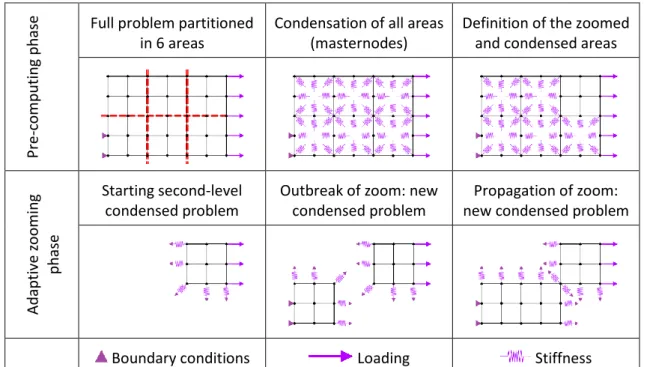
This method provides a framework for an adaptive, local-scale oriented use of a two-level Guyan condensation method when solving nonlinear structural problems. It follows several steps. Figure 1 describes the different steps of the method applied to a 2D plate problem decomposed in 6 areas. It illustrates the general principle of the method on a small academic problem. Two phases can be distinguished: a pre-computing phase and an adaptive zooming phase, which takes place during the simulation. P re -c o m p u tin g ph
ase Full problem partitioned in 6 areas
Condensation of all areas (masternodes)
Definition of the zoomed and condensed areas
Ad ap tiv e zo o m in g p h ase Starting second-level condensed problem
Outbreak of zoom: new condensed problem
Propagation of zoom: new condensed problem
Boundary conditions Loading Stiffness
5 2.2.1 Pre-computing and zoom initiation 2.2.1.1 Partitioning of the problem
The structural problem is first partitioned in 𝑁 subdomains: Each of these areas will either be zoomed or condensed depending on the expected behavior. The problem decomposition in
subproblems is the most critical parameter for the structural zooming method’s performance. It has no impact on the results of the simulation, but it is critical for the computational load. This
decomposition defines directly the dimension of the problem solved at each increment: the number and shape of the areas define which part of the model is zoomed during the simulation. The closer the area decomposition matches the nonlinearities localization and their evolution in the structure, the most efficient the zooming method will be. For instance, with only one area, the full structure is systematically zoomed: this implies a null gain in computational load compared to a standard simulation. On the other hand, a model dividing the nonlinear areas in a very large number of substructures would require more updates when nonlinearities would spread, hence a large
computation cost during the adaptive zooming phase. The decomposition must then be the result of a compromise between model size and update frequency, and match as close as possible the areas where nonlinear behavior is expected.
This approach, with fixed subdomains has been chosen instead of flexible areas following nonlinearities and dynamically reshaping (as in other methods of structural zooming) because it presents several advantages:
The equivalent stiffness of each zone only needs to be computed once: the cost of computing and inverting stiffness matrices is then reduced.
The interface between the areas only needs to be determined once, before the simulation. However, its main drawback is the dependency of the computational performance on the area decomposition: the method will be as efficient to reduce computational load as the shape of the zoomed areas is able to match the damaged part of the structure through the loading.
2.2.1.2 Condensation of each area on its boundaries
Using the Guyan reduction technique described, each area is condensed on its boundaries: the equivalent stiffness and equivalent loading are calculated (and will be useful during the simulation). It is to be noted that the equivalent stiffness of each area takes into account the material stiffnesses, the additional stiffnesses (multi-material adhesion, etc.), and the boundary conditions applied to the area. It is to be noted that only force-formulated loadings are also condensed on the same
masternodes. Displacement-formulated loadings are not condensed (modelling the usually small areas where they are applied appears to be a simpler implementation).
2.2.1.3 Linear pre-calculus and determination of the initial zoomed areas
A linear pre-calculus determines which areas are activated (or zoomed) at the start of the simulation, and which areas are condensed: areas with expected nonlinear behavior are zoomed, while areas with expected linear behavior will be condensed. This pre-calculus is the linear resolution of the complete (uncondensed) structure, and has two objectives:
Determine the first area to be zoomed (localization of the first appearance of nonlinear regime)
6
The pre-calculus consists in a linear resolution of the full (uncondensed) simulation. After the
solution is obtained, it computes the value of the nonlinearity outbreak criterion on each area for the given loading (with a nonlocal treatment if the simulation is nonlocal). This value determines both where and when nonlinearities will first occur, and therefore the starting nonlinear problem, which is why the zooming criteria and their zooming threshold have to be well suited to the problem and the models used (criteria are detailed in Section 2.3). The initial zoomed and condensed areas are then obtained. The computational cost of this pre-calculus is equivalent to a linear iteration on the full structure, and becomes negligible in the case of a nonlinear simulation as the number of steps and iterations becomes large. Another approach would be to use the first-level condensed problem to solve the structure and then apply the criteria on each area independently. This would be more computational-efficient on large-scale problems, especially if a single iteration is time-consuming.
Full problem: Calculation of the outbreak criterion
Determination of the first zoomed area
Figure 2: Principle of the pre-calculus
2.2.1.4 Second-level condensation
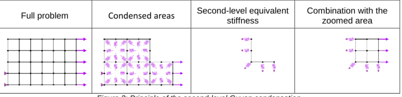
All subproblem associated to the condensed areas are combined, using assembly stiffness matrices. For the sake of clarity, only one condensed area will be considered. A second level of static
condensation is then performed on the condensed problem. The masternodes of this second-level condensation are the masternodes of the first-level condensation on the interface with the zoomed areas (Figure 1).
Full problem Condensed areas Second-level equivalent stiffness Combination with the zoomed area
Figure 3: Principle of the second-level Guyan condensation
The domain formed by the masternodes (𝑚) can be partitioned again in two subdomains 𝑀 and 𝐸, corresponding to the second-level masternodes and the eliminated masternodes:
7 1 , , , , 1 , , , , , ,
E m m s s s s M E m M E E E M m m m s s s s m M E M M
F
F
K
K F
F
U
U
U
K
K
K
K
K K
K
K
(6) with 𝐹E, 𝑈𝐸∈ ℝ𝑟, 𝐹𝑀, 𝑈𝑀∈ ℝ𝑠, 𝐾𝐸,𝐸 ∈ ℝ𝑟,𝑟, K𝐸,𝑀∈ ℝ𝑟,𝑠, 𝐾𝑀,𝐸∈ ℝ𝑠,𝑟, 𝐾𝐸,𝐸 ∈ ℝ𝑠,𝑠 , 𝑞 = 𝑟 + 𝑠. The system is condensed again to eliminate the displacement variables 𝑈𝐸. A system condensed on the level masternodes is obtained. The system size is then reduced to 𝑠 (number of second-level masternodes), compared to the 𝑞-dimensional system (4):1 1
, , , , , ,
(KM M KM EKE E KE M)UM FM KM EKE E FE (7)
This system is still equivalent to eq. (1) and (4). Its stiffness matrix is called the second-level
equivalent stiffness. It can then be combined with the problem modelling the zoomed areas (Figure 1), using assembly matrices. The combination of those problems forms the full condensed problem. 2.2.2 Adaptive zooming
2.2.2.1 Principle
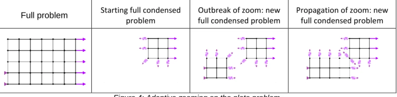
The principle of this zooming method raises the question of the propagation of zoomed zones but also of the apparition of new zones. Zooming on new areas includes changes in the model (mesh, behavior, properties, etc.) but also in the definition of the mechanical state of these new zoomed zones. In particular, this implies to modify the formulation of the problem when a new nonlinear behavior is detected. In our approach, when an adapted criterion is fulfilled, identified condensed areas are replaced by explicitly modelled areas. A change in the zoomed zones also implies a change in the applied equivalent stiffness, as the second-level masternodes change: The second-level condensation must be recalculated. However, the equivalent stiffness of each condensed area is never recalculated.
Full problem Starting full condensed problem
Outbreak of zoom: new full condensed problem
Propagation of zoom: new full condensed problem
Figure 4: Adaptive zooming on the plate problem
Figure 4 describes the simulation of the 2D plate problem with the adaptive zooming method, starting with only one zoomed area, and expanding the zoom to other areas when nonlinearities appear or propagate.
8
In order to obtain a condensed problem that is both correct and light to solve, new areas must be detected and zoomed as soon as nonlinearities occur in their behavior. Therefore a set of criteria (and the associated zooming thresholds) has to be defined to identify the linear and nonlinear areas. The zooming criteria are defined as follows and detailed in section 2.3:
The outbreak criterion detects the end of the linear phase of the behavior in an area: for instance multiple cracks in a structure under loading. This criterion applies to the condensed areas (and requires computing those areas).
The propagation criterion detects the nonlinearity propagation from a nearby area: for instance crack propagation in a fragile material or damage propagation alongside rebars in reinforced concrete. This criterion applies to the already zoomed areas (and requires no additional operations).
The zooming criteria depend on the nonlinear model chosen. The only common assumption is the presence of an elastic phase in the material models. It is to be noted that the zooming operation is currently irreversible: an area that has been zoomed is not condensed again (irreversible phenomena appear at the material level, such as permanent strain or changes in its mechanical properties).
2.2.2.2 Just-in-time zooming method
The zooming method is adapted to nonlinear problems approximated by numerical methods (such as FEM), discretized in time and solved incrementally, using an iterative method (such as the Newton-Raphson algorithm) at each loading increment [28]. The complete nonlinear problem is then considered as a large set of time steps problems solved sequentially. The full condensed problem is solved at each step, providing the solution of the nonlinear part of the full problem.
At the end of each loading step, the propagation zooming criterion is checked for all condensed areas and those areas can be zoomed if the criterion is met.
Since it is computationally more expensive (especially in damage mechanics simulations using nonlocal models), the outbreak criterion is usually checked less regularly. To guarantee that the condensation is valid, the condensed areas must stay in their linear phase between two criterion checks.
A first approach could consist in zooming slightly before the end of the linear phase (by lowering the zooming threshold on the outbreak criterion), to prevent nonlinearities from appearing between two checks. However, this method would need more empirically chosen parameters for the outbreak threshold and might be too conservative: because of the margin taken, areas may be zoomed although it would not be absolutely necessary.
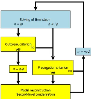
The “just-in-time zooming method” introduces a principle of retroactivity in the zooming method, by checking the zooming criteria after solving the full condensed problem on a step. Figure 5 describes the solving of a time step with the just-in-time zooming method. The criteria then behave differently:
The propagation criterion (immediate checking) directly causes zooming on the concerned areas.
9
The outbreak criterion (postponed checking) causes a return to the last verified step if needed, and zooming on the concerned areas.
Figure 5: Principle of a nonlinear simulation step with the just-in-time zooming method
This method runs on a hypothesis: it is assumed that a nonlinearity outbreak between steps (𝑛 + 1) and (𝑛 + 𝑝) will cause the outbreak criterion to match his threshold at step (𝑛 + 𝑝). This particularly implies that outbreak criterion checks must remain regular (𝑝 low). Choosing the value of this
checking frequency 𝑝 then becomes a compromise between the cost of solving several time steps twice and the cost of solving the condensed subproblems. If the major part of the structure is condensed, strongly nonlinear simulations might be faster with lower values of 𝑝 (even 𝑝 = 1) because the cost of solving steps would be high, whereas “almost linear” simulations might be faster with higher values of 𝑝, as the steps would be solved at low cost. Also, if nonlinearities are likely to appear in several distinct areas, lower values of 𝑝 should be used to detect those nonlinearities quickly. On the contrary, if nonlinearities are unlikely to appear in different areas, higher values of 𝑝 would increase computational performance.
This approach has been chosen because it eliminates the need to take margins on the zooming thresholds and compromise between computational efficiency (small margins) and safety on the linearity hypotheses (high margins). The major drawback of this approach is due to its retroactive framework: increments that lead to the outbreak of nonlinearities in condensed areas need to be computed again. This can cause higher computational cost: the frequency of outbreak criterion check must therefore be wisely chosen. Based on the cases presented in this contribution and other tests of concrete and reinforced concrete structures, values of 𝑝 chosen between 1 (strongly nonlinear problems) and 10 (weakly nonlinear problems) provide a good compromise.
10
2.3 Zooming criteria & parameters for reinforced concrete structures
2.3.1 Outbreak criterion
The outbreak criterion is a direct application of the model definition on condensed areas. Solving the linear subproblems of those areas and obtaining displacements of their internal degrees of freedom allows applying the numerical model on it (Figure 6). For instance on concrete mechanics modelled with the Mazars model [30], the criterion would be the equivalent strain 𝜀𝑒𝑞 , with the yield limit 𝜀0.
2 2 2
1 2 3
eq
(8)where are the principal positive values of the strain. i
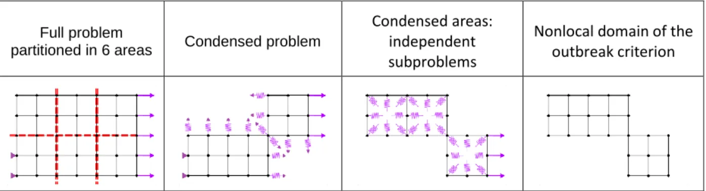
The outbreak zooming criterion is matched if the equivalent strain exceeds the elastic limit. If the simulation uses a nonlocal integral method (such as [31,32]), the zooming criterion shall be nonlocal (with the Mazars model, nonlocal equivalent strain). In this case, all the condensed subproblems are solved independently, giving the displacement and strain values, and eventually applying the model to compute additional variables, such as the equivalent strain. A nonlocal domain is then built, by reducing the global nonlocal domain (and connectivity matrices) of the full problem to its condensed part (which contains all condensed areas). Therefore, the nonlocal domain is not fractioned along the interface between two condensed areas (Figure 6): this avoids creating nonphysical strain localization on the interfaces (and therefore over-estimating the outbreak criterion [33,34]). The regularized variable (such as nonlocal equivalent strain) can then be calculated using the previously obtained values of the strain, and applying the regularization function on the nonlocal domain.
The purpose of this computation is solely to determine whether the elastic criterion is fulfilled. Thus, a linear computation is performed for the deformations. If the elastic criterion based on the nonlocal equivalent strain is met, the solution is acceptable, if not the zone is zoomed in.
The linear solving and model integration can easily be parallelized to speed up the simulation. However, solving the subproblems, applying the model and the nonlocal treatment can become computationally time-consuming operations on large problems, and that criterion must therefore be used parsimoniously.
Full problem
partitioned in 6 areas Condensed problem
Condensed areas: independent subproblems
Nonlocal domain of the outbreak criterion
Figure 6: Calculation of the outbreak criterion
2.3.2 Propagation criterion
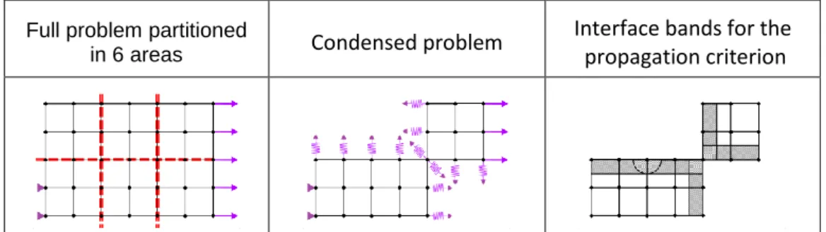
The propagation criterion is applied directly on the already zoomed areas. “Interface bands” are considered in the zoomed areas around each interface with a condensed area. The propagation criterion is measured on those bands and allows zooming on the condensed areas whose interface
11
bands match the criterion (Figure 7). The interface bands are defined by a thickness 𝐿, and include all nodes whose distance to a zoomed-condensed interface is smaller than 𝐿. If a nonlocal method is used with an internal length 𝑙𝐶0, the value of 𝐿 can be chosen depending on 𝑙𝐶0. This avoids
disequilibrium in the regularization domain near damaged areas, as nonlocal methods are known to be less accurate around the borders of the nonlocal domain. If no regularization technique is used, a value can be chosen depending on the mesh size. The propagation criterion applied in those
interface bands then depends on the model. In the case of concrete modelled with the Mazars model, a good choice is the damage variable D, with a null threshold. As this criterion is applied on already zoomed areas, and therefore on already computed variables, it has almost no computational cost, and can be applied very regularly.
Full problem partitioned
in 6 areas Condensed problem
Interface bands for the propagation criterion
Figure 7: Calculation of the propagation criterion
3 Application cases
The following examples illustrate the principle of the method and its usage on typical concrete and reinforced concrete structures. They show that the results of a full simulation are reproduced. The processor time (reflecting global computing load) is compared between simulations using the zooming method and reference simulations. The obtained speed-ups do not represent the point of the method, which is to allow access to finer simulations of large problems with limited computation resources. However, they provide a proof of concept for the structural zooming method, which has still to be optimized in order to obtain the best performance.
3.1 Three-point bending concrete beam
3.1.1 Problem description
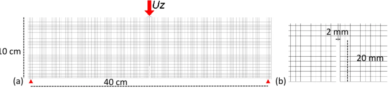
Figure 8 presents the finite element mesh of a notched plain concrete beam undergoing three-point bending, on which both reference simulations and experimental results are available. Both the experimental results, simulation hypotheses and model parameters are obtained from previous work published in work by Dufour et al. [35]. All simulations are run with Cast3M [28].
The beam is 40 cm long and 10 cm high (Figure 8). It is modelled in two dimensions under the hypothesis of plane stresses (the experimental beam is 5 cm wide). A notch is included at mid-span along the bottom of the beam, it is 2 mm large and 20 mm high (Figure 8). A regular quadrilateral mesh of size 2.5 mm is used with bilinear finite elements (6464 elements).
12
(a) (b)
Figure 8 : a: Mesh of the 2D notched beam (40x10 cm), with boundary and loading conditions. b: Mesh of the notch area (20x2 mm)
The material is modelled with the Mazars isotropic damage model[29], using the same parameters as in[34]. Those parameters give a compressive strength at 28 days 𝑓𝑐 equal to 41.4 MPa and a tensile strength 𝑓𝑡 equal to 3.03 MPa. To avoid mesh dependency, a nonlocal method is used: The stress-based regularization method [32], with the internal length lC0 = 7.5 mm has been chosen to limit the
spreading of nonlocal damage and get the right damage location initiation at the notch tip. The stress-based weighting function writes:
2
2
(
)
exp(
)
( , ( ))
cx
s
x
s
l
x
s
(9)The loading is applied at a point of a small area on the top of the beam (Figure 9). This small triangle-shaped area (2.5 mm x 12 mm) avoids the stress concentration around the loading point. At each support point, a similar rectangular-shaped elastic area (2.5 mm x 10 mm) is added to avoid geometrical singularities (Figure 9). Vertical displacement is blocked at each support point. The loading is an increasing vertical displacement up to 2x10⁻⁴ m. Horizontal displacement is free (except at the loading point).
(a) (b)
Figure 9 : a: Elastic loading area (yellow) b: Elastic boundary-conditions area (yellow)
3.1.2 Zooming method & criteria
The just-in-time structural zooming method is applied to this test case: The mesh of the beam is divided in 16 areas of equivalent dimension (Figure 10). An additional substructure is constituted with the elastic loading area. It is modelled from the start of the simulation, to support the displacement-driven loading. Although displacement-driven loadings are applied on the Lagrange multipliers, and could theoretically be condensed as displacement boundary conditions [29], it appears to be much simpler in terms of implementation (and has negligible computational cost) to model the loading area. On the contrary, the support areas are considered zoomable or condensable areas and associated to the adjacent zoomable zone. Boundary conditions are included in the equivalent structural stiffness.
2,5 mm 2,5 mm 20 mm 2 mm 10 cm 40 cm
13
Figure 10: Decomposition of the beam mesh in 17 areas
For the propagation criterion, a new adjacent zone is zoomed when damage is non-null in any element included (totally or partially) in a band 1.5 lC0 thick from the boundary (numerical damage
tolerance of 0.01, to avoid over-zooming when areas are small). For the outbreak criterion, if the nonlocal Mazars equivalent strain reaches 𝜀0 in a condensed zone, it will be zoomed. The outbreak criterion, which implies a costly computation on the condensed areas, is checked every four loading increments (𝑝 = 4), while the damage propagation criterion evaluation, which has negligible computing cost, is done at the end of every increment.
3.1.3 Comparison of the global behavior
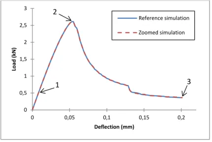
Figure 11 presents the load-deflection evolutions obtained with the zooming method and with the reference simulation (run with the same data but without zooming method). The deflection corresponds to the displacement of the central point of the beam.
Figure 11 : Load – Deflection evolution of the notched beam
Both curves follow the same evolution:
At point 1, damage initiates at the center of the beam. At point 2, the load peak is reached.
Point 3 is the last loading increment (and end of the simulations).
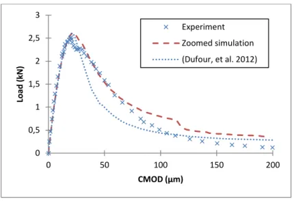
Figure 12 presents the Load-CMOD evolutions of our simulations (with the zoomed method), the experimental measures, and the simulation made in [35] with the same model and parameters (Figure 12). The CMOD is numerically calculated as the relative lateral displacement of the two points at the mouth of the notch.
0 0,5 1 1,5 2 2,5 3 0 0,05 0,1 0,15 0,2 Load (kN ) Deflection (mm) Reference simulation Zoomed simulation 1 3 2
14
Figure 12 : Load-CMOD evolution
The load-CMOD evolution shows that our simulation reproduces the experimental results quite correctly. Our simulation gives results closer to the experiment than [35]: this effect is due to the use of the stress-based regularization method, which allows better modelling of the behavior around the notch than the Gaussian regularization method.
3.1.4 Comparison of the local behavior
Figure 13 presents the damage profile evolutions for the reference simulation and the simulation using just-in-time zooming. For a given time step, both damage profiles are identical, with in both cases and evolution of the damage from the crack to the top of the beam. Some nonlinearities also appear near the supports. The structural zooming method models correctly the reference behavior of both condensed and zoomed area, including at the local scale.
Point 1 Point 2 Point 3
Figure 13 : Damage profiles at points 1 (appearance of damage), 2 (load peak), and 3 (end) for the reference simulation and the simulation with just-in-time zooming
3.1.5 Numerical efficiency
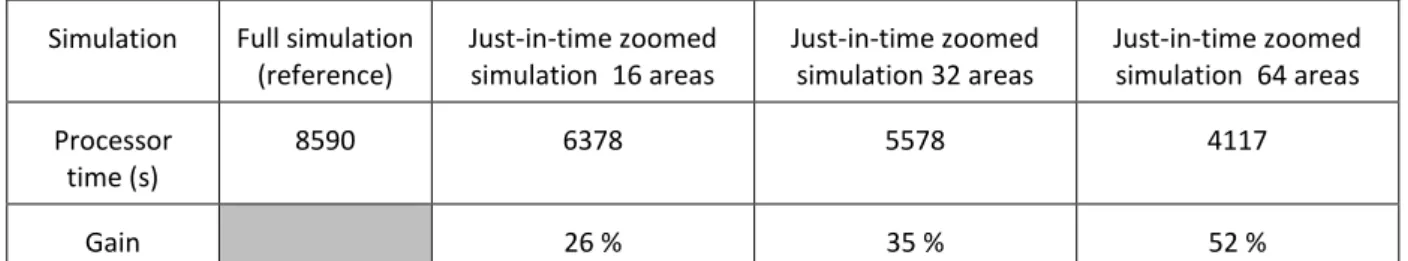
The computation times are also compared between the full simulation and the zoomed simulation. To observe the effect of the decomposition of the problem in zones, another zoomed simulation using the same dataset has been run, this time with the problem decomposed in 64 zoomable areas. All have been run on the same computer (a standard dual-core workstation) with Cast3M. Table 1 presents the processor times for all three simulations.
0 0,5 1 1,5 2 2,5 3 0 50 100 150 200 Lo ad ( kN ) CMOD (µm) Experiment Zoomed simulation (Dufour, et al. 2012)
15
Simulation Full simulation (reference) Just-in-time zoomed simulation 16 areas Just-in-time zoomed simulation 32 areas Just-in-time zoomed simulation 64 areas Processor time (s) 8590 6378 5578 4117 Gain 26 % 35 % 52 %
Table 1 : Processor times for the simulation of the notched concrete beam (actual duration of the simulations are smaller than those since the processor used is dual-core)
These processor times show an economy of respectively 26%, 35% and 52% when using the just-in-time zooming method with 16, 32 and 64 zoomable areas (Table 1). The better results obtained with the 64 areas configuration can be explained by the shape and localization of the damage in the structure, leading the 64 areas simulation to run with a lower part of the beam modelled (Figure 14). This clearly demonstrates the interest of this area-condensation approach. Although the absolute speed-up values may seem low compared to other zooming or model reduction methods, it must be kept in mind that the results are identical to those of the full simulation.
Even with better optimization of the method and its parameters, what appears from the damage profiles (Figure 14) is that the shape of the zoomed area matches the damage distribution in the beam. With the finest decomposition (64 areas), the speed-up is therefore limited only by the distribution of damage in the structure. The ratio of zoomed to condensed areas is expected to be much higher on large structures since the damaged areas are supposed to be small. The economy in computational load, and thus the ability to access more refined simulation with given computational power, is expected to scale.
Point 1 Point 2 Point 3
Figure 14 : Damage profiles for the zoomed simulation with 16 areas and the zoomed simulation with 64 areas
3.2 Reinforced concrete structure under internal pressure
3.2.1 Problem description
This test case aims to evaluate the applicability of the method to a structure which represents a reinforced concrete containment building mock-up. The structure is a reinforced concrete cylinder with a hemispherical dome. The displacements at the bottom of the cylinder are blocked and the structure undergoes an internal pressure loading.
16
(a) (b) (c) (d)
Figure 15: Mesh of the simplified containment building a: Mesh of the concrete
b: Mesh of the steel rebars c: Zoomable areas of the structure
d: Distribution of the random Young’s modulus of concrete
Figure 15 presents the mesh and geometry of the reinforced concrete structure. Table 2 presents its dimensions.
Cylinder height Cylinder external radius
Cylinder thickness Dome external radius
Dome thickness
13.3 m 7.3 m 40 cm 7.3 m 40 cm
Table 2: Dimensions of the reinforced concrete
The concrete cylinder is meshed with rectangle parallelepipeds (50 cm x 50 cm x 40 cm, one element in the thickness), and the dome with prismatic elements, both with tri-linear finite elements. The steel rebars are modelled with truss finite elements (50 cm). Those truss elements have an equivalent section 𝑆 = 8.04 cm2 (corresponding to a steel diameter of 32 mm). All 12 horizontal circular rebars are inserted at 17.5 cm thickness (from inside) in the cylinder, 40 vertical rebars are inserted at 22.5 cm thickness in the cylinder, and 80 in the dome. The link between rebars and the concrete volume is ensured by kinematic relations on nodal displacement.
The concrete is modelled using the Mazars isotropic damage model, with the parameters given in Table 3. For a mean Young’s modulus of 𝐸𝑀= 30 GPa, this gives a compressive strength at 28 days 𝑓𝑐 of 26.9 MPa and a tensile strength 𝑓𝑡 of 3.0 MPa. A random auto-correlated field is used to
represent an heterogeneity in the concrete Young’s modulus at the structural scale. Although it is not technically required for this analysis, this random field modelling has two functions: firstly, it gives a closer representation of the physics of a nuclear pressure vessel’s, where mechanical properties are known to vary spatially [36]; secondly, using heterogeneous properties allows to break the problem’s rotational invariance, and creates weaker points where damage can localize. The distribution follows a Gaussian law with a mean value 𝐸𝑀 equal to 30 GPa and a standard deviation 𝐸𝜎 equal to 3.0 GPa (Figure 15). The chosen spatial autocorrelation function is arbitrarily Gaussian with an
autocorrelation length 𝑙𝑖 = 1 m. The steel rebars are modelled using the Von Mises plasticity model with linear hardening (see parameters given in Table 4).
17 Young’s modulus Poisson Coefficient Damage threshold A (compression) B (compression) A (tension) B (tension) Shear coefficient 𝐸𝑀 𝜈 𝜀0 𝐴𝑐 𝐵𝑐 𝐴𝑇 𝐵𝑇 𝛽 30 GPa 0.2 1x10⁻⁴ 1.15 1900 0.95 12000 1.06
Table 3: Parameters of the Mazars model for the cylinder’s concrete
Young’s modulus Yield strain Yield stress Maximum strain Maximum strength Section
𝐸 𝜀𝑦 𝜎𝑦 𝜀𝑚 𝜎𝑚 𝑆
200 GPa 2x10⁻³ 400 MPa 5x10⁻² 600 MPa 8.04 cm2
Table 4: Parameters of the plasticity model for the cylinder’s steel rebars
To avoid mesh dependency, a nonlocal method is used: The stress-based regularization method [32], with the internal length lC0 = 0.5 m has been chosen to limit the spreading of nonlocal damage.
The loading is a uniform pressure applied on the internal surface of the cylinder and the dome, up to 1.73x10⁵ Pa.
3.2.2 Zooming method & criteria
The structural zooming method is applied on this simulation: The mesh of the structure is divided in 6 zoomable areas of equivalent dimension (Figure 15). All boundary conditions applicable are
condensed in the equivalent stiffness. The applied loading is also condensed when necessary. The zooming criteria used on the concrete model are the same as the plain concrete beam case, since the same mechanical model is used. No zooming criterion is applied for the steel model since its degrees of freedom are kinematically linked to the concrete nodes, and its mechanical model will allow larger values of strain in the linear-elastic phase: Therefore, the steel will be zoomed or condensed following the concrete of the area.
3.2.3 Results
Figure 16 presents pressure-displacement evolutions for the reference and zoomed simulations. In both cases, the same field is considered for the concrete Young’s modulus.
Figure 16: Pressure-displacement evolution, and its nonlinear phase
0,00 0,10 0,20 0,30 0,40 0,50 0,60 0,70 0,80 0,00 0,50 1,00 1,50 2,00 R adi al di spl acem e nt (m m )
Internal pressure (bar) Reference Zoom 0,58 0,60 0,62 0,64 0,66 0,68 0,70 1,45 1,50 1,55 1,60 1,65 1,70 R adi al di spl acem e nt (m m )
Internal pressure (bar) Reference Zoom
18
Figure 16 shows a total agreement between both simulations. This confirms the results on the concrete beam, and the applicability of the method to a tridimensional problem with reinforcement bars (and therefore, multiple mechanical models).
Figure 17: Final damage distribution for the reference simulation and zoomed simulation
The damage profiles (Figure 17) at the last step also show a total agreement between the zoomed simulation and the reference simulation, on both localization and values of the damage variable. The results of the reference simulation are then correctly reproduced by the simulation using the
structural zooming method.
The computation times are compared. Both simulations have been run on the same computer (a 16-core computing node).
Simulation Full simulation (reference) Zoomed simulation / 6 areas Processor time (s) 1838 922
Table 5: Processor times for the simulation of the simplified reinforced concrete containment building
Those processor times show an economy induced by the use of the zooming method of 50% (Table 5). The zooming method’s applicability and usefulness is therefore confirmed on that type of simulations. The observation of the simulation’s evolution reveals that the outbreak criterion is matched only once. However, given the small number of steps effectively computed (27 steps), higher values of 𝑝 would most likely induce a lower performance, as a large part of the simulation would be computed twice. However, with finer meshes, new problem decompositions could be proposed to keep the computational cost low while refining the simulation.
4 Conclusions
An adaptive condensation method for the nonlinear simulation of large structures has been
presented. It uses Guyan degree of freedom elimination to reduce the dimension of a large problem with localized nonlinear behavior. When the system evolves during the loading, our method allows an evolution of the zoomed areas (propagation or outbreak). This method can be applied to any model and material with suitable zooming criteria. The more localized the nonlinearities are, the more efficient the method will be.
This method has been applied on two computational test cases. The first case is a plain concrete notched beam under a three-point bending. On this case the method can reproduce the results of a
19
reference simulation with accuracy and provides a speed-up greater than 2 in computation time with standard and non-optimized parameters. The performance is expected to be higher with optimal parameters (initial zone decomposition especially) and an optimized implementation. The second test case is a reinforced concrete structure model whose geometry corresponds to the simplified shape and dimensions of a nuclear confinement building mock-up. On this case, the zooming method can also reproduce the reference computation with accuracy. An economy of 50 % computation time is observed, thus confirming the efficiency of the method.
However, the computational efficiency of the method can only be measured for given test cases, since it is highly dependent on the subproblems decomposition, and most of all, on the localization of nonlinearities on a small area. The structural zooming method reduces the size of the problem solved to that of the sole nonlinear area (and not of the full problem): for a given size of nonlinear area, the efficiency of the method will increase with the size of the problem. Small- and intermediate-scale problems are therefore intrinsically unfavorable to the method. On strongly localized nonlinear problems, such as concrete cracking in large structures including several heterogeneities, a higher performance is expected, giving access to the solution of larger problems.
Ongoing research will focus on a method to condense again the damaged areas in which the stiffness does not evolve anymore due to damage saturation and parametric studies on both the problem decomposition and the criterion checking frequency in order to find some optimal values for the method parameters.
Acknowledgements
The authors gratefully acknowledge the funding support from France’s National Research Agency through “MACENA” project (ANR-11-RSNR-012).
References
[1] R.J. Guyan, Reduction of stiffness and mass matrices, AIAA Journal. 3 (1965) 380–380. doi:10.2514/3.2874.
[2] F. Feyel, J.-L. Chaboche, FE2 multiscale approach for modelling the elastoviscoplastic behaviour of long fibre SiC/Ti composite materials, Computer Methods in Applied Mechanics and
Engineering. 183 (2000) 309–330. doi:10.1016/S0045-7825(99)00224-8.
[3] P. Ladevèze, O. Loiseau, D. Dureisseix, A micro–macro and parallel computational strategy for highly heterogeneous structures, Int. J. Numer. Meth. Engng. 52 (2001) 121–138.
doi:10.1002/nme.274.
[4] P. Ladevèze, A. Nouy, On a multiscale computational strategy with time and space homogenization for structural mechanics, Computer Methods in Applied Mechanics and Engineering. 192 (2003) 3061–3087. doi:10.1016/S0045-7825(03)00341-4.
[5] H.B. Dhia, G. Rateau, The Arlequin method as a flexible engineering design tool, Int. J. Numer. Meth. Engng. 62 (2005) 1442–1462. doi:10.1002/nme.1229.
20
[6] T. Belytschko, S. Loehnert, J.-H. Song, Multiscale aggregating discontinuities: A method for circumventing loss of material stability, Int. J. Numer. Meth. Engng. 73 (2008) 869–894. doi:10.1002/nme.2156.
[7] G. Cusatis, L. Cedolin, Two-scale study of concrete fracturing behavior, Engineering Fracture Mechanics. 74 (2007) 3–17. doi:10.1016/j.engfracmech.2006.01.021.
[8] J. Rousseau, E. Frangin, P. Marin, L. Daudeville, Multidomain finite and discrete elements method for impact analysis of a concrete structure, Engineering Structures. 31 (2009) 2735– 2743. doi:10.1016/j.engstruct.2009.07.001.
[9] K. Haidar, J.F. Dubé, G. Pijaudier-Cabot, Modelling crack propagation in concrete structures with a two scale approach, Int. J. Numer. Anal. Meth. Geomech. 27 (2003) 1187–1205. doi:10.1002/nag.318.
[10] J. Mandel, Balancing domain decomposition, Communications in Numerical Methods in Engineering. 9 (1993) 233–241. doi:10.1002/cnm.1640090307.
[11] C. Dohrmann, A Preconditioner for Substructuring Based on Constrained Energy Minimization, SIAM J. Sci. Comput. 25 (2003) 246–258. doi:10.1137/S1064827502412887.
[12] C. Farhat, F.-X. Roux, A method of finite element tearing and interconnecting and its parallel solution algorithm, Int. J. Numer. Meth. Engng. 32 (1991) 1205–1227.
doi:10.1002/nme.1620320604.
[13] C. Farhat, J. Mandel, The two-level FETI method for static and dynamic plate problems Part I: An optimal iterative solver for biharmonic systems, Computer Methods in Applied Mechanics and Engineering. 155 (1998) 129–151. doi:10.1016/S0045-7825(97)00146-1.
[14] C. Farhat, M. Lesoinne, P. LeTallec, K. Pierson, D. Rixen, FETI-DP: a dual–primal unified FETI method—part I: A faster alternative to the two-level FETI method, Int. J. Numer. Meth. Engng. 50 (2001) 1523–1544. doi:10.1002/nme.76.
[15] R.W. Clough, E.L. Wilson, Dynamic analysis of large structural systems with local nonlinearities, Computer Methods in Applied Mechanics and Engineering. 17–18, Part 1 (1979) 107–129. doi:10.1016/0045-7825(79)90084-7.
[16] J. Lumley, The structure of inhomogeneous turbulent flows, 1967.
[17] P. Spanos, R. Ghanem, Stochastic Finite Element Expansion for Random Media, J. Eng. Mech. 115 (1989) 1035–1053. doi:10.1061/(ASCE)0733-9399(1989)115:5(1035).
[18] G. Berkooz, P. Holmes, J.L. Lumley, The Proper Orthogonal Decomposition in the Analysis of Turbulent Flows, Annu. Rev. Fluid Mech. 25 (1993) 539–575.
doi:10.1146/annurev.fl.25.010193.002543.
[19] C. Soize, Reduced models in the medium frequency range for general dissipative structural-dynamics systems, European Journal of Mechanics - A/Solids. 17 (1998) 657–685.
21
[20] A. Batou, C. Soize, N. Brie, Reduced-order computational model in nonlinear structural dynamics for structures having numerous local elastic modes in the low-frequency range. Application to fuel assemblies, Nuclear Engineering and Design. 262 (2013) 276–284. doi:10.1016/j.nucengdes.2013.04.039.
[21] H.M. Panayirci, H.J. Pradlwarter, G.I. Schuëller, Efficient stochastic structural analysis using Guyan reduction, Advances in Engineering Software. 42 (2011) 187–196.
doi:10.1016/j.advengsoft.2011.02.004.
[22] S.R. Idelsohn, A. Cardona, A reduction method for nonlinear structural dynamic analysis, Computer Methods in Applied Mechanics and Engineering. 49 (1985) 253–279.
doi:10.1016/0045-7825(85)90125-2.
[23] O.P. Agrawal, K.J. Danhof, R. Kumar, A superelement model based parallel algorithm for vehicle dynamics, Computers & Structures. 51 (1994) 411–423. doi:10.1016/0045-7949(94)90326-3. [24] I. Hirai, B.P. Wang, W.D. Pilkey, An efficient zooming method for finite element analysis, Int. J.
Numer. Meth. Engng. 20 (1984) 1671–1683. doi:10.1002/nme.1620200910.
[25] I. Hirai, Y. Uchiyama, Y. Mizuta, W.D. Pilkey, An exact zooming method, Finite Elements in Analysis and Design. 1 (1985) 61–69. doi:10.1016/0168-874X(85)90008-3.
[26] B.P. Wang, W.D. Pilkey, Efficient reanalysis of locally modified structures, in: First Chautauqua on Finite Element Modeling, Wallace Press, Harwichport, MA, 1980: pp. 37–62.
[27] A.K. Noor, Global-local methodologies and their application to nonlinear analysis, Finite Elements in Analysis and Design. 2 (1986) 333–346. doi:10.1016/0168-874X(86)90020-X. [28] CEA, Description of the finite element code Cast3M, (2014). http://www-cast3m.cea.fr/. [29] J. Pellet, Dualisation of the boundary conditions, in: Code_Aster Open Source - General FEA
Software, 2011. http://www.code-aster.org/V2/doc/default/en/man_r/r3/r3.03.01.pdf. [30] J. Mazars, G. Pijaudier-Cabot, Continuum Damage Theory - Application to Concrete, J. Eng.
Mech. 115 (1989) 345–365. doi:10.1061/(ASCE)0733-9399(1989)115:2(345).
[31] G. Pijaudier-Cabot, Z.P. Bažant, Nonlocal Damage Theory, J. Eng. Mech. 113 (1987) 1512–1533. doi:10.1061/(ASCE)0733-9399(1987)113:10(1512).
[32] C. Giry, F. Dufour, J. Mazars, Stress-based nonlocal damage model, International Journal of Solids and Structures. 48 (2011) 3431–3443. doi:10.1016/j.ijsolstr.2011.08.012.
[33] A. Krayani, G. Pijaudier-Cabot, F. Dufour, Boundary effect on weight function in nonlocal damage model, Engineering Fracture Mechanics. 76 (2009) 2217–2231.
doi:10.1016/j.engfracmech.2009.07.007.
[34] G. Pijaudier-Cabot, F. Dufour, Non local damage model, European Journal of Environmental and Civil Engineering. 14 (2010) 729–749. doi:10.1080/19648189.2010.9693260.
22
[35] F. Dufour, G. Legrain, G. Pijaudier-Cabot, A. Huerta, Estimation of crack opening from a two-dimensional continuum-based finite element computation, Int. J. Numer. Anal. Meth. Geomech. 36 (2012) 1813–1830. doi:10.1002/nag.1097.
[36] T. de Larrard, J.B. Colliat, F. Benboudjema, J.M. Torrenti, G. Nahas, Effect of the Young modulus variability on the mechanical behaviour of a nuclear containment vessel, Nuclear Engineering and Design. 240 (2010) 4051–4060. doi:10.1016/j.nucengdes.2010.09.031.