HAL Id: hal-02566420
https://hal.archives-ouvertes.fr/hal-02566420
Submitted on 21 Jul 2020
HAL is a multi-disciplinary open access
archive for the deposit and dissemination of
sci-entific research documents, whether they are
pub-lished or not. The documents may come from
teaching and research institutions in France or
abroad, or from public or private research centers.
L’archive ouverte pluridisciplinaire HAL, est
destinée au dépôt et à la diffusion de documents
scientifiques de niveau recherche, publiés ou non,
émanant des établissements d’enseignement et de
recherche français ou étrangers, des laboratoires
publics ou privés.
analysis of the edge-on Be star o Aquarii
E. S. G. de Almeida, A. Meilland, A. Domiciano de Souza, P. Stee, D.
Mourard, N. Nardetto, R. Ligi, I. Tallon-Bosc, D. Faes, A. Carciofi, et al.
To cite this version:
E. S. G. de Almeida, A. Meilland, A. Domiciano de Souza, P. Stee, D. Mourard, et al.. Visible and
near-infrared spectro-interferometric analysis of the edge-on Be star o Aquarii. Astronomy and Astrophysics
- A&A, EDP Sciences, 2020, 636, pp.A110. �10.1051/0004-6361/201936039�. �hal-02566420�
Astronomy
&
Astrophysics
https://doi.org/10.1051/0004-6361/201936039© E. S. G. de Almeida et al. 2020
Visible and near-infrared spectro-interferometric analysis of the
edge-on Be star o Aquarii
E. S. G. de Almeida
1, A. Meilland
1, A. Domiciano de Souza
1, P. Stee
1, D. Mourard
1, N. Nardetto
1, R. Ligi
2,
I. Tallon-Bosc
3, D. M. Faes
4, A. C. Carciofi
4, D. Bednarski
4, B. C. Mota
4, N. Turner
5, and T. A. ten Brummelaar
51Université Côte d’Azur, Observatoire de la Côte d’Azur, CNRS, Laboratoire Lagrange, France
e-mail: [email protected]
2 INAF – Osservatorio Astronomico di Brera, Via E. Bianchi 46, 23807 Merate, Italy
3Univ. Lyon, Univ. Lyon1, ENS de Lyon, CNRS, Centre de Recherche Astrophysique de Lyon UMR5574, 69230 Saint-Genis-Laval,
France
4Instituto de Astronomia, Geofísica e Ciências Atmosféricas, Universidade de São Paulo, São Paulo, Brazil
5CHARA Array - Georgia State University, Mount Wilson, CA, USA
Received 6 June 2019 / Accepted 6 February 2020
ABSTRACT
Aims. We present a detailed visible and near-infrared spectro-interferometric analysis of the Be-shell star o Aquarii from
quasi-contemporaneous CHARA/VEGA and VLTI/AMBER observations.
Methods. We analyzed spectro-interferometric data in the Hα (VEGA) and Brγ (AMBER) lines using models of increasing
complex-ity: simple geometric models, kinematic models, and radiative transfer models computed with the 3D non-LTE code HDUST.
Results. We measured the stellar radius of o Aquarii in the visible with a precision of 8%: 4.0 ± 0.3 R . We constrained the
circum-stellar disk geometry and kinematics using a kinematic model and a MCMC fitting procedure. The emitting disk sizes in the Hα and Brγ lines were found to be similar, at ∼10–12 stellar diameters, which is uncommon since most results for Be stars indicate a larger
extension in Hα than in Brγ. We found that the inclination angle i derived from Hα is significantly lower (∼15◦) than the one derived
from Brγ: i ∼ 61.2◦and 75.9◦, respectively. While the two lines originate from a similar region of the disk, the disk kinematics were
found to be near to the Keplerian rotation (i.e., β = −0.5) in Brγ (β ∼ −0.43), but not in Hα (β ∼ −0.30). After analyzing all our data using a grid of HDUST models (BeAtlas), we found a common physical description for the circumstellar disk in both lines: a base disk
surface density Σ0= 0.12 g cm−2and a radial density law exponent m = 3.0. The same kind of discrepancy, as with the kinematic model,
is found in the determination of i using the BeAtlas grid. The stellar rotational rate was found to be very close (∼96%) to the critical value. Despite being derived purely from the fit to interferometric data, our best-fit HDUST model provides a very reasonable match to non-interferometric observables of o Aquarii: the observed spectral energy distribution, Hα and Brγ line profiles, and polarimetric quantities. Finally, our analysis of multi-epoch Hα profiles and imaging polarimetry indicates that the disk structure has been (globally) stable for at least 20 yr.
Conclusions. Looking at the visible continuum and Brγ emission line only, o Aquarii fits in the global scheme of Be stars and their
circumstellar disk: a (nearly) Keplerian rotating disk well described by the viscous decretion disk (VDD) model. However, the data in the Hα line shows a substantially different picture that cannot fully be understood using the current generation of physical models of Be star disks. The Be star o Aquarii presents a stable disk (close to the steady-state), but, as in previous analyses, the measured m is lower than the standard value in the VDD model for the steady-state regime (m = 3.5). This suggests that some assumptions of this model should be reconsidered. Also, such long-term disk stability could be understood in terms of the high rotational rate that we measured for this star, the rate being a main source for the mass injection in the disk. Our results on the stellar rotation and disk stability are consistent with results in the literature showing that late-type Be stars are more likely to be fast rotators and have stable disks. Key words. stars: individual: o Aquarii – stars: emission-line, Be – circumstellar matter – techniques: interferometric
1. Introduction
Classical Be stars are main-sequence B-type stars that show (or showed at some time) Balmer lines in emission and infrared excess in their spectral energy distribution. The Be phenomenon is found among the entire spectral range of B stars (e.g.,
Townsend et al. 2004): M?from ∼3 M (B9, Teff∼ 12 000 K), up to ∼18 M (B0, Teff∼ 30 000 K). These observational character-istics are well explained as arising from a dust-free gaseous disk that is supported by rotation with a slow radial velocity (see, e.g.,
Rivinius et al. 2013). The most successful theory to explain the evolution of the disk structure is the so-called viscous decretion disk (VDD) model, where its dynamics are driven by viscosity (e.g.,Lee et al. 1991;Okazaki 2001;Bjorkman & Carciofi 2005).
It is widely accepted that fast rotation plays an important role in the formation of the Be star disk. However, while interferomet-ric analyses typically provide rotational rates vrot/vcrit& 0.7 (e.g.,
Meilland et al. 2012;Cochetti et al. 2019), some statistical stud-ies show rates ranging from ∼0.3 up to 1.0 (e.g.,Cranmer 2005;
Zorec et al. 2016). Moreover, it is still not clear whether the rota-tional rate is correlated to other stellar parameters such as the effective temperature (e.g.,Cochetti et al. 2019). Hence, despite the success of the VDD model, the physical mechanism(s) driv-ing the mass injection remains unclear and a detailed physical characterization for the central star and the disk structure is mandatory to better understand the Be phenomenon. By gaining access to geometry on the milliarcsecond scale and kinematics on a few tens of km s−1 scale, spectro-interferometry offers a
A110, page 1 of23
unique opportunity to probe the circumstellar environment and stellar surfaces of Be stars (see, e.g.,Chesneau et al. 2012;Stee & Meilland 2012).
The bright, late-type Be star (type B7IVe) o Aquarii (HD 209409) is known to have a fairly stable disk (Sigut et al. 2015). The stability of the circumstellar disk is evidenced by the quasi-constant equivalent width in the Hα line, double-peak sep-aration, and the absence of long-term violet-to-red (V/R) peak variations (e.g., Rivinius et al. 2006; Sigut et al. 2015). This star shows a high value of v sin i ∼ 282 km s−1 (Frémat et al.
2005) and a shell absorption in Hα, thus indicating a high stellar inclination angle of about 70◦, as discussed below.
Meilland et al. (2012) presented the first
spectro-interferometric analysis of o Aquarii with the VLTI/AMBER instrument as part of their AMBER survey of eight bright Be stars. Despite the low data quality and very limited number of observations (just one measurement), they were able to signifi-cantly constrain the disk geometry and kinematics. They found that the disk emission in the Brγ line, modeled as an elliptical Gaussian distribution, had a FWHM of 14 ± 1 D? (with R?= 4.4 R ), where D?and R?are, respectively, the stellar diameter and radius. They estimated the inclination angle as i = 70 ± 20◦ and found a stellar rotational rate of vrot/vcrit= 0.77 ± 0.21 (Ω/Ωc= 0.93+0.06−0.17), where vcrit and Ωcrit are, respectively, the linear and angular critical velocity. New VLTI/AMBER spectro-interferometric measurements of o Aquarii were presented in the Be star survey ofCochetti et al.(2019). Here, they obtained seven good-quality measurements for o Aquarii (i.e., 21 base-lines). Using a similar model as inMeilland et al.(2012), they found a Brγ emission FWHM significantly smaller than in
Meilland et al.(2012), 8 ± 0.5 D?(with R?= 4.4 R ), and better constrained the object inclination angle (70 ± 5◦).
A detailed analysis of o Aquarii using Hα spectroscopy and interferometry was performed bySigut et al.(2015). These authors combined large band (15 nm) interferometric data cen-tered on Hα, obtained from the Navy Precision Optical Interfer-ometer (NPOI), with Hα spectroscopy from the Lowell Obser-vatory Solar-Stellar Spectrograph. Using the radiative transfer code BEDISK (Sigut & Jones 2007), they were able to reproduce simultaneously the visibility, Hα line profile, and spectral energy distribution (SED), and showed that the disk is quite stable for up to about ten years. Interestingly, they found a disk extension in Hα (Gaussian FWHM of 12.0 ± 0.5 D?) close to the one deter-mined byMeilland et al.(2012) in Brγ (FWHM of 14 ± 1 D?). They concluded that this is uncommon since most previously studied Be stars exhibit a larger (up to two times) disk emission region in Hα than in Brγ.
In this paper, we present new CHARA/VEGA spectro-interferometric measurements of o Aquarii centered on the Hα emission line (λ = 0.656 µm). They are analyzed conjointly with the AMBER Brγ line (λ = 2.166 µm) measurements from
Meilland et al.(2012) andCochetti et al.(2019), using models of increasing complexity: simple geometric models, kinematic models, and radiative transfer models. This is the first time the code HDUST has been used to model simultaneously spectro-interferometric data from Hα and Brγ. It is the second time for the kinematic model (i.e., after the δ Scorpii data published inMeilland et al. 2011). This multi-wavelength and multi-line approach allows us to draw a more complete picture of the stellar surface and circumstellar environment of the Be star o Aquarii.
This paper is organized as follows. In Sect.2, we present the observations and the data reduction process. Our analysis using geometric models of the VEGA calibrated (absolute) visibility is shown in Sect.3. In Sect.4, we fit the VEGA and AMBER
differential visibility and phase with a kinematic model using a Markov chain Monte Carlo (MCMC) model fitting method. In Sect.5, all the interferometric data are analyzed in terms of 3D non-LTE radiative transfer models. Our kinematic and radiative transfer models are discussed in Sect.6. In Sect.7, our best-fit models are compared to non-interferometric observables: the spectral energy distribution and line profiles (Hα and Brγ). The comparison with polarimetric data is performed in Sect.8.4.3in the context of the disk stability. In Sect.8, we discuss the mor-phological, kinematic, and physical descriptions for o Aquarii and its circumstellar disk. Our conclusions are summarized in Sect.9.
2. Observations
2.1. CHARA/VEGA
The VEGA instrument (Mourard et al. 2009) is one of the two visible beam combiners on the CHARA Array (ten Brummelaar et al. 2005). It can simultaneously combine up to four beams, operating at different wavelengths from 450 to 850 nm. VEGA is equipped with two cameras (blue and red detectors) that can observe in two different spectral domains simultaneously (around the Hβ and the Hα lines). Currently, it is the only instrument at the CHARA Array with a spectral resolution high enough to resolve narrow spectral features such as atomic and molecular lines. It offers 3 spectral modes: R = 1000 (LR), R = 6000 (MR), and R = 30 000 (HR).
o Aquarii was observed 50 times with VEGA between 2012 and 2016 in MR mode centered on the Hα emission line at 0.656 µm. The 2012 and 2016 observations were focused on the disk geometry and kinematics and data were taken with small baselines (up to 105 m) and without stellar calibrators. On the other hand, the 2013 and 2014 campaigns were aimed at constraining not only the Hα emission, but also the R-band con-tinuum geometry. Consequently, observations were carried out with longer baselines (up to 330 m) with a standard calibration plan alternating observations of the science target and few cal-ibrator stars chosen using the SearchCal (Bonneau et al. 2006) tool developed by the Jean-Marie Mariotti Center (JMMC)1.
TableA.1shows useful information about the stars used as inter-ferometric calibrators during these campaigns. The complete log of observations is presented in Table A.2and the correspond-ing uv plane coverage for the VEGA observations is plotted in Fig.1.
Data were reduced using the standard VEGA data reduction software2 described inMourard et al.(2012). For all programs,
differential visibility and phases were computed from the inter-correlation between a fixed 15 nm window centered on Hα and a sliding smaller window (i.e. 1, 2, or 5 Å, depending on the data quality). For the 2013 and 2014 data, the raw squared visibility was computed for o Aquarii, and its calibrators, using the auto-correlation method on a 15 nm band centered on the Hα emission line (649–664 nm) and another band in the close-by contin-uum (635–650 nm). Then the transfer function was estimated assuming the diameter of the calibrators recorded before and after the science target observation, and its uncertainty using a weighted standard deviation. Finally, for each measurement, the calibrated squared visibility was derived by dividing o Aquarii’s raw squared visibility by the estimated transfer function. 1
https://www.jmmc.fr/english/tools/proposal-preparation/search-cal/
300
200
100
0
100
200
300
u (m)
300
200
100
0
100
200
300
v (m)
Fig. 1. uv plan coverage obtained around Hα (0.656 µm) with CHARA/VEGA (green) and Brγ (2.166 µm) with VLTI/AMBER (red).
2.2. VLTI/AMBER
The AMBER instrument (Petrov et al. 2007) was a three-beam combiner (decommissioned in 2018) at the Very Large Tele-scope Interferometer (VLTI). It operated in the H- and K-bands with three spectral resolutions: R = 35 (LR), R = 1500 (MR), and R = 12 000 (HR). It offered the highest spectral resolution at the VLTI, being the most adapted for studying the gaseous environment in emission lines.
o Aquarii was observed with AMBER during two observ-ing surveys of Be stars in 2011 (ESO program 087.D-0311) and in 2014 (ESO program 094.D-0140). The observations were per-formed in HR mode in K-band centered on the Brγ emission line at 2.166 µm. The data from 2011 was published inMeilland et al.
(2012) and the 2014 data inCochetti et al.(2019). During this second survey, seven measurements were acquired for o Aquarii with three different triplets. The log of AMBER observations is also presented in TableA.2and the corresponding uv plane coverage is plotted in Fig.1.
Calibration was performed using similar methods as the one described for VEGA. However, AMBER measurements were often affected by a highly variable transfer function mainly due to the variable quality of the fringe tracking performed by the FINITO fringe tracker, during the long exposure time needed to perform HR mode observations. As it was the case during our o Aquarii observations, we present in this paper only the anal-ysis of differential measurements obtained using the standard AMBER data reduction software amdlib (Tatulli et al. 2007;
Chelli et al. 2009).
3. Geometric modeling: VEGA calibrated visibility
In this section, we fit the Hα and continuum squared visibili-ties (V2) from the VEGA observations where calibrators were observed. We note that as the AMBER data were not calibrated, such analysis cannot be performed on the K-band continuum and Brγ line.
To determine if we can separate the circumstellar disk and the stellar photosphere emissions and constrain their geome-try independently, we fitted our data with geometric models of increasing complexity: one-component models (uniform disk, UD, or a uniform ellipse) and two-component models (UD plus UD, Gaussian disk, or uniform or Gaussian ellipse).
0 100 200 300 400 500 0.0 0.2 0.4 0.6 0.8 1.0 1.2 V 2 continuum (635-650nm) 0 100 200 300 400 500 B (m) 0.0 0.2 0.4 0.6 0.8 1.0 1.2 V 2 H (649-664nm)
Fig. 2.VEGA V2measurements in the close-by continuum band (top)
and in the Hα band (bottom) are shown in red points. Our best-fit models consisting of one (solid line) and two (dashed line) uniform disks are
overplotted in blue. See Table1and text for discussion.
Here, the first component represents the stellar surface and the second one the circumstellar disk. To perform our fit, we used the LITpro model fitting software (Tallon-Bosc et al. 2008) for optical and infrared interferometric observations developed by the Jean-Marie Mariotti Center (JMMC)3.
In Fig. 2, we show the comparison between the visibility curves of our best-fit models to the VEGA data both in the continuum and Hα bands. One sees that the object is partially resolved in the continuum and the Hα line. The lower level of the visibility in the band centered on the Hα line clearly shows that the object is larger in Hα than in the close-by continuum region. Assuming that the emission originates from both the stellar pho-tosphere and a circumstellar disk, the lower visibility in Hα is due to a larger fraction of the Hα flux coming from the disk than from the star. In contrast, the flux contribution from the star is greater than that from the disk in the continuum R-band.
Our main results are summarized in Table1. We only show our results using UD models since there is no improvement in terms of reduced χ2(χ2
r) when considering more complex mod-els, that is, with a higher number of free parameters. For the continuum band, there is no significant improvement in terms of reduced χ2 between a simple UD and a two-component UD model. The central star is clearly resolved by the longer baselines and its extension is significantly constrained with a UD diam-eter of θ = 0.28 ± 0.01 mas (χ2
r ∼ 1.1). This value corresponds to an upper limit to the stellar diameter measurements neglect-ing the putative contribution of the circumstellar disk in the R-band continuum. Adding a second component to the model only marginally reduces the extension of the first component. The contribution of the second component, representing the cir-cumstellar disk, is small (F2= 0.03 ± 0.03), thus the extension of the disk cannot be constrained.
Unlike the continuum case, the situation is quite differ-ent in the band cdiffer-entered on the Hα line. The single uniform disk gives a significantly higher χ2
r ∼ 2.8 for a best-fit model with θ = 0.36 mas. In this case, adding a second component reduces χ2
r by a factor of two, leading to χ2r ∼ 1.3. Using a model with two uniform disks, we converge to a diameter of the first
3 LITpro software is available athttps://www.jmmc.fr/english/
Table 1. Results from the geometric modeling of the VEGA V2data in the close-by continuum band (635–650 nm) and in the band centered on
Hα (649–664 nm).
Continuum (635–650 nm) Hα (649–664 nm)
Model θ1(mas) θ2(mas) F2 χr2 θ1(mas) θ2(mas) F2 χ2r
1 UD 0.28 ± 0.01 – – 1.1 0.36 ± 0.01 – – 2.8
2 UDs 0.27 ± 0.02 23+82
−23 0.03 ± 0.03 1.1 0.26 ± 0.02 6.5 ± 2.1 0.15 ± 0.03 1.3
Notes. For each band, many models were tested, but only these composed of one and two uniforms disks (UD) are presented here. The
angu-lar diameter of each UD component is denoted as θ1 and θ2. The normalized flux contribution of the first and second model components are,
respectively, F1and F2(F1+ F2= 1). All parameters were free in our modeling.
100
0
100
0.0
0.5
1.0
1.5
UD diameter (mas)
continuum (635-650nm)
100
0
100
PA (deg)
5
0
5
Norm. Residual
100
0
100
0.0
0.5
1.0
1.5
H (649-664nm)
100
0
100
PA (deg)
5
0
5
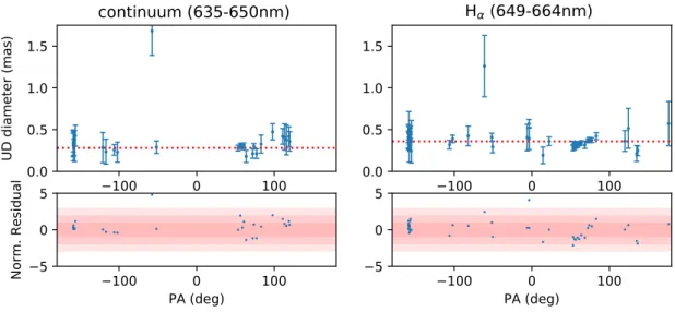
Fig. 3.Top panels: uniform disk diameter derived from each individual VEGA V2measurements (continuum band in the left and Hα band in the
right) plotted as a function of the baseline position angle (PA). The red dotted line represents the best-fit diameter from modeling all the data in each band (θ = 0.28 mas in the continuum and θ = 0.36 mas in the Hα band). Bottom panels: corresponding normalized residuals.
component similar to the one found from the continuum, that is, 0.26 ± 0.02 mas. The flux contribution of the second com-ponent and its extension are significantly constrained. However, the uncertainty remains quite large, that is, F2= 0.15 ± 0.03 and θ2= 6.5 ± 2.1 mas (see Table1).
Considering that the first component of our model repre-sents the stellar photosphere, our measurement is slightly higher than the value assumed in the work of Sigut et al. (2015) of 0.22 mas. However, their adoption for the stellar angular diam-eter is based on a spectral type-radius relation for B dwarf stars (Townsend et al. 2004). Moreover, this value of 0.22 mas rep-resents the polar radius. o Aquarii is a fast rotator likely to be significantly flattened, and our measurements are spread over dif-ferent orientations, so that we end up measuring a mean radius of the star projected on the sky. Assuming a distance of 144 pc (derived from the Gaia DR2 parallaxes, Gaia Collaboration 2018), θ1= 0.26 ± 0.02 mas corresponds to a stellar radius R?= 4.0 ± 0.3 R .
Finally, to try to detect any possible stellar or circumstel-lar disk flattening from the squared visibility measurements, we also computed individual uniform disk equivalent diameter for each V2measurement. This analysis of the uniform disk diame-ter for o Aquarii, as a function of the VEGA baseline orientation, is shown in Fig. 3. As expected from our analysis (consider-ing uniform elliptical models), we do not find any evidences of flattening from modeling our V2 dataset since no clear trends are found in the model residual as varying the baseline position angle.
4. Kinematic modeling: VEGA and AMBER differential data
To constrain the geometry and kinematics of the circumstellar gas in the Hα and Brγ lines, we fit the VEGA and AMBER differential visibility and phase measurements using a simple bi-dimensional kinematic model for a rotating disk4.
4.1. The kinematic model
This kinematic model was already used in a series of papers about spectro-interferometric modeling of Be stars, including
Delaa et al. (2011),Meilland et al. (2012), and Cochetti et al.
(2019), and is presented in detail in these references.
In short, the intensity map for the central star is modeled as a uniform disk, and the circumstellar disk as two elliptical Gaussian distributions, one for the flux in continuum, and the other one for the flux in line. The disk is geometrically thin so that the ellipse flattening ratio is set to 1/ cos i, where i is the inclination angle. The disk intensity map in the line is computed taking into account the Doppler effect due to the disk rotational velocity in the considered spectral channels. The parameters of our kinematic model are the following:
(i) The simulation parameters: size in pixels (nxy), field of view in stellar diameters ( f ov), number of wavelength points
4 Available at the JMMC service AMHRA: https://amhra.oca.
(nλ), central wavelength of the emission line (λ0), step size in wavelength (δλ), and spectral resolution (∆λ).
(ii) The global geometric parameters: stellar radius (R?), dis-tance (d), inclination angle (i), and disk major-axis position angle (PA).
(iii) The disk continuum parameters: disk major-axis FWHM in the continuum (ac), disk continuum flux normalized by the total continuum flux (Fc).
(iv) The disk emission line parameters: disk major-axis FWHM in the line (aline) and line equivalent width (EW).
(v) The kinematic parameters: rotational velocity (vrot) at 1.5 Rp (polar radius) and exponent of the rotational velocity power-law (β).
4.2. Model fitting using the MCMC method
To perform our model fitting, we used the code emcee ( Foreman-Mackey et al. 2013). This is an implementation in Python of the MCMC method from Goodman & Weare (2010). Some recent works on stellar interferometry used this code (see., e.g.,
Monnier et al. 2012; Domiciano de Souza et al. 2014, 2018;
Sanchez-Bermudez et al. 2017).
The simulation parameters were set as follows: nxy= 256, f ov = 60 D?, nλ= 60 (VEGA) and 110 (AMBER), λ0= 6563 Å (VEGA) and 21 661 Å (AMBER), δλ = 2.5 Å (VEGA) and 1.0 Å (AMBER), and ∆λ = 5.0 Å (VEGA) and 1.8 Å (AMBER). To reduce the number of free parameters, we set R?= 4.0 R and d = 144 pc. We also fixed the disk continuum extension acand flux Fcto 0 for VEGA (i.e., neglecting the disk contribution in the continuum, based on our analysis of the VEGA V2data). In the AMBER analysis, we adopted ac= 3 D? and Fc= 0.2 from
Cochetti et al.(2019). The line equivalent width was set to 19.9 Å in Hα (Sigut et al. 2015). For Brγ, we computed the EW using the AMBER spectra from all observations and found a mean value of 13.6 ± 1.1 Å, which is compatible with the value fromMeilland et al.(2012), 12.6 Å, but not with the result fromCochetti et al.
(2019) of 18.1 Å. Finally, from the ten parameters of the kine-matic model, the fitting of the VEGA and AMBER data were performed with at most five free parameters: i, PA, aline, vrot, and β.
The likelihood function (plike) of the MCMC procedure was chosen as ln(plike) = −χ2total/2, where χ2totalis the sum of the χ2 computed for the differential visibility and the differential phase. Thus, our attempt to converge to samples of parameters that maximizes the likelihood function means the minimization of the total χ2 between our interferometric data and the kinematic model.
We performed three different model fitting tests with differ-ent constraints on the value of vrot:
(i) Five free parameters: i, PA, aline, vrot, and β. Without the inclusion of any prior probability function in the analysis.
(ii) Four free parameters: i, PA, aline, and β. The stellar rota-tional velocity vrot is fixed on the critical value of 391 km s−1 (Frémat et al. 2005).
(iii) Five free parameters: i, PA, aline, vrot, and β. We take into account a prior probability function pprioron v sin i. Adopting µ = 282 km s−1 and σ = 20 km s−1, from the measured v sin i = 282 ± 20 km s−1 (Frémat et al. 2005), we have the following expression for pprior:
ln(pprior) = −(v sin i − µ)
2
2σ2 , (1)
where v sin i is calculated from the sampled MCMC values for the stellar rotational velocity and inclination angle.
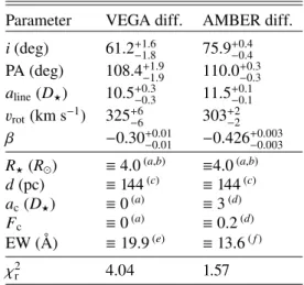
Table 2. Best-fit kinematic models from test (iii) for our VEGA (Hα) and AMBER (Brγ) differential data.
Parameter VEGA diff. AMBER diff.
i (deg) 61.2+1.6 −1.8 75.9+0.4−0.4 PA (deg) 108.4+1.9 −1.9 110.0+−0.30.3 aline(D?) 10.5+−0.30.3 11.5+−0.10.1 vrot(km s−1) 325+6−6 303+2−2 β −0.30+0.01 −0.01 −0.426+−0.0030.003 R?(R ) ≡ 4.0(a,b) ≡4.0(a,b) d (pc) ≡ 144(c) ≡ 144(c) ac(D?) ≡ 0(a) ≡ 3(d) Fc ≡ 0(a) ≡ 0.2(d) EW (Å) ≡ 19.9(e) ≡ 13.6( f ) χ2r 4.04 1.57
Notes. We show the median and the first and third quartiles for each parameter derived from the MCMC analysis. Adopted parameters stand
by “≡”.(a)Based on our fit to the VEGA squared visibility.(b)Radius
derived considering the distance adopted from Gaia Collaboration
(2018).(c)Distance adopted fromGaia Collaboration(2018).(d)Adopted
from Cochetti et al. (2019). (e)Adopted from Sigut et al. (2015).
( f )Measured from our AMBER observations.
Hence, considering a high weight on pprior, the following quantity for the posterior probability function ppost is maxi-mized: ln(ppost) = − 100 (v sin i − µ) 2 2σ2 ! −χ22. (2)
Note that this is equivalent to the case of equal weights for pprior and plike, but considering a lower error bar on v sin i, namely, σ = 2 km s−1.
We typically used several hundreds of walkers (∼300–900) for the MCMC run. Convergence was obtained for about 50 to 100 iteration steps in each walker, but we used a conservative value of 150 steps in the burn-in phase and 50 in the main phase to estimate the parameters values and uncertainties. Overall, we found a mean acceptance fraction of ∼0.5–0.6 in our MCMC tests. This is close to the optimal range for this parameter of ∼0.2–0.5 (see, e.g.,Foreman-Mackey et al. 2013).
4.3. Best-fits in Hα and Brγ
We modeled a total of 117 (VEGA) and 24 (AMBER) measure-ments of differential visibility and phase. The best-fit parameters for the MCMC fit with a prior on v sin i (test iii, described above) are presented in Table2. The corresponding histograms and the two-by-two parameter correlations from this MCMC run (one for VEGA and other for AMBER) are shown in Fig.4. The corre-sponding histograms and correlation plots for the other two fits (tests i and ii) are shown in Figs.B.1andB.2. One sees that the values of i, PA, and aline, derived from each emission line, differ only marginally in all the fitting tests, showing the robustness of the solution for these parameters.
In Fig.5, we show examples of VEGA and AMBER data in comparison to our best-fit kinematic models. For later discus-sion in Sect.6, the visibility and phase from our best-fit HDUST model is also presented here. Our best-fit kinematic models are able to reproduce both the VEGA and AMBER differential data
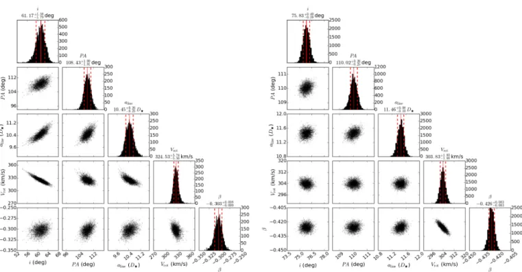
Fig. 4.Histogram distributions and two-by-two correlations (after the burn-in phase) for the free parameters of our best-fit kinematic models using MCMC for the VEGA (left panel) and AMBER (right panel) differential data. The median values are shown in solid red lines and the first and third quartiles in dashed red lines. The median and the first and third quartiles estimated for the parameters of our best-fit models (VEGA and AMBER)
are presented in Table2. In the correlation plots, darker points correspond to models with lower values of χ2. See text for discussion.
λ (nm) Vd if f 654.8 656.0 657.2 0.3 0.6 0.9 λ (nm) φd if f (deg) 654.8 656.0 657.2 -40 -10 20 λ (nm) Vd if f 654.8 656.0 657.2 0.3 0.6 0.9 λ (nm) φd if f (deg) 654.8 656.0 657.2 -40 -10 20 λ (nm) Vd if f 2164.0 2165.6 2167.2 0.7 0.9 λ (nm) φd if f (deg) 2164.0 2165.6 2167.2 -30 0 20 λ (nm) Vd if f 2164.0 2165.6 2167.2 0.7 0.9 λ (nm) φd if f (deg) 2164.0 2165.6 2167.2 -30 0 20
Fig. 5.Comparison between our best-fit kinematic models (dashed red; Table2) and two different VEGA (top panels) and AMBER (bottom panels)
measurements (black line). Our best-fit HDUST model is also shown (dashed blue; Table5; discussion in Sect.6). δλ of the kinematic model and
AMBER data is increased to 1.8 Å in order to compare them to the HDUST model (δλ fixed to 1.8 Å).
well. We found a reduced χ2 of ∼4.0 and 1.6 from fitting, in a separate way, respectively, the VEGA and AMBER datasets.
We derived compatible values for the disk PA (∼110◦) from fitting the VEGA and AMBER data with an uncertainty up to ∼2◦. This result agrees well with previous studies (e.g.,Meilland
et al. 2012;Touhami et al. 2013;Sigut et al. 2015;Cochetti et al. 2019). On the other hand, the inclination angle determined from the fit to the VEGA data is significantly smaller (i = 61.2 ± 1.8◦) in comparison to the one determined from fitting AMBER (i = 75.9 ± 0.4◦). This latter value is in good agreement with the results for i found by Meilland et al.(2012) andCochetti et al.
(2019). We also constrain the disk extension with a good preci-sion: aline= 10.5 ± 0.3 D?in the Hα line and aline= 11.5 ± 0.1 D?
in the Brγ line. These values are compatible with the ones deter-mined bySigut et al.(2015) in Hα andMeilland et al.(2012) in Brγ.
Another aspect concerning the disk extension in Brγ is the significant discrepancy seen in comparison to aline= 8.0 ± 0.5 D? fromCochetti et al.(2019). However, these authors used a larger value for the stellar radius of 4.4 R and a closer distance of 134 pc (van Leeuwen 2007), having thus the angular size of the stellar diameter larger in ∼19% than the one assumed in our kine-matic analysis from our results in Sect.3. Considering all the other parameters fixed, this results in a smaller disk extension in ∼19% than one found from our analysis. Nevertheless, the largest contribution to this discrepancy between our results and the ones
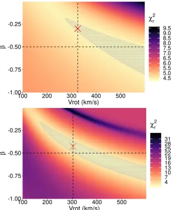
-1.00 -0.75 -0.50 -0.25 100 200 300 400 500 Vrot (km/s) β 4.5 5.0 5.5 6.0 6.5 7.0 7.5 8.0 8.5 9.0 9.5 χr2 -1.00 -0.75 -0.50 -0.25 100 200 300 400 500 Vrot (km/s) β 4 7 10 13 16 19 22 25 28 31 χr2
Fig. 6.χ2r maps of 40 000 kinematic models as a function of vrotand
βfrom the fit to VEGA (top panel) and AMBER (bottom panel)
dif-ferential data. Only these two parameters were varied in a regular step
in the intervals shown here. The other parameters are fixed (Table2).
Our results found from the MCMC analysis for vrotand β are indicated
with red crosses. In order to highlight the correlation between β and vrot,
the gray region corresponds to an arbitrary number of models, encom-passing about the 5000 best models in both cases. The value of β = −0.5
(Keplerian disk) and our determination for vrotare marked in dashed
black line. Note the strong correlation between the stellar rotational velocity and the disk velocity law exponent in both the cases. Also, note that a Keplerian disk is found from modeling the AMBER data, but not from VEGA.
fromCochetti et al.(2019) is due to their high value of equiva-lent width in the Brγ line of 18.1 Å, as discussed in Sect.4.2, that also implies in a smaller disk extension in this line.
From our various tests, we showed that β and vrotare strongly correlated. To precisely determine their dependence, we com-puted a grid of kinematic models varying just these two parame-ters in a regular step size. The values for i, PA, alineare fixed from Table2. The resulting χ2
r maps are shown in Fig.6. As expected, one sees that vrotand β are highly correlated for the VEGA and AMBER data. This high degeneracy can be understood since these two parameters provide the rotational velocity structure in the disk: it is hard to distinguish the effects of each one on the modeling of spectro-interferometric (and spectroscopic) data.
Furthermore, we see that β = −0.5 (Keplerian disk) pro-vides unrealistically high values for the stellar rotational velocity ((&)400 km s−1; gray region) of o Aquarii (VEGA analysis). For AMBER, vrotis significantly reduced to about 300–400 km s−1. As shown in Fig.6, our results from AMBER are consistent with a nearly Keplerian rotating disk (β ∼ 0.43). However, it is con-spicuous that the β value calculated from the VEGA data (β ∼ 0.30) shows such a large departure from the Keplerian case.
Cochetti et al.(2019) derived a stellar rotational velocity of 355 ± 50 km s−1and β = −0.45 ± 0.03. This is in fair agreement
with our results for both vrotand β. Considering our MCMC test (ii), where vrotis fixed to the critical value and β is a free param-eter, the results for β are shifted to higher values (more positive) with β ∼ −0.42 (VEGA) and −0.54 (AMBER).
Therefore, regardless the MCMC fitting considered here, we verify a discrepancy of about 0.1 between the value of β derived from the Hα and Brγ lines. Our results from the AMBER analy-sis (Brγ) seems to be conanaly-sistent with a nearly Keplerian rotating disk, but we verified a larger departure from β = −0.5 for the VEGA analysis (Hα).
5. Radiative transfer modeling
5.1. The code HDUST
We used the 3D non-LTE radiative transfer code HDUST5
(Carciofi & Bjorkman 2006,2008) to perform a deeper physi-cal analysis of o Aquarii. In addition to geometric and kinematic parameters, we seek to derive the density and temperature distri-butions in the disk, and the spectral energy distribution (SED), none of which was provided by the two simpler models con-sidered in the two previous sections. HDUST uses a Monte Carlo method to solve the radiative transfer, statistical and radia-tive equilibrium equations for arbitrary density and velocity distributions in gaseous (pure hydrogen) or dusty circumstellar environments.
This code is well-suited to model the circumstellar environ-ment of Be stars as it impleenviron-ments the VDD model. Thus, the disk velocity law is assumed to be Keplerian (β fixed to −0.5). Many previous studies explored formal solutions of the VDD model in several limiting cases. For example,Bjorkman & Carciofi(2005) investigated the isothermal, steady-state case of a disk formed by a steady mass injection rate over a long time. Effects due to non-isothermal temperature structure were studied byCarciofi & Bjorkman (2008). Haubois et al. (2012) studied the temporal evolution of the disk structure that is subject to variable mass inject rates. Finally, the effects of a binary companion on the disk were studied byOkazaki et al.(2002),Oudmaijer & Parr(2010),
Panoglou et al.(2016), andCyr et al.(2017), among others. From these studies, the radial density profile in Be star disks is found to be quite complex, for example, depending on the disk age, dynamical state, or presence of a binary companion. Despite this complexity, several studies have shown that the global behavior of this density profile is successfully approximated by a simple radial power-law (e.g.,Touhami et al. 2009;Vieira et al. 2017). Considering also that the vertical density structure is that of an isothermal disk (hydrostatic assumption in the z-axis), the disk density can be parameterized as follows:
ρ(r, z) = ρ0 Rreq !m exp −z2 2H(r)2 ! , (3)
where ρ0is the disk base density, Reqis the equatorial radius, and H(r) is the (isothermal) disk scale height given by:
H(r) = H0 Rr eq
!3/2
, (4)
and H0is the scale height at the disk base, H0=csReq GMR ?
eq !−1/2
, (5)
5 For access and collaborations with HDUST, please contact A. C.
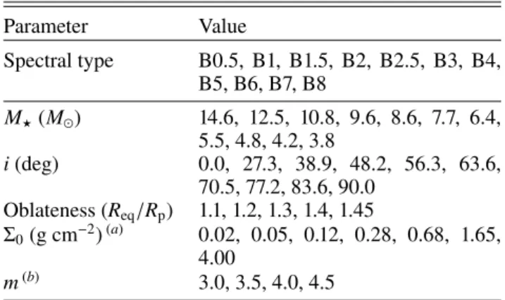
Table 3. HDUST parameters in the BeAtlas grid. Parameter Value Spectral type B0.5, B1, B1.5, B2, B2.5, B3, B4, B5, B6, B7, B8 M?(M ) 14.6, 12.5, 10.8, 9.6, 8.6, 7.7, 6.4, 5.5, 4.8, 4.2, 3.8 i (deg) 0.0, 27.3, 38.9, 48.2, 56.3, 63.6, 70.5, 77.2, 83.6, 90.0 Oblateness (Req/Rp) 1.1, 1.2, 1.3, 1.4, 1.45 Σ0(g cm−2)(a) 0.02, 0.05, 0.12, 0.28, 0.68, 1.65, 4.00 m(b) 3.0, 3.5, 4.0, 4.5
Notes. First row indicates the spectral type corresponding to the stellar
mass (Townsend et al. 2004). Models are calculated with the
follow-ing fixed parameters: fraction of H in the core Xc= 0.30, metallicity
Z = 0.014, and disk radius = 50 Req.(a)Surface density at the base of the
disk.(b)Disk mass density law exponent.
where M?is the stellar mass, G the gravitational constant, and cs the sound speed velocity which depends on the local disk temperature T:
cs= s
kBT
µmH, (6)
where kB is the Boltzmann constant, µ is the mean molecular weight of the gas, mH is the hydrogen mass, and T is adopted as 0.72Tpol, where Tpol is the polar effective temperature (see
Correia Mota 2019).
HDUST has been used a few times to model spectro-interferometric observations (e.g.,Carciofi et al. 2009;Klement et al. 2015;Faes 2015). From the solution of the radiative transfer problem, we are able to calculate synthetic spectra and intensity maps as a function of the wavelength around specific spectral lines. We estimated the stellar and circumstellar disk parameters from the comparison of our spectro-interferometric observations (visible and near-infrared) with synthetic observables computed from the Fourier transform of HDUST monochromatic intensity maps.
5.2. BeAtlas grid
Since a few hours are needed to compute a single HDUST model, it is not possible to perform an iterative model fitting procedure similar to the one described in Sect.4. To overcome this issue, we used a pre-computed grid of HDUST models called BeAtlas (Faes 2015;Correia Mota 2019). The BeAtlas grid is presented and described in detail by these references. It consists of ∼14 000 models with images (specific intensity maps), SEDs, and spectra calculated in natural and polarized spectra, over several spectral regions, including the Hα and Brγ lines that are of interest for the analysis of our VEGA and AMBER dataset.
In Table3, we show the parameter space covered by BeAtlas. Five physical parameters are varying in the grid. The stellar mass M?, the inclination angle i, and the stellar oblateness Req/Rp, fully describe the star. Other stellar parameters such as the stellar polar radius (Rp), rotational velocity (vrot) and linear and angular rotational rates (vrot/vcritand Ω/Ωcrit) can be computed from M? and Req/Rpassuming rigid rotation under the Roche model (see, e.g., Carciofi & Bjorkman 2008). The two last parameters in
Table3describe the circumstellar disk structure and are parame-terizations of the VDD model: the base surface density (Σ0) and the radial density exponent (m).
The previously described volume mass density (Eq. (3)) and the surface mass density are related as follows:
Σ(r) ≡ Z +∞ −∞ ρ(r, z)dz, (7) ρ(r, z) = Σ(r) H(r)√2πexp −z2 2H(r)2 ! . (8)
From that, to facilitate the comparison to other disk models, we note that the relation between the volume and surface mass densities at the base of the disk is given by:
ρ0= Σ0 s
GM?
2πcs2Req3. (9)
The range of values for Σ0 and m in the grid encompasses somewhat extreme cases in the literature for the circumstellar disk of Be stars. For example, see Fig. 7 ofVieira et al.(2017). The listed values of Σ0correspond to ρ0from ∼10−12g cm−3to ∼10−10g cm−3. Parametric models with m = 3.5 are equivalent to the steady-state solution of the viscous diffusion equation con-sidering an isothermal disk scale height. Thus, concerning the mass density law exponent m, models with m > 3.5 would rep-resent a disk in an accretion phase, while the ones with m < 3.5 a disk in an ongoing process of dissipation (see, e.g.,Haubois et al. 2012;Vieira et al. 2017).
5.3. Results
We performed four different analyses of our data using different subsets. For that, the reduced χ2between the predicted interfer-ometric observables from each HDUST model and the data was calculated as follows:
(i) calibrated VEGA V2 in the 642.5 nm band (close-by continuum to Hα).
(ii) VEGA differential visibility and phase (Hα line). (iii) AMBER differential visibility and phase (Brγ line). (iv) All the quantities above analyzed together.
Analysis (i) was performed to evaluate the constraint on the stellar mass M? and oblateness Req/Rp. In Fig. 7, we show the lowest value of χ2
r for each value of stellar oblateness and mass from fitting the VEGA V2data in the continuum band. The pre-dicted V2 from our best-fit BeAtlas model (with M
?= 4.2 M ; Table5) is overplotted to the VEGA measurements. For compar-ison, the predicted visibility curve from the BeAtlas model with the highest stellar mass, M?= 14.6 M , is also overplotted to the data. These two models have the same values of i, Req/Rp, Σ0, and m. In Sect.3, we presented a similar analysis, but in terms of simple geometric models. For better visualisation, we show in Fig.7the local regression fits of χ2
r as a function of Req/Rpand M?. Like all such calculations in this paper, all these regression fits of χ2
r are performed with the LOESS method6.
As in the analysis with geometric models, we cannot con-strain the stellar oblateness using VEGA V2 data. On the other hand, the mass is better constrained with M?∼ 4.8 M (B6 dwarf). From Fig. 7, one sees how the measured V2 are mismatched by the HDUST model with M?= 14.6 M (unreal-istic mass value for o Aquarii) due to the larger polar radius of
6 As implemented in R: https://stat.ethz.ch/R-manual/
4.0 4.5 5.0 5.5 6.0 6.5 7.0 7.5 8.0 8.5 9.0 9.5 10.0 1.10 1.20 1.30 1.40 1.45 Req Rp Lo w es t χr 2 4.0 4.5 5.0 5.5 6.0 6.5 7.0 7.5 8.0 8.5 9.0 9.5 10.0 3.8 4.2 4.8 5.5 6.4 7.7 8.6 9.6 10.8 12.5 14.6 Stellar mass (M☉) Lo w es t χr 2 0.00 0.25 0.50 0.75 1.00 1.25
1e+08 2e+08 3e+08 4e+08
Spatial freq. (1/rad)
V
2
Fig. 7.Analysis (i): lowest value of reduced χ2 (χ2
r) for each value of Req/Rp (left panel) and stellar mass (middle panel) from the HDUST fit to
the VEGA V2data (642.5 nm band). Local regression fits to χ2
r, as a function of the parameter values, are shown in red line. In the right panel,
the predicted visibility from our best-fit HDUST model (red points; Table5) is compared to the VEGA V2measurements in the continuum band
(black points). The predicted visibility from the HDUST model with the highest mass in the BeAtlas grid (14.6 M , highest χ2rin the middle panel)
is shown in blue points.
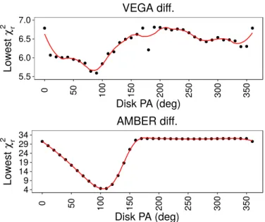
5.5 6.0 6.5 7.0 0 50 100 150 200 250 300 350 Disk PA (deg) Lo w es t χ r 2 VEGA diff. 4 9 14 19 24 29 34 0 50 100 150 200 250 300 350 Disk PA (deg) Lo w es t χ r 2 AMBER diff.
Fig. 8.Lowest value of χ2
r for each value of disk major-axis position
angle from the HDUST fit to the VEGA (top panel, analysis (ii)) and AMBER (bottom panel, analysis (iii)) differential visibility and phase.
Local regression fits of χ2
r as a function of the disk PA are shown as a
red line.
∼7.4 R in this model. Among all the values for M?in the grid, M?= 4.2 M corresponds to a B7 dwarf star (Townsend et al.
2004). Since o Aquarii shows luminosity class III-IV, it could be expected to have a mass somewhat higher than a dwarf of same spectral type, which is compatible with our results.
In Fig.8, we show the lowest χ2
r for each value of disk major-axis position angle PA from the fit to the VEGA and AMBER differential visibilities and phases: analyses (ii) and (iii). Here, the stellar mass is fixed to M?= 4.2 M from analysis (i), which also allows a better comparison to other studies of o Aquarii (e.g.
Sigut et al. 2015). In both cases, χ2
r of the models is minimized around PA = 110◦, a value that we adopt in the remaining of this section. This is in good agreement to our results found with the kinematic model in Sect.4.
In Fig.9, we present our results from modeling the VEGA and AMBER differential visibility and phase in a separate way – analyses (ii) and (iii) – as well as from the simultaneous fit to all the interferometric data (analysis (iv)). The lowest χ2
r is shown as a function of the following HDUST parameters: the inclination angle, stellar oblateness, base disk surface density, and the radial disk density law exponent. In Table4, we show the statistics from these parameters calculated from the HDUST models within a certain threshold of χ2
r, which, in each case, is chosen to match a similar number of models (∼15–20 best-models). In Table4, the parameters for the models with the lowest value of χ2
r are also shown. In Table5, we show the parameters for the best BeAtlas model to explain simultaneously all our different interferometric datasets.
Since our HDUST analysis is limited to the pre-computed BeAtlas grid (limited parameter space and selected parameter values), we stress that the results presented here do not corre-spond to the real χ2 minimum to explain our datasets in the framework of HDUST. Furthermore, the values for the standard deviation are shown in parenthesis in Table4since these are not determinations for the error bars on the parameters. They are just an evaluation for the dispersion on the parameters values of the BeAtlas best-models (within in a certain threshold of χ2
r). For example, from fitting AMBER, we found that all the BeAtlas models have Σ0= 0.12 g cm−2, and m = 3.0, up to, respectively, the top 207% and top 240% best-models. For this reason, it is shown, in this case, null standard deviation in Table4for these parameters (top 54% best-models).
From the separate analysis of the VEGA and AMBER dif-ferential datasets, we are able to describe the stellar and disk parameters, in Hα and Brγ, by the same HDUST model with: Req/Rp= 1.45, Σ0= 0.12 g cm−2, and m = 3.0. One clear excep-tion is found for the inclinaexcep-tion angle. From the Hα analysis, χ2 r is minimized for i = 56.3◦. On the other hand, this is achieved with i = 77.2◦ in the Brγ line. Such discrepancy of ∼20◦ is in agreement with the one found from our kinematic modeling. As expected, the joint analysis to all the data provides an inter-mediate mean value of ∼65◦for the inclination angle, showing a larger dispersion (higher standard deviation) in comparison to the results found from the separate analysis for VEGA and
6 7 8 0.0 27.3 38.9 48.2 56.3 63.6 70.5 77.2 83.6 90.0 i (deg) Lo w es t χr 2 6.0 6.2 6.4 6.6 6.8 1.10 1.20 1.30 1.40 1.45 Req Rp 6.0 6.5 7.0 0.02 0.05 0.12 Σ0 (g cm2) 6.0 6.5 7.0 7.5 8.0 3.0 3.5 4.0 4.5 m 10 20 30 0.0 27.3 38.9 48.2 56.3 63.6 70.5 77.2 83.6 90.0 i (deg) Lo w es t χr 2 4 6 8 10 1.10 1.20 1.30 1.40 1.45 Req Rp 5 10 15 20 0.02 0.05 0.12 Σ0 (g cm 2 ) 10 20 3.0 3.5 4.0 4.5 m 7.5 10.0 12.5 15.0 0.0 27.3 38.9 48.2 56.3 63.6 70.5 77.2 83.6 90.0 i (deg) Lo w es t χr 2 6.5 7.0 7.5 8.0 1.10 1.20 1.30 1.40 1.45 Req Rp 6 8 10 0.02 0.05 0.12 Σ0 (g cm2) 6 8 10 12 14 3.0 3.5 4.0 4.5 m
Fig. 9.Lowest value of χ2
r for each value of stellar inclination angle, oblateness, base disk surface density, and disk density law exponent from
the HDUST fit to the: VEGA differential data (top, analysis (ii)), AMBER differential data (middle, analysis (iii)), and all the interferometric data
considered in this section (bottom panel, analysis (iv)). The stellar mass is fixed to 4.2 M and disk PA to 110◦. Local regression fits to χ2r, as a
function of the parameter values, are shown as a red line. The mean parameter values for the sets of best models (Table4) are marked in dashed
black line. Our best-fit BeAtlas model to fit all the interferometric data is shown in Table5. See text for discussion.
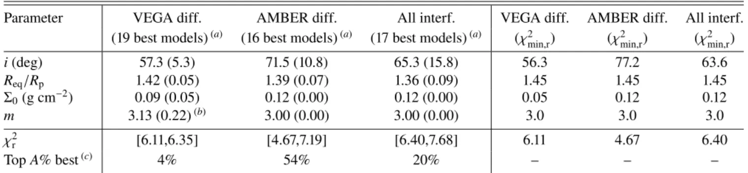
Table 4. First three columns: mean and standard deviation values for each HDUST parameter of the BeAtlas grid: from analysis (ii) (19 best-fit HDUST models), analysis (iii) (16 best-fit HDUST models), and analysis (iv) (17 best-fit HDUST models).
Parameter VEGA diff. AMBER diff. All interf. VEGA diff. AMBER diff. All interf.
(19 best models)(a) (16 best models)(a) (17 best models)(a) (χ2
min,r) (χ2min,r) (χ2min,r)
i (deg) 57.3 (5.3) 71.5 (10.8) 65.3 (15.8) 56.3 77.2 63.6 Req/Rp 1.42 (0.05) 1.39 (0.07) 1.36 (0.09) 1.45 1.45 1.45 Σ0(g cm−2) 0.09 (0.05) 0.12 (0.00) 0.12 (0.00) 0.05 0.12 0.12 m 3.13 (0.22)(b) 3.00 (0.00) 3.00 (0.00) 3.0 3.0 3.0 χ2r [6.11,6.35] [4.67,7.19] [6.40,7.68] 6.11 4.67 6.40 Top A% best(c) 4% 54% 20% – – –
Notes. In the bottom rows, there are shown the intervals of χ2
r between the minimum value χ2min,rand a certain threshold A (χ2min,r+ A%). From
modeling the AMBER data, all models have Σ0= 0.12 g cm−2and m = 3.0 up to, respectively, χ2min,r+ 207% and 240%, thus the standard deviation
shown here is null. The parameters of the HDUST models with χ2
min,rare given in the last three columns. The stellar mass is fixed to 4.2 M and
disk PA = 110◦.(a)These values of standard deviation are given in parenthesis since they are not error bars on the parameters.(b)Mean and standard
deviation calculated from 16 models since three out of 19 models, in this χ2
r threshold, are non-parametric models of the BeAtlas grid.(c)“Top A%
best” stands by the HDUST models with χ2
min,r≤ χ2r ≤ χ2min,r+ A%, where χ2min,ris the minimum χ2r. These thresholds are chosen to encompass
about the same number of HDUST models (∼15–20 models).
Table 5. Parameters of our best-fit HDUST model in the BeAtlas grid to explain the joint analysis of our interferometric data: VEGA calibrated and differential data and AMBER differential data.
M?(M ) Req/Rp i (deg) PA (deg) Σ0(g cm−2) m Rp(R ) vrot(km s−1) vrot/vcrit
4.2 1.45 63.6 110 0.12 3.0 3.7 368 0.96
Notes. A part of these parameter values are presented in the last column of Table4. The polar radius and the stellar rotational velocity are obtained
1 mas N E Continuum = 654.3 nm HDUST model N E 1 mas Kinematic model H line ( =2.7nm) = 656.3 nm = 656.1 nm v = -118.0 km/s = 656.3 nm v = -59.0 km/s = 656.4 nm v = 0.0 km/s = 656.5 nm Narrow-band Maps through the H line ( =0.12nm)
v = 59.0 km/s = 656.7 nm v = 118.0 km/s = 656.8 nm v = 176.0 km/s 0.000 0.017 0.101 0.278 0.572 1.000
Flux per pixel (arbitrary unit)
1 mas N E Continuum = 2161.2 nm HDUST model N E 1 mas Kinematic model Br line ( =3.9nm) = 2166.1 nm = 2.1651 m v = -135.0 km/s = 2.1656 m v = -61.0 km/s = 2.1661 m v = 12.0 km/s = 2.1666 m Narrow-band Maps through the Br line ( =0.15nm)
v = 86.0 km/s = 2.1672 m v = 160.0 km/s = 2.1677 m v = 233.0 km/s 0.000 0.017 0.101 0.278 0.572 1.000
Flux per pixel (arbitrary unit)
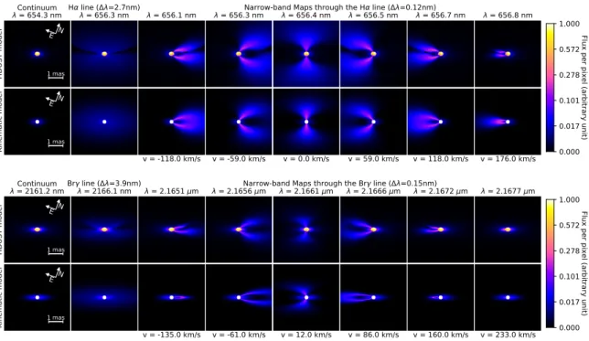
Fig. 10.Intensity maps of our best-fit HDUST and kinematic models at different wavelengths around the Hα line (first two rows) and the Brγ line (last two rows). Flux/pixel is in arbitrary units with the same scale in Hα and Brγ. The image integrated in wavelength around each of these lines (∆λ = 2.7 nm around Hα and 3.9 nm around Brγ) are shown in the second column.
AMBER. One sees that the mean value for stellar oblateness is somewhat decreased, when considering all the datasets. How-ever, in this case, the dispersion is significantly increased (±0.09) when compared to the separate VEGA and AMBER differential fits (±0.05–0.07). This happens due to the inclusion of the cal-ibrated VEGA data in the joint analysis that do not allow us to properly infer this parameter (see, again, Fig.7).
6. Comparison between kinematic and HDUST best-fit models
In Fig. 5, we compare the synthetic differential visibility and phase from our best-fit kinematic and HDUST models to the actual VEGA and AMBER data for a few baselines. Compar-isons to non-interferometric observables (spectral energy distri-bution and line profiles) are presented in Sect. 7. Our best-fit models are compared to all the AMBER data in Fig.C.1. One sees that our best-fit kinematic models do a better job of repro-ducing both the VEGA and AMBER data. From the separate kinematic modeling of the VEGA and AMBER differential data, the χ2
r of the model is lower than with HDUST (BeAtlas grid). Fixing the stellar mass to a reliable value for o Aquarii (4.2 M ), our best-fit HDUST model has χ2
r ∼ 6.1 and 4.7 for VEGA and AMBER, respectively. From the kinematic modeling, we found χ2r ∼ 4.0 and 1.6 to explain these same datasets.
For VEGA, in particular, our best-fit HDUST model adjust-ment for the measured visibility width is worse than with the kinematic model. This particular issue in modeling the VEGA data can be explained; in HDUST, the disk velocity law expo-nent is fixed by β = −0.5 (Keplerian disk rotation), while in the kinematic model it is a free parameter. As shown in Sect.4.3, we find values for β that are higher than −0.5, and this is accentuated from the analysis of the VEGA data (β ∼ −0.3).
Apart from this issue regarding the analysis in Hα, we are able to describe well the disk density with the same physical
parameters in both the Hα and Brγ lines: Σ0= 0.12 g cm−2 and m = 3.0. As will be later discussed, this result found using HDUST is consistent with the ones presented in Sect. 4.3, showing a similar disk extension in these lines.
In Fig. 10, the intensity maps for each model are shown at the close-by continuum region and at different wavelength values in both the Hα and Brγ emission lines. The integrated intensity map (around each of these lines) is also presented. For a more realistic comparison, here we consider our best-fit kinematic model with a small flux contribution of 5% from the disk in the continuum nearby to Hα and ac= 2 D?. As shown in Table2, these parameters were adopted as null in the kinematic analysis for the VEGA data, since we were not able to resolve the disk from our analysis of VEGA V2measurements in the continuum band (Sect.3). Regarding the continuum region close to Brγ, the disk extension and flux contribution are given in Table2for the AMBER analysis.
The major difference between the intensity maps in Hα and Brγ is the disk flattening which is due to the different inclina-tion angle derived from these two regions, i ∼57◦(Hα) and ∼72◦ (Brγ), from the best models provided in Table4. Moreover, as seen in the images, the stellar flattening is taken into account in the HDUST modeling, but not in the kinematic model (the star is modeled as a uniform disk). Apart from these departures, we see that our best-fit HDUST model presents a fairly similar distribu-tion to the one computed with the kinematic code: a Gaussian distribution represents the circumstellar disk. This can be better noted considering the full integrated images around the emission lines.
7. Comparison to non-interferometric observables
In this section, we compare our best-fit models, found from the analysis of interferometric observables, to the observed spec-tral energy distribution (SED) and line profiles (Hα and Brγ)
λ (µm) log
(
Fλ)
0.145 0.245 0.345 0.445 0.545 -10.5 -10.1 -9.7 -9.3 λ (µm) log(
Fλ)
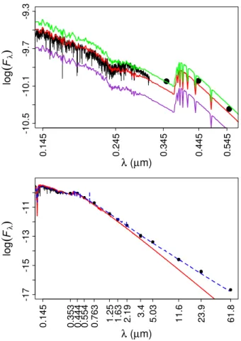
0.145 0.353 0.444 0.554 0.763 1.25 1.63 2.19 3.4 5.03 11.6 23.9 61.8 -17 -15 -13 -11Fig. 11. Comparison between the observed o Aquarii and model SEDs from the ultraviolet to the far-infrared region. Flux unit is
in erg cm−2 s−1 Å−1 and wavelength is shown in logarithmic scale.
IUE/SWP and IUE/LWP spectra are shown in black line and photo-metric data in black points. Top panel: purely photospheric models (color lines) with variation in the stellar radius (no inclusion of
geo-metrical oblateness): R?= 3.2 R (orchid), 4.0 R (red), and 4.4 R
(green). Bottom panel: photospheric model with 4.0 R (red) and our
best-fit HDUST model from fitting all the interferometric data (dashed
blue line; Table5). Note that the UBV-bands are better reproduced with
R?= 4.0–4.4 R . Our best HDUST model reproduces the observed IR
excess due to the circumstellar disk well.
of o Aquarii. With respect to polarimetric data, it is discussed in Sect.8.4.3when addressing the disk stability.
7.1. Spectral energy distribution
In Fig.11, we present the spectral energy distribution (SED) of o Aquarii from the ultraviolet (IUE/SWP and IUE/LWP spectra7)
to the far-infrared region. References for the photometric data are given as follows: UBVJHK-bands (Anderson & Francis 2012), i-band (Henden et al. 2016), LM-bands (Bourges et al. 2017), and IRAS 12, 25, and 60 µm bands (Abrahamyan et al. 2015).
For the spectral region up to the V-band, we compare the data to the SEDs of purely photospheric atmosphere models with solar metallicity (Castelli & Kurucz 2004). In this region, the circumstellar disk flux level is much lower than the photo-spheric flux, thus allowing a proper probe of the stellar radius (e.g., Meilland et al. 2009). The surface gravity was fixed at log g = 4.0, this being the closest value in Castelli & Kurucz
(2004) to log g = 3.9 that is given by our results of M?= 4.2 M
7 Public data available in the Barbara A. Mikulski Archive for Space
Telescopes (MAST):https://archive.stsci.edu/iue/
and R?= 4.0 R . The effective temperature was fixed at 13 000 K, followingCochetti et al.(2019). As in the previous sections, we consider the distance to be 144 pc, from the Gaia DR2 parallax. These synthetic SEDs were calculated for three different stel-lar radius values, R?: 3.2 R (Sigut et al. 2015), 4.0 R , and 4.4 R (Cochetti et al. 2019). The value of 4.0 R corresponds to the stellar radius determined from the fit to the VEGA V2 data using a two-component model: 4.0 ± 0.3 R . The effect of interstellar medium extinction is not included in these models since it is negligible for o Aquarii. Assuming a total to selective extinction ratio of RV= 3.1,Touhami et al.(2013) derived a color excess of E(B−V) = 0.015 ± 0.008 for this star from their fit to the SED. This means the observed flux is ∼96% of the intrinsic one in the V-band (lower by ∼0.02 dex). It is beyond the scope of this paper to estimate the extinction due to the circumstel-lar disk, however, from the comparison to purely photospheric models, we see in Fig.11that the effect of extinction (due to the interstellar and circumstellar matter) is conspicuously weak on the 0.220 µm bump.
From Fig. 11, we see that the UV and visible regions are better reproduced for a stellar radius of about 4.0–4.4 R , when compared to 3.2 R , adopted inSigut et al.(2015), which corre-sponds to the expected polar radius for a B7 dwarf. We stress that the radius derived byCochetti et al.(2019) is closer to our results from the fit to the VEGA V2data (Sect.3). Their result of R
?=
4.4 R corresponds to a uniform disk diameter of θ ∼ 0.28 mas (d = 144 pc). A better comparison toCochetti et al.(2019) is hard since they do not provide error bars on R?from fitting the SED. Furthermore, they derived R?= 4.4 R for o Aquarii using a dis-tance of 134 pc fromvan Leeuwen(2007), rather than the value of 144 pc adopted here. From Fig.11, this implies a larger dis-crepancy between the observed and synthetic SED for R?= 4.4 R , overestimating the observed flux.
We also compare the predicted SED of our best-fit HDUST model (Table5) to the SED of the purely photospheric model with 4.0 R . Despite being able to reproduce the UBV-bands well, one sees that a purely photospheric model clearly under-estimates the observed flux beyond the near-infrared due to the flux contribution from the circumstellar disk (e.g.,Poeckert & Marlborough 1978; Waters 1986). From Fig. 11, it is evident that the SED is much better reproduced up to the far-infrared region when taking into account the IR excess from the gaseous circumstellar disk present in our best-fit HDUST model. 7.2. Hα and Brγ profiles
Our Hα spectra taken with the VEGA instrument (20 spectra, period from 2012 to 2016) are not analyzed in this work since they are saturated. This is a known effect seen in previous works on Be stars and correlated to the magnitude of the object. We stress that this instrumental saturation effect does not impact the visibilities and phases extracted from the fringes measured with VEGA (see, e.g.,Delaa et al. 2011). To overcome this problem we used Hα line profiles from the BeSOS8catalog (Arcos et al.
2018;Vanzi et al. 2012), obtained between 2012 and 2015, and thus covering a similar period to our VEGA observations. The typical spectral resolution of the BeSOS spectra is ∼0.1 Å.
In Fig. 12, we compare the Hα and Brγ profiles from our best-fit models to observed profiles, namely, the mean Hα line profiles from BeSOS (7 profiles9) and the mean Brγ line
pro-files from our AMBER observations (8 propro-files). The observed
8 Be Stars Observation Survey.
Hα λ (nm) Normalized fl ux 655 656 657 0.8 1.6 2.4 3.2 4.0 Brγ λ (nm) 21620.9 2166 2170 1.2 1.5 1.8
Fig. 12. Comparison between our best-fit kinematic models (dashed
red; Table2) and HDUST model (dashed blue, Table5) in the Hα and
Brγ line profiles. Mean observed line profiles of Hα (BeSOS) and Brγ (AMBER) are shown in black line. Our best-fit kinematic and HDUST models provide reasonable synthetic profiles to the observed ones in both Hα and Bγ.
profiles in Fig. 12 were binned in wavelength in order to have a spectral resolution equal to one of the synthetic profiles from the kinematic and HDUST models: 1.3 Å (Hα) and 1.8 Å (Brγ). The mean EW in Hα from the BeSOS data is 19.1 Å. This is in agreement with the mean value of 19.9 Å found inSigut et al.
(2015), based on contemporaneous spectra, and adopted in our analysis with the kinematic code (Sect.4.3).
First, we note that our best-fit kinematic and HDUST mod-els provide a fairly reasonable match to the observed Hα and Brγ line profiles. The kinematic models correspond to our best-fits obtained from modeling the VEGA and AMBER differential data separately (Sect.4). On the other hand, our best-fit HDUST model shown in Hα and Brγ is derived from the simultaneous fit to all our interferometric data (Table5). Moreover, we stress the difficulty found by Sigut et al.(2015), using the radiative transfer code BEDISK, to reproduce the line wings and central absorption in the Hα profile of o Aquarii (see their Fig. 5).
However, it can be seen in Fig.12that both our best-fit kine-matic and HDUST model are not able to properly reproduce, in particular, the wings of the Hα profile. On the other hand, the wings of the Brγ profile are fairly well reproduced by both of them, especially with HDUST.
Therefore, this inability to reproduce the wings of the Hα profile well is likely due to physical processes in the disk that are not taken into account in our models. It is known that the Hα profile wings of Be stars can be highly affected by non-coherent scattering, thus resulting in non-kinematic line-broadening in this transition (see, e.g., Hummel & Dachs 1992; Delaa et al. 2011). It is beyond the scope of this paper to quantify this possible effect in the Hα line of o Aquarii.
8. Discussion
8.1. Disk extension in Hα and Brγ
In Sect. 4.3, we showed that the disk extension is similar in the Hα and Brγ lines. Interestingly, from previous studies, we could expect to find a larger disk extension in Hα than Brγ. For example, Meilland et al. (2011) found that δ Scorpii (B0.3IV), which was also observed with the VEGA and AMBER
1.9 2.4 2.9 3.4 3.9 4.4 4.9 5.4 5.9 0.0 27.3 38.9 48.2 56.3 63.6 70.5 77.2 83.6 90.0 i HDUST (deg) major -axis FWHM g aussian (mas)
Fig. 13.Major-axis FWHM of Gaussian distribution (fitted from our best-fit HDUST model) as a function of the HDUST inclination angle. All the other HDUST parameters are fixed. Blue points correspond to the fit in Hα and red points in Brγ. The vertical dashed lines mark our values for inclination angle derived from the HDUST analysis, fitting the data in Hα (blue) and Brγ (red). Note that the equivalent Gaussian fits show a similar extension (2.45 mas, marked in horizontal dashed line) for these values of i.
instruments, shows a circumstellar disk 1.65 times larger in Hα than in Brγ. Furthermore,Gies et al.(2007) derived the angu-lar sizes of four Be stars (γ Cassiopeiae, φ Persei, ζ Tauri, and κDraconis) in the K-band region using interferometric data from the CHARA/CLASSIC instrument. They showed that the disk of these stars was significantly larger (up to ∼1.5–2.0 times) in the Hα line than in the K-band. However, Carciofi (2011) investi-gated theoretically, using the code HDUST, the formation loci of Hα and Brγ, and found them to be quite similar at least in the parameter space explored by the authors (see their Fig. 1). More-over,Stee & Bittar(2001), using the code SIMECA, found that Be star disks can be larger (up to two times) in Brγ than in Hα.
For a quantitative comparison of the disk extension in Hα and Brγ, we fitted simple Gaussian distributions to the intensity map of our best-fit HDUST model for all the values of inclina-tion angle in BeAtlas. In order to remove the contribuinclina-tion from the star and disk continuum, we removed the image from the continuum before performing the fit and we hide the central part of the image which is affected by the stellar contribution.
In Fig. 13, we show the major-axis FWHM from our fit as a function of the inclination angle for the Hα and Brγ lines. First, one sees that the disk size-extension (major-axis FWHM) varies differently in the Hα and Brγ lines as a function of the inclination angle. The disk extension increases in Brγ with the inclination angle. On the other hand, it decreases significantly in Hα up to i ∼ 56◦and increases after this value. One sees that the ratio between the extension in these lines decreases from about 1.50 at zero inclination to about 1.05 at 63.5◦. Furthermore, we note that the disk extensions in these lines are very close to each other for i ∼ 56◦ (Hα) and i ∼ 72◦ (Brγ): major-axis FWHM ∼ 2.45 mas. Considering d = 144 pc, the disk size is ∼10 D?(close to our findings from the kinematic modeling).
Therefore, from this simple analysis using HDUST models, we verify our findings using the kinematic model: a similar cir-cumstellar disk extension in Hα and Brγ. This arises since the (equivalent) Gaussian disk to our best-fit HDUST model presents quite different changes on its extension in these lines as a func-tion of the inclinafunc-tion angle. Based on that, we can also explain the difference between δ Scorpii and o Aquarii. The former is