Heat flow and thickness of the lithosphere in the Canadian Shield

HAL Id: hal-00562366

https://hal-brgm.archives-ouvertes.fr/hal-00562366

Submitted on 30 Jul 2020

HAL is a multi-disciplinary open access

archive for the deposit and dissemination of

sci-entific research documents, whether they are

pub-lished or not. The documents may come from

teaching and research institutions in France or

abroad, or from public or private research centers.

L’archive ouverte pluridisciplinaire HAL, est

destinée au dépôt et à la diffusion de documents

scientifiques de niveau recherche, publiés ou non,

émanant des établissements d’enseignement et de

recherche français ou étrangers, des laboratoires

publics ou privés.

Heat flow and thickness of the lithosphere in the

Canadian Shield

Claude Jaupart, Jean-Claude Mareschal, Laurent Guillou-Frottier, Anne

Davaille

To cite this version:

Claude Jaupart, Jean-Claude Mareschal, Laurent Guillou-Frottier, Anne Davaille. Heat flow and

thickness of the lithosphere in the Canadian Shield. Journal of Geophysical Research : Solid Earth,

American Geophysical Union, 1998, 103, pp.15269-15286. �10.1029/98JB01395�. �hal-00562366�

JOURNAL OF GEOPHYSICAL RESEARCH, VOL. 103, NO. B7, PAGES 15,269-15,286, JULY 10, 1998

Heat flow and thickness of the lithosphere

in the Canadian

Shield

C. Jaupart

Institut de Physique du Globe de Paris

J.C. Mareschal and L. Guillou-Frottier •

GEOTOP, Centre de Recherche en G6ochimie isotopique et G6ochronologie

Universit• du Quebec k Montreal, Quebec, Canada

A. Davaille

Institut de Physique du Globe de Paris

Abstract. Heat flow and radioactive heat production data were obtained in the

Canadian Shield in order to estimate the crustal heat production and the mantle heat flow. Several methods have been used to determine radioactive heat production in the crust. The analysis yields values for the mantle heat flow in the craton that

are consistently

between

7 and 15 mW m -2. Assuming

that the lithosphere

is in

thermal equilibrium, we investigate the conditions for small-scale convection to supply the required heat flux through its base. For a given creep law, the thickness of the lithosphere, the temperature at the base of the lithosphere, and the effective viscosity of the mantle are determined from the value of the mantle heat flow beneath the shield. The viscosity of the mantle depends on the creep mechanism

and on the fluid content.

Wet diffusion

creep

implies

a viscosity

between

1020

and

1021pa

s, corresponding

to a mantle temperature

of 1620 K at a depth of 250 km.

The other creep mechanisms can be ruled out because they imply values for viscosity

and texnperature inconsistent with geophysical data. For a given creep law, there is

a minimum mantle temperature below which equilibrium cannot be reached. For

wet diffusion

creep, this minimum mantle temperature

(1780 K at 280 km depth) is

close

to that of the well-mixed (isentropic)

oceanic

mantle at the same depth. For a

thermally stable lithosphere, our model requires the mantle heat flow to be at least

13 mW m -2 and the compositional

lithosphere

to be less

than 240 km.

1. Introduction

Heat flow data have been used to investigate the ther-

mal structure and composition of the lithosphere. Early

studies have used the measured surface heat flow as a constraint on the composition of the Earth [Birch, 1954;

Wasserburg et al., 1964; Clark and Ringwood, 1964].

The pattern of oceanic heat flow is well explained by

the cooling plate model [Sclater and Francheteau, 1970;

Parker and Oldenburg, 1973]. For the continents the

heat flow includes a large contribution of crustal ra- dioactivity. The average heat flow does not vary sig-

nificantly for provinces older than 400 Ma [Sclater et

•Now at Bureau de Recherches G6ologiques et MiniSres,

Orleans, France.

Copyright 1998 by the American Geophysical Union.

Paper number 98JB01395.

0148-0227 / 98 / 98 JB- 01395509.00

al., 1980] and, only in Archean provinces, it might be lower than in younger terranes [Morgan, 1985]. The

reason for the lower heat flow of Archean provinces is still debated. Some authors suggest lower crustal

heat production [e.g., Morgan, 1985; Pinet et al., 1991; Lenafdic, 1997]. According to others [e.g., Nyblade and Pollack, 1993], cratons are thicker than the surrounding

provinces, which acts to divert heat away from them.

Jordan [1975, 1978] proposed differences in upper man-

tle composition between the continents and the oceans. According to him, basaltic melts were extracted from

the upper mantle beneath the continents when the cra-

tons stabilized. There is thus a chemical boundary layer beneath shield areas, which does not take part in the

mantle convection.

The discrimination between crustal heat production

and the mantle component of heat flow is essential to

characterize the thermal structure of the lithosphere.

Recent determinations of the average crustal heat pro-

duction

vary within a large range

of 0.7 to 1.3/zW m -3

[Wedepohl, 1991; Rudnick and Fountain, 1995; Taylor

15,270 JAUPART ET AL.: HEAT FLOW AND LITHOSPHERE THICKNESS

and McLennan, 1995]. Such bulk estimates rely on as-

sumptions regarding the average structure and thick- ness of the continental crust and may not easily be compared to surface heat flow values which represent a different statistical sample. Comparing the local heat

flow distribution and crustal structure in a well-known

geological province should give more reliable estimates,

but this procedure is seldom used. Many authors have

assumed that the mantle heat flow is • 25 mW m -2

in stable continental regions, because this is the lowest

measured value [e.g., Pollack and Chapman, 1977; Cer-

mak and Bodri, 1986]. This requires the whole crust

below specific measurement sites to be completely de-

void of heat-producing elements. On the other hand,

the analysis of heat flow and heat production data in

the Norwegian

Shield

led Smithson

and Ramberg

[1979]

and Pinet and Jaupart [1987] to conclude that the man-

tle heat flow is about 11 mW m -2. Such a value is much

lower than what has been commonly assumed in studies

of the continental lithosphere.

In order to determine the relative contributions of

mantle heat flow and crustal radioactivity to the to-

tal heat flow at the surface, a program of heat flow measurements was undertaken in the Canadian Shield

[Mareschal

et al., 1989;

Pinet et al., 1991;

Guillou

et al.,

1994; Guillou-Frottier

et al., 1995, 1996]. The Canadian

Shield has not been active tectonically for 1000 Ma and

it juxtaposes Provinces of different ages. It exposes dif-

ferent crustal levels, and there is an extensive data set

on the U, Th, and K concentrations of the major rock

types allowing reconstruction of crustal columns [Ash- wal et al., 1987; Fountain et al., 1987]. This makes the

Canadian Shield a very favorable region to undertake a study of crustal heat production. In this paper, we shall

first outline how the Canadian Shield data constrain

crustal heat production and mantle heat flow. We shall explain how we calculated the mantle heat flow and ob-

tained by various methods values that are consistently

lower than 15 mW m -2. For such low values of the

mantle heat flow, temperature profiles at depth do not

intersect the mantle solidus [Pollack and Sass, 1988;

McKenzie, 1989]. Thus one must specify other condi-

tions at the base of the lithosphere. Chapman [1986]

required that the base of the lithosphere lies along a

mantle adiabat. However, this assumes that the mantle

is well mixed everywhere, which is supported neither

by tomographic images [Montagner, 1994] nor by dy-

namical models of mantle convection with continents [Gurnis, 1988; Guillou and Jaupart, 1995; Lenafdic and Kaula, 1996; Doin et al., 1997]. Furthermore, this ap-

proach neglects the coupling between the lithosphere and the convecting mantle. From the thermal point of view, the lithosphere may be defined as a thermal boundary layer where heat is transported by conduc-

tion. This heat must be provided by the underlying

mantle, implying the existence of a convective bound- ary layer beneath the lithosphere. Because temperature varies continuously through these different layers, tomo-

graphic images lump them together. In the second part of this paper, we will examine the implications of the mantle heat flow value for the transport of heat into the lithosphere. We shall discuss how lithospheric thickness

and mantle heat flow can be calculated from a model of

heat transport into the lithosphere.

2. Mantle Heat Flow Beneath the

Canadian Shield

2.1. Heat Flow and Heat Production in the Canadian Shield

Early attempts to calculate mantle heat flow relied

on an empirical relationship between heat flow and heat production rate, the so-called linear heat flow relation

[Birch

et al., 1968;

Roy

et al., 1968;

Lachenbruch,

1970].

Independent verification from direct determinations of

crustal composition was not possible as little was known about the lower crust. Indeed, the linear heat flow rela-

tion was used by geochemists to constrain the compo-

sition

of the lower

crust [Taylor

and McLennan,

1985].

During the past 25 years, there has been much progress in our understanding of continental heat flow. First, the significance of the empirical heat flow relationship has

been

questioned

[England

et al., 1980;

Jaupart,

1983].

from the relation has increased

[e.g., Jaupart et al.,

1981]. Also, it was shown that for the rather small wavelengths involved, surface heat flow is only sensi-

tive to shallow

heat production

contrasts

[Jaupart,

1983;

Vasseur and $ingh, 1986]. Second, a better evalua-

tion of the lower crustal component has resulted from systematic investigations of large granulite facies ter-

rains

[Fountain

and Salisbury,

1981;

Ashwal

et al., 1987;

Fountain

et al., 1987] and xenoliths

suites

[Rudnick,

1992]. It was shown that granulite facies terrains which

are found today at the Earth's surface had resided for

extended periods of time at depth and hence are truly

representative

of the lower crust [Mezger,

1992]. The

heat production values of granulite facies terranes in different areas of the Superior Province are very con-

sistent

(• 0.4 /•W m-3), and appear

to be represen-

tative of all granulite

facies

terranes

worldwide

[Pinet

a'nd ,laupa'rt, 1987]. Third, the number of heat flow

determinations in Archean and Precambrian provinces

has increased. In the Canadian Shield the number of

heat flow measurements has been multiplied by more

than four since

the compilation

of Jessop

et al. [1984]

[Drury, 1985; Drury and Taylor,

1987;

Mareschal

et al.,

1989; Pinet et al., 1991; Guillou et al., 1994; Guillou-

Frotrier et al., 1995, 1996]. It was shown that for the

Archean Abitibi subprovince where surface rocks have

low heat production, there is no relationship between

surface heat flow and surface heat production. Finally,

the structure of the deep crust is better known from

JAUPART ET AL.: HEAT FLOW AND LITHOSPHERE THICKNESS 15,271

1992]. It was confirmed

that the lower crust is as het-

erogeneous as exposed granulite facies terrains. It was also found that crustal thickness is variable [e.g., Green et al., 1988; Percival et al., 1989] and could be sub- stantially larger than the average value of 35 km which

was commonly taken for reference. For example, the

average crustal thickness beneath the Canadian Shield

is 42 J: 2 km [Clowes

et al., 1992].

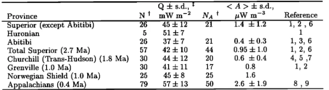
Table I summarizes the extensive data set now avail-

able for the Archeau and Proterozoic provinces of the Canadian Shield. The disposition of these provinces is

shown on the map (Figure 1). The average Archeau

heat flow, based on a total of 57 individual determi-

nations,

is 42 J: 10 mW m -2, 4 mW m -2 less than

estimated by $clater et al. [1980] and by Morgan and

$ass [1984]. In a world-wide

compilation

which does

Nyblade and Pollack [1993] found almost identical val- ues for the average and standard deviation of heat flow

values

in Archeau

regions

(41 J: 11 mW m-2). The

Trans-Hudson Orogen (formely Churchill Province) has

an average

heat flow of 44 mW m -2, slightly

higher

compatible with the idea that continental heat flow de- creases with age, but it is in fact due to the high heat

production in the Thompson Belt [Guillou-Frottier et al., 1996]. The absence of an age-dependent pattern is

confirmed by the Late Proterozoic Grenville province,

where the average heat flow is the same as that of

the Archeau. Heat flow is markedly higher in the Ap-

palachians, but this is again due to higher crustal heat

production

(Table 1). Jaupart

et al. [1982]

have

shown

erage heat flow in the Appalachians is identical to the average values in the Grenville and Superior. Indeed, in

their original

study,

Roy et al. [1968]

grouped

Grenville

a single heat flow province, because they all satisfied

the same heat flow versus heat production relationship.

The high Appalachian heat flow is due to a relatively

thin enriched upper crustal layer and provides no evi-

dence for mantle heat flow higher than in the Canadian Shield.

2.2. Bulk Crustal Composition in Precambrian

Shields

In this section, we compare estimates of the average

crustal heat production derived from various geochem-

ical and petrological models (Table 2). One approach

is to use average values for a set of representative rock

types and estimates

of their proportions

in a crustal

column

[Haack,

1983; Condie,

1993; Wedepohl,

1991].

A second approach relies on local exposures of terrains of various metamorphic grades, xenoliths suites and a

suitable

crustal

model [Rudnick

and Fountain,

1995].

A third approach is to follow a specific genetic model

for continental crust formation, for example, in island

arcs or in oceanic plateaus. The difficulty lies in assess- ing the reliability of the crustal model for comparison

with heat flow data. The continental crust is a highly

heterogeneous

mixture of old and young

crustal

rocks

intruded by mafic melts, and hence no simple petro-

logical logic can be followed. The recently

recognized

importance of mafic intrusions in the continental crust explains why simple petrological models, such as that by Wedepohl [1991], for example, invariably lead to the largest values of crustal radioactivity.

Table 1. Heat Flow Statistics for the Canadian Shield

Q •: s.d., • < A > •: s.d.,

Province N I mW m- •' NA I /•W m-3 Reference Superior (except Abitibi) 26 45 + 12 21 1.4 + 1.2 1, 2 , 6

Huronian 5 51 + 7 1

Abitibi 26 37 + 7 21 0.4 ß 0.3 1, 3, 6

Total Superior (2.7 Ma) 57 42 + 10 44 0.95 + 1.0 1, 2, 6 Churchill (Trans-Hudson) (1.8 Ma) 30 44 + 12 20 0.6 + 0.4 4, 5 ,7 Grenville (1.0 Ma) 30 41 :t: 11 17 0.8 1, 2 Norwegian Shield (1.0 Ma) 25 45 + 8 25 1.6

Appalachians (0.4 Ma) 79 57 :t: 13 50 2.6 :t: 1.9 8 , 9 References: 1, Pinet et al. [1991, and references therein]; 2, Guillou-Frottier et a/.,[1995, and references therein]; 3, Guillou et al. [1994]; 4, Drury [1987]; 5, Guillou-Frottier et al.

[1996]; 6, Mareschal et al., submitted manuscript; 7, Mareschal et al. [1997]; 8, Birch et al.

t Number of determinations.

15,272 JAUPART ET AL.' HEAT FLOW AND LITHOSPHERE THICKNESS

Hearne

$uperio

Province

Figure 1. Map showing the Precambrian in North America with the main provinces of the

Canadian Shield. K is the Kapuskasing structural zone. (Adapted from Hoffman [1989].)

Rudnick and Fountain [1995] have recently given a

comprehensive compilation of chemical analyses of lower crustal material. Unlike major elements and most trace

elements, Uranium and Thorium concentrations exhibit

highly skewed distributions. This may be attributed to their highly incompatible characteristics and, in the case of Uranium, to its large mobility. The median val-

ues of the distributions are systematically smaller than

the mean values. Rudnick and Fountain [1995, p.293]

chose to focus on the former values, in order to "mini- mize the effects of outliers in small sample populations." Another method is to assume that, in a province, con-

centrations for a given rock type are valid for all the province. Using geological maps, one may determine

the areas for each rock type and calculate an area- weighted average. In this case, the "outliers" are rock types which represent a negligible fraction of the crustal

assemblage. Using the studies of Ashwal et al. [1987], Fountain et al. [1987], as well as many other pub- lished reports, Pinet and Jaupart [1987] and Pinet et al. [1991] applied this method to four well-sampled differ- ent granulite facies terrains (the Kapuskasing and Pik-

witonei areas of the Superior Province, the Egersund

area in southern Norway, and the Ivrea Zone, Italy)

and three different amphibolite facies terrains from the Superior Province. For the granulites they found aver- age heat production values tightly clustered around 0.40

/•W m -3. Average values for three Australian granulite

Table 2. Crustal Models for Radiogenic Elements

U, Th, K20,

ppm ppm

•

/•W m- 3 Reference

Bulk crustal models

Andesite (whole Earth) 1.3 4.8 1.3 Andesire (Archeart) 1.8 3.3 0.9 Global crust/mantle budget 1.2 5.8 1.6 1.1 4.5 1.5

0.79 1 0.78 2 0.86 3 0.74 4

Archean upper crust

Shales 1.5 5.7 1.8 0.95 1

Direct sampling 1.2 9.6 2.4 1.20 5-7

References: 1, Taylor and McLennan [1985]; 2, Condie [1993]; 3, Allegre et al. [1988]; 4, Galer et al. [1989]; 5, Eade and Fahrig [1971]; 6, Ashwal et al. [1987]; 7, Fountain et al. [1987].

JAUPART ET AL' HEAT FLOW AND LITHOSPHERE THICKNESS 15,273

facies terrains with less data coverage are between 0.2

and 0.4/•W m -3. For the amphibolite facie•s terrains,

average heat production values are between 1.0 and 1.2

/•W m -3. These different

data sets are consistent.

We

shall use these values because they come from regions directly relevant to our heat flow data. For example, the Egersund region of the Norwegian Shield, which was once part of a continental block including the Grenville Province, provides a window into the Grenville lower

crust.

One useful reference is provided by a global chemical budget for the planet. The continental crust has been formed at the expense of the mantle. Thus one may de-

termine average crust and mantle compositions which are mutually consistent with one another and with the

bulk Earth composition [O'Nions et al., 1979; Galer et al., 1989; All•gre et al., 1983, 1988]. These various stud- ies lead to a small range of 0.74-0.86/•W m -a for the average heat production for all crustal ages, including rocks younger than Precambrian (Table 2).

The validity of crustal models may be assessed by

considering estimates for the upper and lower crust and

seismological constraints on crustal structure. The up- per crust may be sampled directly, and straight aver- ages have been made over large areas, most notably in the Canadian Shield [Eade and Fahrig, 1971; Shaw et al., 1986]. Others have taken shales as natural aver-

ages

of the upper crust [Taylor and McLennan,

1985].

These lead to values between 0.95 and 1.20 /•W m -a

ibr the upper crust, that is, those parts of the crust with metamorphic grade lower than granulite. For the lower crust we take the average heat production of gran-

ulite facies terranes,

0.40 /•W m -a. Using these esti-

mates, we may calculate a bulk crustal average given the proportions of upper and lower crustal material. In

the seismic shield models of Holbrook et al. [1992] and Durrheim and Mooney [1991], the lower crust is iden-

tified by higher seismic P wave velocities in the range

of 6.8-7.2 km s -•, and makes up 16 out of 45 km of

the crustal column. Taking values between 0.95 and

1.20/•W m -a for the upper crust and 0.40/•W m -a for

the lower crust, we find bulk Archean crustal averages

of 0.76 and 0.91 /•W m -a, respectively.

These values

are remarkably similar to those deduced from global chemical budgets. Average Archean crust is likely to

be poorer in radioelements than younger crust [Rud-

nick and Fountain, 1995]. Thus, for compatibility with

the global chemical budgets, we are led to select the

lower value of 0.76/•W m -a for the average

heat pro-

duction of Archean crust. Over a crustal thickness of

45 km, this implies a crustal heat flow component of 34

mW m -2. With the average

Archean

heat flow value

of 41 mW m -2, this leads to a mantle heat flow of 7 m•V m -2 .

The problem with such global reasoning is illustrated by the Canadian Shield, where the average crustal thick-

ness is 42 km. Rudnick and Fountain [1995] suggested

that the heat production in the Precambrian crust could be divided into Archean and Proterozoic, with an aver-

age heat production

of 0.51/•W m -3 and 0.89/•W m -3

respectively. These values would then yield mantle heat

flow values of 21, 7, and 4 mW.m -2, for the Superior,

Churchill, and Grenville provinces, respectively. Aver- age heat flow values vary within provinces because of changes in crustal structure and thickness. For exam- ple, the average heat flow in the Abitibi subprovince (37

mW m -2) is significantly lower than the average for the

Superior. This is due to the large amounts of greenstone

terranes with low radioactivity which are unaccounted

for in most global crustal models. Differences in heat flow and crustal structure between the Norwegian and the Canadian Grenville, that will be discussed later, are

another example of this problem.

Averaging over the whole Precambrian allows more

reliable comparisons between different data sets because

a major fraction of the continental crust is sampled and local heterogeneities are smoothed out. Furthermore, because of its large volume, the average Precambrian crust must be close to the bulk crust of the global chem- ical budgets. The average Precambrian heat produc-

tion is 0.84/•W m -a according to lrludnick and Foun- tain [1995], which is indeed within the range of the bulk

chemical

estimates

of 0.74-0.86/•W m -a. Following

Ny-

blade and Pollack [1993], the average heat flow through

Precambrian

continents

is 46 mW m -2, with a negli-

gible error of +1 mW m -2 due to uncertainties

in the

proportions of Archean and Proterozoic crust (see the

discussion by Rudnick and Fountain [1995]). For an

average Precambrian crustal thickness of 45 kin, the global estimates of crustal heat production lead to val-

ues of the mantle heat flow between 9 and 15 mW m -2.

Available estimates of bulk crustal heat production are in close agreement for Proterozoic provinces, in con- trast to Archean provinces for which there are large dis-

crepancies. For the Canadian Shield, the heat flow data

do not support the differences between Archean and Proterozoic crust suggested by some geochemical mod-

els. Because the mantle heat flow is a small residual

value, it is sensitive to even small errors on the crustal

heat production estimates. To ascertain our estimates,

we have looked in greater detail at the relationship be-

tween heat flow and local crustal structure.

2.3. Heat Flow in the Eastern Canadian Shield

A systematic study of the Canadian Shield has led to a detailed heat flow map of the Archean Abitibi sub- province and its boundaries with the Kapuskasing struc-

tural zone and the younger Grenville province [Pinet

et al., 1991; Guillou et al., 1994: Guillou-Frottier et

al., 1995]. Heat flow increases systematically from the

Grenville front to the Kapuskasing uplift over a dis- tance of m 500 kin. There is also a sharp drop of

about 20 mW m -2 over a distance of 70 km across the Ivanhoe Lake fault, which separates the Abitibi from

15,274 JAUPART ET AL' HEAT FLOW AND LITHOSPHERE THICKNESS

the Kapuskasing uplift. This demonstrates that these 500

variations of heat flow are of crustal origin (Figure 2).

The long-wavelength variation in heat flow is accom-

panied by an increase in Bouguer gravity. Taken to-

(/) 4oo-

gether

with seismic

results,

these

two data sets

provide

constraints that restrict crustal models and the man- .O_

tie heat flow to a very narrow range. In the Abitibi

'• 300-

subprovince,

three

crustal

lithologies

dominate:

green-

stones, tonalite-trondjemite-granodiorite, and granulite

facies

rocks. Large outcrops

of these

three lithologies

are exposed in the shield, allowing direct measurements

of their densities

and heat production

rates. •uillou et

al. [1994]

generated

a series

of

crustal

models

by

vary-

ing the mantle

heat

flow,

the thicknesses

of the three • 100

lithological units, their densities, and heat production rates. Only a limited number of models meet the con- straints of both gravity and heat flow data within the

error limits set at 2 mW m -2 for the heat flow and 0

4 mGal for gravity. These successful models represent

the whole set of solutions. The results can be illus- trated by a histogram of mantle heat flow values for the

models that fit the data within the given error limits

(Figure 3). Models could be found to satisfy the data

-20 • -30 - -40 - -50-

-60

longitude

Heat flow and gravity profiles across the

Figure 2.

Abitibi greenstone belt. The gravity profile is along

49øN; the heat flow profile includes all values between

48 øand 50 øN.

! i i

0 5 10 15 2o

Heat Flow mW m -2

Figure 3. Histogram of mantle heat flow values that yield a model compatible with gravity and heat flow data. The model assumes three crustal layers: green- stone metasedimentary and volcanics, tonalires, and lower crustal granulites.

only when the mantle heat flow lies between 7 and 15

mW m -2. The average and most probable values are

12 and 13 mW m -2, respectively. The value for the

Abitibi is within the range of the global Precambrian

models.

This result has been derived from a self-consistency argument over a large data set. Values of heat pro- duction for the upper and lower crust were not fixed but were left to vary. Thus, for example, fixing the heat production value of lower crustal assemblages at a

small value of 0.2 /•W m -3, say, requires

changing

all

the other variables.

2.4. Low Heat Flow Regions of the Canadian

Shield

The validity of the mantle heat flow estimate may be assessed by considering specific situations. In the Kapuskasing area, a reliable surface heat flow of 33

mW m -2 was •neasured in a deep borehole. In the area,

granulite facies terranes have been brought to the sur-

face by large thrust faults with low dip angles [Percival,

1994]. Measurements on rock samples from the gran-

ulite facies terranes in this area yielded an average heat

production

rate of 0.40 pW m -3 [Ashwal

et al., 1987].

Rocks from the borehole used for heat flow determina-

tion at Kapuskasing have an average heat production

rate of 0.46 pW m -s. A lower bound for the crustal

heat production is obtained by assuming that the en- tire crust has the same heat production than the gran- ulites. The crustal thickness in the Kapuskasing area is

JAUPART ET AL.' HEAT FLOW AND LITHOSPHERE THICKNESS 15,275

at least 45 km [Boland and Ellis, 1989; Percival et al., 1989; Wu and Mereu, 1992]. This yields a lower bound

of 18 mW m -'• for crustal

heat production

and conse-

quently an upper bound of 15 mW m -2 for the mantle

heat flow.

One might argue that low heat flow values are anoma-

lous and cannot be interpreted using an average lower

crustal composition. This is not consistent with the

observations:

low heat flow regions

(< 32 mW m -2)

are found throughout the Canadian Shield and corre- spond to large areas where the mid and lower crusts are exposed. For instance, very low heat flow values have been reported for the Adirondacks or in the lower

St. Lawrence valley, more than 500 km away from the

Grenville Front [Birch et al., 1968; Guillou-Frottier et al., 1995]. The heat flow profile across the Abitibi sub- province (Figure 2) shows that the heat flow values are

consistently

low in the east (27-28 mW m-•). The ab-

sence of dispersion gives confidence that the error on

these values is small. These values are found in a re-

gion that extends deeply into the Grenville Province

[Guillou

et al., 1994, Guillou-Frottier

et al., 1995]

and

is wider than several crustal thicknesses. Heat produc- tion rates cannot be uniformly low throughout the large

crustal volume sampled. For the estimated 40 km thick

crust, we calculate a lower bound of 16 mW m -• for crustal heat production and a mantle heat flow value of

12 mW m -•.

These simple calculations depend on the average heat

production of lower crustal material. In the Pikwitonei

and Kapuskasing areas, the deepest crustal levels have

not been sampled and one could argue that large pro-

portions of mafic rocks poor in radioelements lie in the deep crust. In the Ivrea Zone, Italy, where a crustal cross section extending down to the Moho is ex- posed, the average heat production of the lower crustal

rocks

is 0.40 •uW m -s [Galson,

19831. In the south-

30-32 mW m -• are found in and around the large

Sept-Iles gabbroic/anorthositic massif [Guillou-Frottier et al., 1995]. These exposures correspond to the same

structural crustal levels as in the Egersund-Bamble ar- eas of the Southern Norwegian Shield and are made of the same rock types. The extensive Norwegian data set

leads to a reliable estimate of 0.40/•W m -s for heat pro- duction in the granulite-facies crust [Pinet and Jaupart,

19871 . The crust below these two areas must be made

of the same granulite-facies material because there are no thrust faults. The Egersund heat flow value is 21

mW m -•' [Swanberg

et al., 1974].

For comparison

with

The heat flow difference of • 6 mW m -• is associated

with • 14 km difference in crustal thickness between

Southern

Norway [Pinet and Jaupart, 1987] and the

Sept-Iles area. This implies an average heat produc-

tion of about 0.43/•W m -s, not significantly

different

from our estimate of 0.40 •W m -s, as the errors on heat

flow and crustal thickness are about 4- 2 mW m -2 and

4-2 km, respectively. In the Egersund, the presence of large amounts of mafic rocks in the deep crust is ruled

out by gravity data [Smithson and Ramberg, 1979].

3. Mantle Heat Flow and Lithosphere

3.1. Small-Scale Convection Beneath the

Lithosphere

In a study of the thermal and dynamical stability

of continents, Doin et al. [1997] have considered the

supply of heat to the base of the lithosphere to bal- ance the conductive heat flow and the long-time sur- vival of a thick lithosphere in an actively convecting system. They have shown that it is necessary to in-

voke both a compositional density contrast and a vis-

cosity contrast between the lithosphere and the con- vecting mantle. Both types of contrasts are produced simultaneously by basalt extraction. The dehydration

of the solid residue increases its viscosity [Pollack, 1986; Hirth and Kohlstedt, 1996]. Partial melting depletes the

mantle in incompatible elements, implying low residual

uranium and thorium concentrations and hence small

radiogenic heat production. Support for the existence of a compositional density contrast comes from the study

of geoid anomalies [Turcotte and McAdoo, 1979; Doin

et al., 1996].

In eastern Canada the observations do not indicate

significant variations of the mantle heat flow beneath lithospheres of various ages, from the Arcbean to the

late Proterozoic. This shows that a stable thermal

regime has been reached in old continental lithosphere,

which requires a supply of heat at depth (Figure 4).

One may entertain three types of physical mechanisms for providing heat to the base of the lithosphere. The lithosphere may first be thought of as a passive body which is rafted on top of oceanic mantle and exchanges heat with it. This model is not compatible with a sec- ond class of models which are designed to investigate

O Tm Temperature

Conductive

boundary layer

Small-scale

convection

Figure 4. The model lithosphere showing the conduc- tive part and the unstable boundary layer beneath.

15,276 JAUPART ET AL.' HEAT FLOW AND LITHOSPHERE THICKNESS

the dynamical consequences of thick, and therefore in-

sulating, continental lithosphere. It may be shown that the continents generate large-scale thermal anomalies

in the mantle, which in turn induce convective currents whose dimensions depend on the width of continents

[Gumis, 1988; Zhong and Gurnis, 1993; Lenafdic and Kaula, 1996; Guillou and Jaupart, 1995]. In these two

types of models, the continental lithosphere has spec- ified characteristics, that is, thickness, rheology, and density, and the problem of what determines them is not addressed. A di•culty is that it is not possible to study the continental problem independently of con- vection through the whole mantle. A third mechanism

to provide heat is small-scale convection, which can be

studied extensively and locally. We determine the con- ditions for small-scale convection to supply the required heat flux at the base of the continental lithosphere and

we calculate the thickness of the lithosphere and the

temperature of the underlying mantle. We also discuss transient conditions over geological time scales.

3.2. Small-Scale Convection in Variable

Viscosity Liquids

The Earth's mantle is cooled from the top and has a

large temperature difference across its upper boundary layer. This temperature difference implies large viscos- ity variations. In such conditions, the upper part of the boundary layer is not involved in convective instabili-

ties and remains stagnant [Richter et al., 1983; Fleitout

and Yuen, 1984; Buck and Parmentier, 1986; White,

1988; Ogawa et al., 1991; Davaille and Jaupart, 1993a].

Convection is confined to a relatively thin layer where viscosity variations are small, and its characteristics de-

pend on the viscosity function [Jaupart and Parsons,

1985]. Small-scale convection is a feature of many con- vection models (see the discussion by Davaille and Jau- part [1994]) and may coexist with large-scale convective currents with little modification [Parsons and McKen- zie, 1978; Doin et al., 1997].

A recent laboratory study at large viscosity contrasts

[Davaille and Jaupart, 1993a] has shown that convec-

tion depends solely on variables defined locally in the unstable boundary layer. For a given interior temper- ature Tin, the convective heat flux Q does not depend on the surface temperature and is given by

Q - 0.47kin(

ag )x/3ATv4/3

(1)

•ly m

where g is the acceleration of gravity, kin, a, •, and Ym are thermal conductivity, coefficient of thermal ex- pansion, thermal diffusivity, and kinematic viscosity, re- spectively. ATv is the convective temperature scale de-

fined as

.(Zm) XTv = -

(d/•/dT)(Tm)

where /• is viscosity. This equation was derived from scaling arguments and laboratory measurements of con-

vection. The laboratory experiments were made for dif- ferent rates of viscosity variations as a function of tem- perature and for different viscosity contrasts. Davaille

and Jaupart [1993b] have succesfully applied their re-

sults to lava lakes, where the effects of convection can be

recorded directly. This indicates that the scaling laws are applicable to a wide range of variable viscosity ma- terials. The same scaling laws were obtained by numer- ical calculations over a large range of Rayleigh numbers

and viscosity contrasts (O. Grasset, personal communi-

cation, 1997; C.$otin, personal communication, 1997]

and with non-Newtonian fluids with temperature and

pressure dependent viscosity [Doin et al., 1997]. In this

case, one must take the viscosity parameters at the top of the unstable boundary layer, that is, at the base of

the stagnant and conducting lid (Figure 4).

Scalings have also been obtained for the temperature difference across the convective boundary layer AT and

the thickness of this boundary layer 5 [Davaille and Jau- part, 1993a]:

AT • 2.2ATv

5 • 6.2 AT

(3)

agAT)

-x/3 (4)

where AT,• - T,• -To is the temperature difference

across the stagnant and conductive lid (i.e., the litho-

sphere). These parameters allow us to calculate the

temperature in the well-mixed mantle below the con- vective boundary layer.

3.3. The Heat Flux Supplied to the Base of the

Lithosphere

These results can be applied to the continental litho-

sphere once the rheology of the upper mantle rocks is

specified. Kavato and Wu [1993] have summarized cur-

rent knowledge based on laboratory measurements, the solid-state physics of deformation in minerals at high temperature as well as constraints from postglacial re- bound studies. The strain rate/stress relation takes the general form:

• -(• + •V)

• -- A(

cr

)n(•)

TM

exp(

)

(5)

size, and E and V are the activation energy and vol-

ume, respectively. Following Karato and Wu [19931, we take • - 8 x 10 •ø Pa, b- 5 x 10 -lø m, and d- 1 min. Values for coefficient A are also taken from their

paper. The exponents n and m depend on the creep mechanism. For dry and wet dislocation creep, n • 3.5 and • 3.0, respectively, and m - 0; for diffusion creep, n • I and m • 3. The effective viscosity • is deter- mined by

JAUPART ET AL- HEAT FLOW AND LITHOSPHERE THICKNESS 15,277

where a0 is the second-order stress invariant. Introduc-

ing the values of the parameters in (6), we obtain the

final relationship'

E+PV

/• - C exp

( RT )

(7)

where C is a constant for diffusion creep; and C de- pends on the stress level for dislocation creep. In the present paper, we chose a value of 1 MPa for the stress level due to small-scale convection. However, it will be seen that dislocation creep cannot account for the observed mantle heat flow regardless of the reference stress level chosen. Table 3 gives the parameter val- ues relevant to the upper mantle for four deforma- tion mechanisms- dislocation creep in dry and water-

saturated ("wet") olivine, diffusion creep in dry and water-saturated ("wet") olivine. According to Karato

and Wu [1993], the most likely deformation mechanism

deeper than • 200 km is diffusion creep in rocks con- taining some water without being saturated. For the subcontinental mantle, therefore, one expects a linear rheology with parameters between those for dry and

wet olivine.

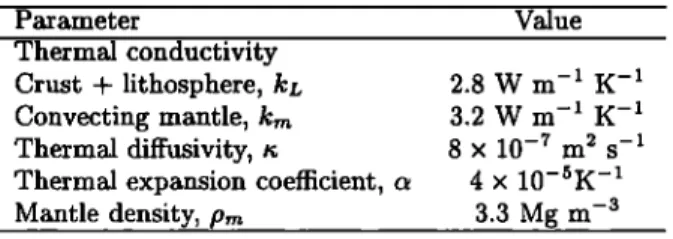
To evaluate these results in the context of the heat

flow constraints, we first fix the base of the lithosphere at a depth of 250 km. We use values for the relevant physical properties listed in Table 4. Thermal conduc- tivity depends mostly on temperature for the pressure range of this problem and includes the effects of both

phonons and photons. Below the lithosphere, tempera-

tures are larger than 1550 K, and available laboratory measurements indicate a value of thermal conductivity

• 3.2 W m -• K -x [Schatz

and Simmons,

1972;

Roy et

al., 1981; $chSrmeli, 1979]. We return to this question

later, but we note that because the convective heat flux

depends

on k •'/3, it is not very sensitive

to the specific

value chosen. For a given viscosity law, temperature is

the only unknown. Using (1) for the small-scale convec-

tion heat flux, we calculate heat flow as a function of

temperature (Figure 5). For the purposes of discussion,

we consider

a range of 10-14 mW m -•' for the man-

tle heat flow. For these values, dry-dislocation creep requires temperatures in excess of 2050 K. The other

creep mechanisms require temperatures between 1550

and 1900 K. In the well-mixed oceanic upper mantle,

Table 3. Parameters for Mantle Viscosity Laws

C, E, V,

Creep Mechanism Pa s kJ mol- x cmS.mol - x Dry diffusion 5.19 x 10 xø 300 6

Wet diffusion 8.55 x 10 TM 240 5

Dry dislocation 4.14 540 20

Wet dislocation 2.56 x 10 •' 430 15

The parameters for dislocation creep have been calculated

for a reference stress level of I MPa.

Table 4. Physical Properties of Lithosphere and

Upper Mantle Parameter Value Thermal conductivity Crust -!- lithosphere, k L Convecting mantle, k,• Thermal diffusivity, n

Thermal expansion coetficient, Mantle density, p,• 2.8 W m -x K -x 3.2 W m -1 K -x 8 x 10 -7 m •' S --1 4 x 10-SK -x 3.3 Mg m -s

away from upwellings and subduction zones, the ref- erence isentropic decompression path corresponds to a

potential temperature of about 1550 K [McKenzie and

Bickle, 1988]. At 250 km, this predicts a temperature of

about 1700 K. The uncertainty on this estimate is prob- ably • 50 K. Seismic tomography results do not indi-

cate that the mantle is hotter beneath continents than oceans [Anderson, 1990]. Thus these considerations rule

out dry diffusion creep as a rheology compatible with

the heat flux and the mantle temperature. Wet diffu-

sion creep, or a rheology intermediate between dry and

wet diffusion creep in olivine, meets the constraints. We also calculate viscosity values at the same refer-

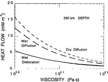
ence depth of 250 km (Figure 6). Postglacial rebound

studies yield an average viscosity for the upper man-

tle beneath the lithosphere which is between 1021 and

5 x 10

•'x Pa s, according

to various

authors

[McConnell,

1968; Peltier, 1981; Nakada, 1983]. For diffusion creep,

viscosity increases with depth through the upper man- tle along an isentropic temperature profile by a factor of about 20. For dislocation creep, this increase is several orders of magnitude larger. Thus the average upper mantle viscosity values imply that the local viscosity at the base of the lithosphere should lie between about

102ø and 5 x 10 •'ø Pa s for diffusion creep and should be less than 10 •s Pa s for dislocation creep. Figure 6 shows

that mantle heat flow values for diffusion creep are com- patible with the postglacial rebound constraints.

The above results are modified only slightly if other values for the physical properties are selected within their probable ranges. The activation volume has a negligible effect on the results if it is varied between

the bounds quoted by Karato and Wu [1993].

In conclusion, the mantle heat flow values derived

in section 2 may be supplied to the base of the conti- nental lithosphere if the deformation mechanism of the upper mantle is diffusion creep. The predictions for wet diffusion creep are in agreement with all available constraints, that is, viscosity values from postglacial re- bound studies, the likely range of continental mantle

temperatures.

3.4. Thickness of the Lithosphere

In steady state conditions, the mantle heat flow is transported by conduction through the lithosphere.

15,278 JAUPART ET AL.: HEAT FLOW AND LITHOSPHERE THICKNESS

•,• 40

20

Figure 5. Mantle heat flow supplied by small-scale

convection as a function of mantle temperature at 250

km depth. Three different creep laws have been used, with parameters given in Tables 3 and 4.

Thus one may calculate the vertical temperature profile from the surface downwards using heat flow constraints. We may write the temperature in the mantle part of the lithosphere as follows:

o•z

Z

Q•

- Tc

+

where the mantle conductivity kœ depends on tempera- ture. Tc is the temperature at the Moho discontinuity, which depends on the surface heat flow Q s, on the dis- tribution of radiogenic heat production in the crust and on the values of conductivity of crustal rock types. De-

tailed calculations for specific cases [Pinet et al., 1991]

yield for Tc a value of 673 + 100 K. Throughout most of the following, we shall take a value of 673 K. We shall neglect heat generation in the mantle part of the lithosphere because it is likely to be very small.

The value of thermal conductivity kœ is critical. Ther- mal conductivity depends mostly on temperature for the pressure range of this problem and includes the ef- fects of both phonons and photons. Thermal conduc-

tivity has a typical average

value of 2.5 W m -1 K -• in

the continental crust [•'lauser and Huenges, 1995] and

is expected to increase in the mantle part of the litho- sphere. We have used the following equation for the mantle thermal conductivity as a function of tempera-

ture:

1

k•(T)- 0.174

+ 0.000265

T + 0.368

10

-9 T 3 (9)

where T is in kelvins [Doin and Fleitout, 1996]. This

equation is consistent with the available laboratory data

[Schatz and Simmons, 1972; SchSrmeli, 1979; Roy et

al., 1981] and gives an average conductivity value of

3.0 W m -1 K -1 in the 273-1600

K temperature

range.

It may be emphasized that, because of (8) for temper-

ature, the average conductivity value does not lead to the average geotherm. The uncertainty on thermal con- ductivity is difficult to assess. The difficulty of mak- ing measurements at high temperatures implies a small

data set [Schatz and Simmons, 1972]. Other sources of uncertainty are due to anisotropy [SchSrmeli, 1979] and to the fact that measurements are made on individual

minerals, which makes the evaluation of the bulk prop- erty of the polycrystalline mantle assemblage difficult. It is therefore useful to make direct large-scale estimates on the oceanic lithosphere. This may be achieved using the systematics of heat flow, depth and geoid anoma-

lies in young ocean basins [Lister, 1982; Gibert and Courtillot, 1990; Doucourd and Patfiat, 1992] and leads

to bulk conductivity values in the range of 2.7 - 2.9

W m -1 K -1. These are significantly lower than fre-

quently assumed values, as already emphasized by Lis-

ter [1982], and are compatible with the predictions of (9). We found that differences are negligible between calculations with a conductivity given by (9) and with a constant conductivity value of 2.8 W m -1 K -1. From

this discussion we estimate that the uncertainty on con-

ductivity at high temperature is less than 20%.

With these values, we may calculate a geotherm for

a given value of mantle heat flow. We shall require that

the same heat flow is supplied by small-scale convection

beneath the lithosphere, using (1) and viscosity function (7), which provides a second relationship between tem- perature and depth. The two temperature versus depth curves intersect at a given temperature and depth (Fig- ure 7). This defines the stable solution, that is, such

that the conductive heat flux across the lithosphere is

supplied by small-scale convection underneath it. The characteristics of small-scale convection are evaluated

20 E 15 E v I-- <I: 5 Wet % Diffusion • Dislocation o 1 020 250 km DEPTH "'- Dry Diffusion 1 021 1 022 VISCOSITY (Pa s)

Figure 6. Mantle viscosity as a function of mantle

heat flow for a depth of 250 km for the same cases as Figure 5.

JAUPART ET AL' HEAT FLOW AND LITHOSPHERE THICKNESS 15,279 0 lOO I 2OO 300 400 TEMPERATURE (K) 1000 2OOO

'',

/ Qm=

12mWm'2

j

400

300

200

lOO lO

Constant thermal conductivity

•

in

lithosphere

(2.8

W

m"K")

•

• .•Dryjfusion

_

_ Wet

diffusion•

15

20

HEAT FLOW (mW

m

'2)

tive lithosphere

for a mantle heat flow of 12 mW m -2.

Also shown is the relationship between depth and tem- perature which is required for small-scale convection to supply the same heat flux. ILl

z

for the values of temperature and pressure at the base of the conduction region. Thus one must add the unsta- m ble boundary layer in order to reach the fully convecting m

mantle (Figure 4). For our purposes it is more useful to

use the purely conductive upper layer because it is this O

layer

which

survives

over

large

time scales.

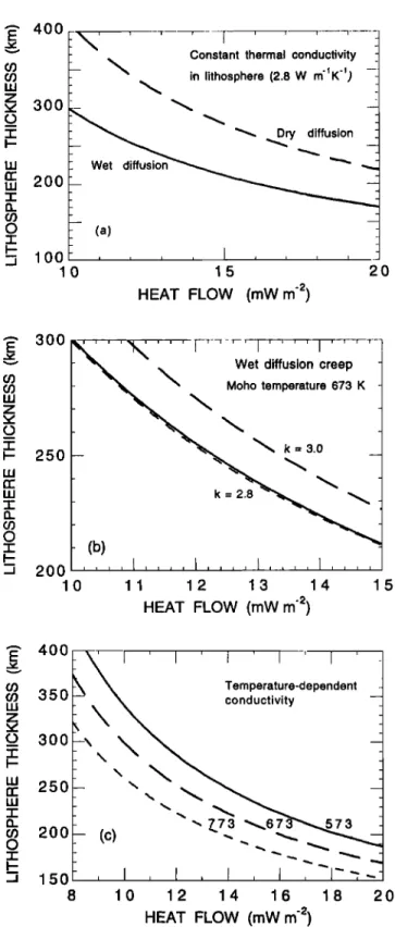
-r

creep. For a mantle heat flow value fixed at 13 mW m -2 (see above), we find a range of 240-320 km due to the uncertainty on the water content of mantle minerals. A

recent

study [Hirth and Kohlstedt,

1996]

suggests

that

the water

contents

of mantle

minerals

are sufficient

to

values. In this case, the "wet" values adopted in this

paper would be closest to reality. The numerical re- sults are sensitive neither to the values of thermal con-

ductivity adopted (Figure 8b) nor to the specific Moho rr

temperature

selected

(Figure

8c) Changing

the Moho m

temperature

by 100

K changes

the lithosphere

thickness

by less than 25 km. The effect of increasing the Moho O

temperature, for example, is compensated by the larger

values

of mantle

conductivity.

The range of lithospheric thicknesses could be nar- rowed down by adding constraints from other geophys- ical studies, but this is outside the scope of this paper. For a given creep law, the lithosphere thickness is sen-

sitive to the mantle heat flow value (Figure 8a). In

contrast, the basal temperature does not change much when the mantle heat flow is varied within its probable

range (Figure 9). The reason for this behavior is that

viscosity is very sensitive to temperature and much less so to pressure because of the relatively small value of

the activation volume. For example, for wet diffusion

creep, the basal temperature is constrained to lie be-

tween 1615 K and 1635 K for mantle heat flow values

300

250

20O

10

'•

•

Wet

diffusion

creep -

•• •høtemperature673K

I

_

"•,-• • k=3.O

(b)

HEAT

FLOW

(mW

m

'2)

-

"-2'.-_'"'---_

HEAT

FLOW

(row

m

'•)

Figure 8. (a) Lithosphere thickness as a function of

mantle heat flow for diffusion creep. The Moho tem-

perature is taken to be 673 K. (b) Lithosphere thick- ness as a function of mantle heat flow for "wet" diffu-

sion creep law. The thermal conductivity of the litho-

sphere

is taken to be 2.8 W m -1 K -1 (solid curve),

3.0

W m -1 K -1 (long dashes),

and fully temperature

de-

pendent (small dashes). (c) Lithosphere thickness as

a function of mantle heat flow for wet diffusion creep

and for three different Moho temperatures (in kelvins).

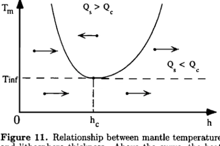
Thermal conductivity varies with temperature in the