Design and construction of an apparatus for induction heating for controlling DNA hybridization

_ II

MITLibraries

Document Services

http://libraries. mit. edu/docs

DISCLAIMER OF QUALITY

Due to the condition of the

original material, there are unavoidable

flaws in this reproduction. We have made every effort possible to

provide you with the best copy available. If you are dissatisfied with

this product and find it unusable, please contact Document Services as

soon as possible.

Thank you.

Some pages in the original document contain

Design and Construction of an Apparatus for Induction Heating for Controlling DNA Hybridization

by

Maria E. Tanner

Submitted to the Department of Mechanical Engineering in Partial Fulfillment of the Requirements

for the Degree of

Bachelor of Science

at the

Massachusetts Institute of Technology

June 2004

©C) 2004 Maria Tanner All rights reserved

The author hereby grants to MIT permission to reproduce and to

distribute publicly paper and electronic copies of this thesis document in whole or in part.

Signature of Author ...

...

...

Department of Mechanical Engineering May 24, 2004

Certified

by ... , ...

Kimberly Hamad-Schifferli Assistant Professor of Mechanical Engineering

Thesis Supervisor

Accepted

by...

Ernest G. Cravalho Professor of Mechanical Engineering Chairman, Undergraduate Thesis Committee MASSACHUSE-FS INSTITUTE

OF TECHNOLOGY

OCT 2 8 2004

DESIGN AND CONSTRUCTION OF AN APPARTUS FOR

INDUCTION HEATING FOR CONTROLLING DNA HYBRIDIZATION

by

MARIA ELISA TANNER

Submitted to the Department of Mechanical Engineering on May 24, 2004, in partial fulfillment of the requirements for the Degree of Bachelor of Science in

Mechanical Engineering

ABSTRACT

The purpose of this investigation was to design and construct a coil that could be used to selectively heat nanoparticles attached to "molecular beacons" or DNA loop/hairpin structures. Testing was conducted to see if the heat would be sufficient to open the molecular beacon by dehybridizing the dsDNA. This was accomplished by developing a series of seven coils that were tested using a network analyzer and through scans

conducted on a fluorometer.

The initial design requirements for the coil were that it needed to heat the nanoparticle, should be suitable for optical testing, and require a relatively small sample volume. At the end of the design and testing period, however, a coil that met these requirements was not successfully constructed, but two additional design requirements were developed.

Through temperature testing, it was realized that the primary heating of the solution was occurring due to the coil being heated through the power. As a result, a coil that

eliminates this source of power dissipation needs to be developed through the use of an air gap, water bath, or similar application, which can draw some of the heat away from the solution. Secondly, in constructing the coils, each was wound tightly so that there was a minimal gap between each loop. However, experiments showed that the proximity effect on resistance could not be neglected. This provided information on future possible designs. Therefore, the coil should be wound so that there is at least one wire's width of gap between each loop.

Thesis Supervisor: Kimberly Hamad-Schifferli Title: Assistant Professor of Mechanical Engineering

Acknowledgements

I especially would like to thank my thesis advisor, Professor Kimberly Hamad-Schifferli for all of her help and guidance. I enjoyed being a part of her lab group and having the opportunity to work with her over the last year. Andy Wijaya has also been an invaluable resource to me. I greatly appreciate all the time and effort he spent to ensure that I understood the research and the goal of my experiment. Thank you also to Peggy Garlick for making sure I fulfilled all my requirements for graduation and for always having the door to her office open. Finally I would like to thank my family: Dad, Mom, Melissa, Melinda, Buck, and Margaret. You have always been there for me and I love you.

Table of Contents 1.0 Introduction 6 2.0 Theoretical Analysis 8 2.1 Magnetic Fields ... 8 2.2 Coil Theory ... 9 2.3 Helmholtz Coil ... 11 2.4 Molecular Beacon ... 12 2.5 Particle ... 13 2.6 Fluorometer ... 13 3.0 Experimental Procedure 15 3.1 Apparatus ... 15 3.1.1 Cuvette ... 15 3.1.2 Fluorometer ... 15 3.1.3 Network Analyzer ... 17 3.2 Methods ... 17 4.0 Results 19 4.1 Existing Coil ... 19 4.2 MT1: Helmholtz Coil ... 19 4.3 MT2 ... 22

4.4 MT4, MT5, MT6: A comparison in coil length. ...25

4.5 MT7 ... 32

4.6 Temperature Probe ... 35

4.7 Summary of Coils ... 37

Table of Figures

FIGURE 1: PERMANENT MAGNET DEPICTING THE MAGNETIC FIELD, MAGNETIC FIELD LINES,

AND THE MAGNETIC FIELD DENSITY ... 8

FIGURE 2: A CIRCULAR LOOP OF CURRENT AND THE RESULTING MAGNETIC FIELD ... 9

FIGURE 3: SOLENOID MAGNETIC FIELD ... 10

FIGURE 4: AN IDEALIZED SOLENOID IS SHOWN IN THE BOLD LINES WITH THE MAGNETIC FIELD LINES. THE RECTANGULAR AMPERIAN LOOP ABCD IS SHOWN WITH THE DASHED BOX ... 10

FIGURE 5: HELMHOLTZ COIL ... 11

FIGURE

6: FROM LEFT TO RIGHT, THE MOLECULAR BEACON IN ITS NONHYBRIDIZED STATE

FIGURE 7: MOLECULAR BEACON WITH MAGHEMITE PARTICLE ATTACHED; WHEN THE PARTICLE IS HEATED THE MOLECULAR BEACON OPENS AS SEEN ON THE RIGHT ... 13

FIGURE 8: PLOT SHOWING DATA FROM AN EXCITATION AND EMISSION SCAN OF RHODAMIN ... 14

FIGURE 9: SCHEMATIC DEMONSTRATING LIGHT ENTERING AND EXITING A CUVETTE ... 15

FIGURE 10: PICTURE DEPICTING THE BASIC PLATFORM AND ITS ORIENTATION FOR LIGHT EMISSION AND ABSORPTION WITHIN THE FLUOROMETER ... 16

FIGURE 11: ABS VERSION OF THE BASIC PLATFORM ... 17

FIGURE 12: EXISTING COIL ... 19

FIGURE 13: PICTURE OF MT 1 ... 20

FIGURE 14: GRAPHICAL NETWORK ANALYZER DATA FOR MT 1

...21

FIGURE 15: PICTURE OF MT2 ... 23

FIGURE 16: GRAPHICAL NETWORK ANALYZER DATA FOR MT2 ... 23

FIGURE 17: TIME SCAN PLOT FOR MT2 AT 1GHZ AND 1 MHZ ... 25

FIGURE 18: PICTURE OF MT4, MT5, MT6 ... 26

FIGURE 19: NETWORK ANALYZER DATA FOR MT4 ... 27

FIGURE 20: NETWORK ANALYZER DATA FOR MT5 ... 28

FIGURE 21: NETWORK ANALYZER DATA FOR MT6 ... 29

FIGURE 22: TIME SCAN OF MT4 AT 1 MHZ AND 1 GHZ ... 31

FIGURE 23: TIME SCAN OF MT5 AT 1 MHZ AND 1 GHZ ... 31

FIGURE 24: PICTURE OF MT7 ... 32

FIGURE 25: NETWORK ANALYZER DATA FOR MT7 ... 33

FIGURE 26: TIME SCAN PLOT FOR MT7 AT 1 GHZ AND 1 MHZ ... 34

FIGURE 27: (A) SETUP WITH THE TEMPERATURE PROBE PLACED IN THE SOLUTION AND (B) SETUP WITH THE TEMPERATURE PROBE PLACED ON THE COIL ... 35

1.0 Introduction

The Hamad-Schifferli Group at MIT is working on developing a way to "demonstrate remote electronic control over the hybridization behavior of DNA molecules, by

inductive coupling of a radio-frequency magnetic field to a metal nanocrystal covalently linked to the DNA" [1 ]. They are currently using molecular beacons with an iron oxide particle attached. When the particle is heated, the DNA molecular beacon changes conformation from a stem and loop to an open configuration. This can be measured through the use a fluorophore that linked to one of the beacon. When the particle is unheated, the DNA is in a closed conformation and the fluorophore does not fluoresce. However, when the particle is heated and the beacon opens, the fluorophore fluoresces which can be measured.

This research has a number of implications. The heating of the particle and resulting denaturation of the DNA is very localized. This research could be applied to a wide range of applications that require the control of biological molecules such as a

non-invasive and less harsh treatment for cancer or through biological robots.

There are several concepts within this area of research that are currently unknown. For example, little is understood about the heating mechanism of the particle. The heating of the iron oxide particle is achieved through the use of the magnetic field generated by a coil. An iron oxide particle has been chosen because they are known to heat in an alternating magnetic field. They are also easy to obtain and can be used in high volume fractions of approximately 10%.

Similarly, how to construct an apparatus to test for the heating of the particle is unknown. The purpose of this investigation was to design and construct a coil that could be used to selectively heat nanoparticles attached to molecular beacons or dsDNA, and to conduct testing to see if the heat would be sufficient to open the molecular beacon or dehybridize the dsDNA.

The primary design requirement for the coil is that it needs to be able to heat the iron oxide particle. It is also desirable for the coil to fit inside the fluorometer required for optical testing and that it should require a relatively small sample volume. Once a successful coil has been developed, the laboratory group will be able to use it to probe physical properties of biomolecules while being controlled by nanoparticle heating.

2.0 Theoretical Analysis

This section outlines some of the theoretical concepts and background used in developing the appropriate coil.

2.1 Magnetic Fields

The magnetic field, B, is "the space outside a magnet" [2]. It is created by a moving electric charge and exerts a force on any other moving electric charges or currents that are present in the field [3]. Figure 1 shows the magnetic field of a permanent magnet. The dotted lines are magnetic field lines; they represent the strength and direction of the magnetic field. The magnetic flux, , is "the entire group of magnetic field lines which can be considered to flow outward from the north pole of a magnet" [2]. While the magnetic field is a vector quantity, magnetic flux is a scalar quantity that equals

¢, = iB-dA,

(1)

where A is the area of the surface [3]. The magnetic flux density is "the number of magnetic field lines.. .per unit area in a section perpendicular to the direction of the flux"

[2].

7~~~~~

-_--"~~~- ... .- ''.. I~

1 cm square

Figure 1: Permanent magnet depicting the magnetic field, magnetic field lines, and the magnetic field density

(2)

B= t°i

2nzR

where [t, is the permeability constant and equals 4r x 10- 7_{Tm/A, i is the current through}

the long wire, and R is the radius [2, 3, 4, 5]. This equation demonstrates that the magnetic field decreases with increasing distance from the wire. "Bending a straight conductor in the form of a loop" results in "the magnetic field lines are [denser] inside the loop. The total number of lines is the same as the straight conductor, but in the loop, the lines are concentrated in a smaller space" [2]. Figure 2 demonstrates this effect.

B

Figure 2: A circular loop of current and the resulting magnetic field.

2.2 Coil Theory

A solenoid is a useful way of generating a uniform magnetic field. "A solenoid is a long wire wound in a close-packed helix and carrying a current i" [5]. Based on the

assumption that the solenoid is closely packed, each turn can be considered a planar circular loop. An ideal solenoid has a length that is much longer than its diameter. An illustration of the magnetic field of a solenoid is shown in Figure 3.

~,

;... ...

Figure 3: Solenoid magnetic field.

To find the magnetic field due to a solenoid, Ampere's Law is applied

B . ds=,uoi, (3)

where ds is an increment of length [3, 5].

d

c

(~~~~~~~~~~~~~

a

--

Figure 4: An idealized solenoid is shown in the bold lines with the magnetic field lines. The rectangular Amperian loop abed is shown with the dashed box.

Applying a rectangular path abcd to an ideal solenoid, see Figure 4, yields

b c d a

B. ds =

B

+B

+B

(4)

a b c d

which can be simplified to

B = oiOn (5)

which describes the magnetic field of a solenoid, where n is the number of turns per unit

2.3 Helmholtz Coil

A Helmholtz coil (Figure 5) is a special version of a coil that consists of "a parallel pair of identical circular coils spaced one radius apart and wound so that the current flows through both coils in the same direction" [4].

R

Figure 5: Helmholtz Coil

This arrangement results in "an extremely uniform low frequency magnetic field between and in the center of the coils" where "the strength of the magnetic field generated is directly proportional to the number of turns in the coils and the current applied to them" [4]. "The purpose of the arrangement is to obtain a magnetic field that is more nearly uniform than that of a single coil without the use of a long solenoid" [4].

For a circular Helmholtz coil, the magnetic field is can be calculated from:

NI

B = 0.715-,

R (4)

where N is the number of turns of turns per coil, I is the coil current, and R is the radius [4]. This equation can be used to determine the magnetic flux density using:

H =

,uaoB

8.99x 0-7/

,

R (5)

2.4 Molecular Beacon

Molecular beacons consist of a "single stranded oligonucleotide hybridization probes that form a stem-and-loop structure" with a fluorophore covalently linked to one end and a quencher covalently linked to the other end [6]. When molecular beacons are free in solution they do not fluoresce because "the stem places the flurophore so close to the nonfluorescent quencher that they transiently share electrons, eliminating the ability of

the fluorophore to fluoresce" [6]. However, "the loop contains a probe sequence that is complementary to a target sequence" and when molecular beacons "hybridize to a nucleic acid strand containing a target sequence they undergo a conformational change that enables them to fluoresce" since the quencher is no longer located as close to the fluorophore [6]. Figure 6 demonstrates both conformations of the molecular beacon.

Figure 6: From left to right, the molecular beacon in its nonhybridized state with the fluorophore and quencher close together eliminating the fluorophore's ability to fluoresce; with the molecular beacon encounters a target sequence and hybridizes it changes conformations which allows the fluorophore to fluoresce 16].

The molecular beacon used in these experiments is:

5' - GCG AGT TTT TTT TTT TTT TTC TCG C - 3'.

Molecular beacons are widely used because of their ability to differentiate target sequences down to a single nucleotide difference [6]. They are very specific and will only bind and maintain a stable conformation if the target sequence is the perfect

complement to the loop. Here they are used not to detect if a particular sequence of DNA is present, but rather as a temperature sensor. Increased temperature causes the molecular beacon to open, increasing the fluorescence.

2.5 Particle

A maghemite particle is attached to the molecular beacon, so that when the particle is heated the molecular beacon goes into the open conformation enabling the fluorophore to fluoresce, see Figure 7. The particle is an iron oxide particle (Fe304) purchased from Ferrotech as EMG-507. Fe304 F Q Fe304 I

F

Figure 7: Molecular beacon with maghemite particle attached; when the particle is heated the molecular beacon opens as seen on the right

In addition, the iron oxide particles can be mixed in solution with the molecular beacon.

2.6 Fluorometer

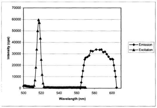
The Spex FluoroMax-3 is a highly sensitive spectrofluorometer, which "excites [the sample] with one color of light, then looks at the color that results when the light is re-emitted" [7]. Changes in color and intensities can be used to determine molecular size, atomic distances, or crystal structure.

The fluorometer has three primary scans that were used: emission scans, excitation scans, and time scans. Emission scans and excitation scans are used to verify the wavelength calibration of the sample. The excitation scan measures how much light is being absorbed by the solution while the emission scan measures how much light is being

.0

-emitted by the solution. Typical emission and excitation plots for the solution used in this experiment are shown in Figure 8.

70000 60000 50000 Cf 40000 a. D 30000 20000 10000 0 500 * Emission 1 A Excitation 520 540 560 580 600 Wavelength (nm)

Figure 8: Plot showing data from an excitation and emission scan of rhodamin

For the sample used in this experiment, the emission wavelength is 581.5nm, and the excitation wavelength is 556nm.

3.0 Experimental Procedure

This section overviews the experimental apparatus and methods used in testing each coil and ultimately, the heating of the particles.

3.1 Apparatus

The following sections describe the different components of the experimental apparatus.

3.1.1 Cuvette

A cuvette is a small vessel in which the solution is placed. Various cuvettes were obtained and used in this experiment including quartz cuvettes and plastic cuvettes. The most important requirement in selecting the cuvette used was that all four sides had to be transparent so that the light could enter and leave at a right angle (see Figure 9).

- OUT

IN

Figure 9: Schematic demonstrating light entering and exiting a cuvette

3.1.2 Fluorometer

The Spex FluoroMax-3 is a highly sensitive spectrofluorometer, which "excites [the sample] with one color of light, then looks at the color that results when the light is re-emitted" [7]. Changes in color and intensities can be used to determine molecular size, atomic distances, or crystal structure.

The lab uses three attachments to test coils and samples in the fluorometer. These are the basic platform, Fluoromax Peltier, and the Fiber Optics. Each attachment is used for a subsection of scenarios. For example, the basic platform is for small holders, such as cuvettes, that can be tested directly inside the fluorometer. The Fluoromax Peltier is used

for temperature-controlled situations, and the Fiber Optics option is used when the solution and holder are too large to be tested inside the fluorometer.

The basic platform is a hardened steel platform that screws inside the fluorometer, oriented so that the slits of the solution holder align with the light being emitted and collected (Figure 10).

Metal original part)

Figure 10: Picture depicting the basic platform and its orientation-for light emission and absorption within the fluorometer

Wrapping the coil directly around the ABS holder or around the cuvette eliminated the use of the larger coils and the need for the fiber optics attachment. Because the coil now can be located inside the fluorometer, greater care had to be taken in ensuring that the magnetic field was not being affected by the presence of metal. Therefore, a new ABS basic platform was designed and constructed, which is shown in Figure 11, to replace the original basic platform.

Metal (original part)

Figure 11: ABS version of the basic platform

While performing the scans, all openings to the fluorometer are sealed to prevent any light from entering and altering the emission and excitation data.

3.1.3 Network Analyzer

An Agilent 8753S S-parameter Network Analyzer is used to test the coils in a frequency range of 30kHz to 6GHz. At each frequency, the resistance can be determined using S 11 measurements in which power is sent through the coil and then the reflected power is measured.

3.2 Methods

For each coil, several tests were performed to ensure that the setup was working

correctly, that the coil was working, and to test whether the particle was being heated or not. In order to do this, three scans were used on the fluorometer: emissions scan, excitations scan, and time scans.

A time scan measures the fluorescence intensity over a period of time. At the start of a time scan, the power is off for 1000 to 2000 seconds or until the sample measures at a

constant intensity for a few minutes. At this point, power is applied to the coil at a certain frequency typically ranging from 500 kHz to 1GHz. During this time, for the solution used, the intensity is expected to drop to a lower intensity. Power is typically applied for 1500 to 2000 seconds and then turned off. The intensity measurements should return to a value similar to the intensity before the power application over 2000 seconds.

In developing the experiment, three levels of success were established. The first level was to ascertain that the setup worked correctly, which would be done through an

emission scan. If the emission scan showed the correct shape and approximate emission wavelength, then the setup was working correctly. The second level was to develop a working coil, which would be tested through the use of a time scan. Finally, the last level

4.0 Results

More than seven coils were constructed in an effort to fulfill all the desired design requirements. This section outlines each coil and where it failed and succeeded.

4.1 Existing Coil

The existing coil that the lab was using to test the particles with some level of success was a solenoid constructed from 30 gauge copper wire wrapped around 1.5" diameter plastic tubing. The solenoid as 1.25" long and the ends were combined into a feed that was attached to the power supply. Figure 12 illustrates the existing coil.

Figure 12: Existing coil

The existing coil accomplished several things. It heated the particles and it could be measured on the network analyzer. However, it failed in the fact that it had to be tested outside the fluorometer due to its size.

4.2 MT1: Helmholtz Coil

The first coil constructed was a Helmholtz coil. It was constructed by wrapping 30 gauge copper wire around a 1.76" outer diameter Delrin tube (Figure 13). The two coils were

each 1.25" in length and spaced apart 0.86" inches with a slot milled in the center to allow for easy insertion and retrieval of the sample cuvette. The ends were combined into a feed that was attached to the power supply.

Figure 13: Picture of MT1

The coil was tested using the network analyzer in order to determine an appropriate frequency range and the corresponding resistances (see Figure 14).

Sll± FS y u $it U FS Si

Cot

S * ,, Co .' .' " \

5 4

''I

ST^RT n~~~z .03e eerD STOP l. eee eee ,Hz ST~R 1.eseeeee MH STOP lee. eee eee ~Hz

a) 30 kHz to MHz b) 1 MHz to 100 MHz

i4 May 28e4 18136S27 $t i U Sil

~~~ ~ ~ ~~~~~..

~

Figure 14: Graphical network analyzer data for ,/ / 1 .,, ,T ... ~ ,. "-\

From data from the network analyzer, the resistance was found at a range of,the frequencies, see Table 1.... .\ / ...

... .. ..

$TfiRT 1.0eeeellHz STOP xee. eeeee.Hz

c) 100 MHz to 1 GHz

Figure 14: Graphical network analyzer data for MT1

From the data from the network analyzer, the resistance was found at a range of frequencies, see Table 1.

14 2ee4 18:35:25 14 May 2e4 18135159 19

11 I

Table 1: Frequency and resistance data for MT1

Frequency Resistance (ohms)

500 kHz 58.6 1 MHz 220 2 MHz 32100 10 MHz 516 100 MHz 30.4 500 MHz 647 1GHz 23.5

Due to the size of the coil, the coil could not be tested within the fluorometer, but was tested through the use of the fiber optics attachment of the fluorometer. An emission scan confirmed that the setup was working. A time scan was run at various frequencies without any success.

There are several reasons why this coil did not work. The biggest problem was that the coil was too large resulting in low field strength. Also, the construction of MT 1 required a great deal of wire, which as the length of wire increases in the coil, the resistance increases. Therefore, a smaller coil that could fit inside of the fluorometer, used less wire, and had a lower resistance needed to be designed.

4.3 MT2

This design was adapted so that the coil would be wrapped around the ABS holder, which would reduce the size of the coil and the amount of wire used in winding the coil. It would also allow the coil and solution to sit inside the fluorometer using the redesigned basic platform instead of outside the fluorometer.

The holder was constructed from black Delrin and primarily machined using a mill. The coil was wrapped using 22 gauge wire spaced to allow the necessary slots for the light absorption and emission, as shown in Figure 15.

Figure 15: Picture of MT2

The coil was tested using the network analyzer (see Figure 16).

12 1H, 204 1z2, 25

M' 11 LI FS

I I / I ' I.

S A ) 30 e k z oNHz

a) 30 kHz to MHz

START [.00 000 THA STOP iT.800 A0S MH=

b) 1 MHz to 100 MHz

14 Ty 2O R SA S7: T

-111T~ ~~~~~~ I. ~ .- ~~~~~~~~~~~~~~~~~~~~~~ -1 ~

-START 188 A.8 84 MHZ STOP IS 88 0 ART MMZ

c) 100 MHz to 1 GHz

Figure 16: Graphical network analyzer data for MT2

f s Z 1 FS t4 M 2Ge4 1':37:27 Cotr - ' , -,/ ~~~~~~~~~~~~~~~~~~~~~~~~~~~~~~~~~~~~~~~~~~~~~~~~~~~~~.N -* N - ~ \~~~~~~~~~~~,. , evg : , . /~~~~~~~~~. ! - \~~~~~~~~~~~~~~~~~~~~~~~~~~~~~~~~~~~~~~~~~~~~~~~~~~~~' , . - y ... ... . 00 IN £'r STOP 1,680 O80 MH .V9

From the data from the network analyzer, the resistance was found at a range of frequencies, see Table 2.

Table 2: Frequency and resistance data for MT2

Frequency Resistance (ohms)

500 kHz 3.78 1 MHz 7.28 2 MHz 19.3 10 MHz 1460 100 MHz 185 500 MHz 54.2 1 GHz 21.5

These resistances are lower than those obtained from MT1 by a factor of more than 10. Due to the smaller size of the coil, it could be tested directly inside the fluorometer with the new ABS platform. Therefore, both of the initial issues with MT1 were resolved with MT2.

An emission scan confirmed that the setup was working correctly. A time scan was run at 1 GHz and also at 1 MHz (see Figure 17). It was expected that the intensity drop for 1 GHz would be much larger than the intensity drop for 1 MHz.

80000 75000 70000 a. 0 ,D~650ooo e 1-IC 60000 55000 513000 0 1000 2000 3000 4000 5000 6000 7000 000 ime(s)

Figure 17: Time scan plot for MT2 at 1GHz and 1 MHz

The coil appeared to be working correctly as evidenced by the intensity decrease when the field is ON. When the power was off, the intensity leveled off around 73 kcps and when the power at 1GHz was turned on, the intensity dropped to about 61 kcps. When the power was turned off, the intensity returned to about 73 kcps and when the power was turned on at 1 MHz, the intensity interestingly also leveled off around 73 kcps. The difference in power did not appear to affect intensity. However, it could not be ascertained that it was the particle being heated and not the water or glass cuvette.

4.4 MT4, MT5, MT6: A comparison in coil length

The next three coils were designed to measure the effects of varying the length of the coil. The Delrin holder was eliminated in these coils, so that the coil was wrapped directly around the cuvette containing the solution. Plastic cuvettes with approximately

½2" sides were used and each coil was wrapped with 22 gauge wire, starting at the same

wound with 1" wire; MT5 was wound with /2" of wire, and MT6 was wound with 1/4"

wire (see Figure 18).

Figure 18: Picture of MT4, MT5, MT6

14 a., 24 18=3s30 14 May 24 18:39:54 r'im1 S U rs L" M s1 U FS / I ' -- _ Co _/', , / I., "' , ,, \ I. / Asg

STRT .036 gae 58 STOP 1.e 8Hz eee START 1.08 eee 14HZ STOP ee. .eee M.

a) 30 kHz to 1MHz b) 1 MHz to 100 MHz

14 24 ±8140115

ES I tS U FSI

START ee.ae 0 MHz STOP 8e.80 800 MHZ

c) 100 MHz to 1 GHz

Figure 19: Network analyzer data for MT4 11 59 t / I ./ r ._ _ . C-5

14 204 18:41:22

A,9

a.· / ., iv /

i

~~~~~.

STIRT .3e eee MHz STOP L. eeeee nH

a) 30 kHz to 1MHz LSl sx u FS ±4 M AO 2804 5A4±46 S±± iUFS >7 b) 1 MHz to 100 MHz 14 M, 204 18;42.88 . ...z

TRT eo. ee n MHz Hze e.e eee

c) 100 MHz to 1 GHz

Figure 20: Network analyzer data for MTS

rPD 'g I U F'S,

_ ___

STOP de ee ... .

14 Hay 2664 15=43=18 Sll I U FS$ Cor ,/ ~ / ' -' ' -- *k / 's . S,, A/ / - ' . 5 : -. ! ._ . ' , a) 30 kHz to 1MHz b) 1 MHz to 100 MHz 14 M. 2004 18:43139 S i l UFS "M~~~~ _. .. . ... ./ " ' -", "I Cot9 tV

$T~RT 100.80eI ee HHz STOP 1 ooo0.o;) 000 IIHz

c) 100 MHz to 1 GHz

Figure 21: Network analyzer data for MT6

From the data from the network analyzer, the resistance was found at a range of frequencies, see Table 3.

PL" S i U FS 14 M a 2004 18:42:57 // .v9 16 -- --- I

--$TCOP 100.ees eae MHZ $TfRT .e30e eHz STOP 1.aee 008 Hz $TfiRT 1.ee0 eee HHz

I - -_{-, .}I I _I

I,

Table 3. Comparison of the frequency and resistance data for MT4, MT5, and MT6

The network analyzer data confirmed the fact that as the length resistance decreases at all frequencies probed (see Table 3).

of the coil decreases, the

For each of the coils, an emission scan was conducted to confirm that the setup was working correctly. MT4 and MT5 had successful emission scans, but MT6 did not. After several attempts, it was concluded that the coil of MT6 was too small. The light was not only entering through the desired slot at the bottom but also from above the coil. A possible solution to this, might be to black out the plastic above the coil.

Time scans were run at 1 MHz and also at 1 GHz for MT 4 (see Figure 22) and MT 5 (see Figure 23). Frequency Resistance MT4 MT5 MT6 500kHz 2.87 1.39 0.84 1MHz 5.17 2.29 1.25 2MHz 13.9 5.21 2.59 10 MHz 2950 141 14.9 100 MHz 366 56.4 79.7 500MHz 33.1 16.0 10.4 1 GHz 313 98.6 56.9

'OUUU 36000 34000 32000 30000 4. E 28000 26000 24000 22000 20000 0 2000 4000 6000 8000 10000 Time ()

Figure 22: Time scan of MT4 at 1 MHz and 1 GHz

rnnnn UUU 45000 40000 ._ 35000 30000 25000 0 1000 2000 3000 4000 Time(s) 5000 6000 7000

Figure 23: Time scan of MT5 at 1 MHz and 1 GHz

The intensity of the solution depends on the concentration and therefore varies across each time scan as the solution is refreshed at the start. For MT4, during the application of

1 MHz of power and 1 GHz of power, the intensity drop was the same at 4.5 kcps. There was a difference in intensity drop between MT4 and MT5, which makes sense given that the intensity is related to the resistance. MT5 had an intensity drop of 500 cps with the application of 1 MHz of power, and an intensity drop of 2.5 kcps with the application of

I GHz of power.

4.5 MT7

The final coil iteration was developed in an effort to understand exactly what was being heated. In particular, to investigate whether a different material cuvette affected the heating at all. Therefore, MT7 (see Figure 24) was constructed to be very similar to MT4 with the exception that a glass cuvette was used of the same approximate size instead of a plastic cuvette.

Figure 24: Picture of MT7

12 H. 2004 15:31:48 E $11 I U rs a) 30 kHz to 1MHz b) 1 MHz to 100 MHz 12 H,/ 2004 t533:03 EM sU S. I s . , a c) 100 MHz to 1 GHz

Figure 25: Network analyzer data for MT7

From the data from the network analyzer, the resistance was found at a range of frequencies, see Table 4.

E s11 U rs1

e 9

12 a 24 15=32130

N

e 9

STRT .. 31 e1 H= STOP 1.8~Ne eee Hz STRT 000

~

.11 .. . ... , , '- I

-Table 4. Frequency and resistance data for MT7

Frequency Resistance (ohms)

500 kHz 58.6 1 MHz 220 2 MHz 32100 10 MHz 516 100 MHz 30.4 500 MHz 647 1GHz 23.5

There is very little difference between the resistances of MT4 and MT7 which each had a 1" coil wrapped around different material cuvettes.

An emission scan confirmed that the setup was working correctly and a time scan was run at 1 GHz and also at 1 MHz (see Figure 26)

i I .UUUU,') nnn 115000 110000 1035000 Ul . , 95000 0OO UW C 95000₉₀₀₀₀ 85000 80000 75000 0 1000 2000 3000 4000 5000 6000 7000 8000 9000 Time(s)

For 1 MHz, there was an intensity drop of 13 kcps while for 1 GHz, there was an intensity drop of 14 kcps. These values are much higher than MT4's values of 4.5 kcps for both 1 MHz and 1 GHz, which lead to the conclusion that the material of the cuvette affects the experiment substantially.

4.6 Temperature Probe

In addition to the three scans performed on each of the coils, MT4 was tested using a temperature probe in an effort to understand what was being heated. Two time scans at a frequency of 100 MHz were performed with the temperature probe. In the first time scan, the probe was placed in the solution (see Figure 27a) and in the second time scan, the probe was placed on the coil (see Figure 27b).

_//

/

I/

[/Y

IL

-V

I V

(a) (b)

Figure 27: (a) Setup with the temperature probe placed in the solution and (b) setup with the temperature probe placed on the coil.

For the first time scan, the probe was placed in the solution (roughly 25.7°C). When the time scan began, but with the power still off, the temperature rose to 34.1 °C. Once the power was turned on, the temperature of the solution rose to 57.2°C and when the power was turned off, the temperature dropped steadily to 29.2°C.

For the second time scan, the probe was placed on the coil, which was 29.1 °C at the start of the scan, and remained at that temperature during the scan with the power off. When

I-the power was turned on, instantly I-the temperature rose to 57.7°C and remained constant until the power was turned off when it quickly dropped.

In order to further test the temperature, each coil was retested by running time scans with a temperature probe placed in the solution and again with the temperature probe placed on the coil for the same two frequencies for 1 MHz and 1 GHz. Every minute during the scan, the temperature was recorded. When the temperature probe was placed on the coil during the time scan, the outcome was always the same. When the power was off, the temperature was around 28°C, instantly when the power was turned on the temperature would rise to about 59°C, and when the power was turned off, it would quickly return to the original temperature.

The data from the temperature probe in the solution were a little more interesting. Each coil demonstrated a similar trend as shown in Figure 28.

Figure 28: Temperature of solution during time scan of MT2 Iu 60 50

a

The temperature of each of the coils throughout the time scans is summarized in Table 5.

Table 5. Temperature of the coils during time scans, where the temperature listed in the OFF columns represents the temperature at the start of the time scan and the temperature listed in the

ON column represents the maximum temperature achieved during the time when the power was applied. MT2 MT4 MT5 MT7 Temperature (C) OFF ON @

1

1

In each case, the temperature at 1 GHz was higher than the temperature at Mz.

4.7 Summary of Coils

A comparison and summary of the coils developed during this investigation are summarized in Table 6.

Table 6. Comparison of coils constructed

MT1 MT2 MT4 MT5 MT6 MT7

Description Helmholz 1.95" 1" coil 2½" coil ¼/4" coil 1" coil

Coil coil wrapped wrapped wrapped wrapped

wrapped around around around around

around plastic plastic plastic glass

Delrin cuvette cuvette cuvette cuvette holder Coil 1.76" 0.71" 0.66" 0.66" 0.66" 0.69" Diameter Length of 33' 15.7' 7.83' 3.92' 16.3' Wire Used Resistance 1 MHz 220 7.28 5.17 2.29 1.25 5.05 (ohms) Resistance

@

(ohms)

5.0 Conclusions

The initial design requirements for the coil were foremost that it needed to heat the nanoparticle, that it should sit inside the fluorometer, and that it would require a relatively

small sample volume. However, at the end of the design and testing period, a coil that met these requirements was not successfully constructed, but two additional design requirements were developed.

Through temperature testing it was realized that the primary heating of the solution was occurring due to the coil being heated through the power. As a result a coil that

eliminates this source of power dissipation needs to be developed through the use of an air gap, water bath, or similar application, which can draw some of the heat away from the solution. Further research needs to be conducted to explain why there is little or no difference in intensity drop with applications of different frequencies, but the maximum temperature during the time the power is on varies.

The second design requirement deals with the winding of the coil. In constructing the coils, each was wound tightly so that there was minimal gap between each loop but as a result the proximity effect cannot be neglected. As a result, the coil should be wound so that there is at least one wire's width of gap between each loop. Finally future designs should also have a small coil radius since the strength of the magnetic field is inversely proportional to the radius.

References:

[1] K. Hamad-Schifferli, J.J. Schwartz, A.T. Santos, S. Zhang, J.M. Jacobson, "Remote electronic control of DNA hybridization through inductive heating of an attached metal nanocrystal," Nature, 2002, 415, 152-155.

[2] D. J. Hagemaier, Fundamentals of Eddy Current Testing, ASNT, 1990.

[3] H. Young, & R. Freedman. University Physics. 1996.

[4] Helmholtz Coil Manual EMC Test Systems. EMC Test Systems (2001)

[5] R. Resnick, D. Halliday, K. Krane. Physics. 1992.

[6] S. Tyagi. & F.R. Krame, "Molecular Beacons: Probes that Fluoresce upon Hybridization". Nature Biotechnology 14, 303-308 (1996).

[7] Jobin Yvon. www.jobinyvon.com (2004)

[8] Sunho Park, Master's Thesis 2004

[9] Andy Wijaya, unpublished results

[10] M. Orfeuil, Electric Process Heating: Technologies/Equipment/Applications. Battelle Press, Columbus Ohio. 1987.