How complex is the time-averaged geomagnetic field over the past 5 Myr?

HAL Id: insu-01570627

https://hal-insu.archives-ouvertes.fr/insu-01570627

Submitted on 31 Jul 2017

HAL is a multi-disciplinary open access

archive for the deposit and dissemination of

sci-entific research documents, whether they are

pub-lished or not. The documents may come from

teaching and research institutions in France or

L’archive ouverte pluridisciplinaire HAL, est

destinée au dépôt et à la diffusion de documents

scientifiques de niveau recherche, publiés ou non,

émanant des établissements d’enseignement et de

recherche français ou étrangers, des laboratoires

over the past 5 Myr?

Julie Carlut, Vincent Courtillot

To cite this version:

Julie Carlut, Vincent Courtillot. How complex is the time-averaged geomagnetic field over the past 5

Myr?. Geophysical Journal International, Oxford University Press (OUP), 1998, 134 (2), pp.527-544.

�10.1046/j.1365-246x.1998.00577.x�. �insu-01570627�

How complex is the time-averaged geomagnetic field over the

past 5 Myr?

Julie Carlut and Vincent Courtillot

L aboratoire de Pale´omagne´tisme, UMR CNRS 7577, Institut de Physique du Globe de Paris et Universite´ Paris V II—Denis Diderot, 4 Place Jussieu, 75252 Paris Cedex 05, France

Accepted 1998 March 13. Received 1998 March 13; in original form 1997 February 10

S U M M A R Y

A basic tenet of palaeomagnetism is that the Earth’s magnetic field behaves on average like that of a central axial dipole (g0

1). Nevertheless, the question of possible persistent second-order features is still open. Recently Johnson & Constable (1995, 1996) performed a regularized linear inversion and found evidence for persistent non-zonal features. Formal uncertainties would indicate that there are significant (non-zero) terms at least up to degree and order 4. Using a recent compilation of two different data sets from lavas (0 to 5 Ma) and the Johnson & Constable codes, we test the robustness of this result. The data set has been divided into three subsets: the Brunhes polarity data (B), all normal polarity data (N) and all reverse data (R). In each subset of data, a prominent g0

2, of the order of 5 per cent of g01, is clearly present, as previously established by several authors. In some subsets, smaller terms appear: g2

2and g11in the Brunhes data, h1

3and h12in N, and h12, g03and g33in R. A threshold under which terms resulting from the inversion cannot yet be considered as robust appears to be of the order of 300 nT. Indeed, tests show that many terms, which are different for each epoch (B, N or R), may be artefacts due to aliasing because of poor site distribution, or due to the underestimation of a priori errors in the data; these could result from undetected tectonic rotations, non-horizontal palaeoslopes, or viscous overprints. Because of these limitations in resolution, it may not yet be possible to identify robustly terms other than the axial dipole and quadrupole. The persistence of high-latitude flux concen-trations, hemispheric asymmetry or normal versus reversed field asymmetry cannot yet be considered as demonstrated.

Key words: geomagnetic field, inverse problem, palaeomagnetism, spherical harmonics.

of the present geomagnetic field appears to be rather flat when 1 I N T R O D U C T I O N

continued downwards at the core–mantle boundary (e.g. Hulot & Le Moue¨l 1994). Although the axial dipole seems to stand ‘When averaged over a sufficiently long time, the Earth’s

magnetic field reduces to that of an axial dipole aligned with above other terms (that is, the equatorial dipole and higher-order multipoles), some authors have assumed that this might the axis of rotation.’ This statement has been the ‘credo’ of

most palaeomagnetists for the last half-century and a funda- be a transient feature. In any case, significant higher-order terms, including non-zonal ones, are present. In a compilation mental basis for the success of plate-tectonic reconstructions.

But the Earth’s present field does not reduce to that of an of historical measurements, Bloxham & Gubbins (1985) (see also Bloxham & Jackson 1992) find that two sets of higher-axial dipole, and all of its components fluctuate with time. The

larger internal part of these fluctuations, with time constants latitude flux concentrations, which might represent the traces of convective columns in the liquid core, tangential to its inner ranging from a year to hundreds of millions of years, is known

as secular (or palaeosecular) variation (e.g. Courtillot & Valet solid part, have persisted for three centuries. Should such features have persisted over the much longer periods accessible 1995). As one jumps over timescales, from those of historical

times (accessible to direct observation) to those of archaeo- to archaeo- and palaeomagnetism, they might indicate control of the field by thermal anomalies in the deeper mantle (e.g. magnetism and palaeomagnetism (in which one must resort

to fossil magnetization of artefacts and natural rocks), the Gubbins & Kelly 1993). The fluid core is not expected to have a memory in excess of a few hundred to a few thousand years. question arises as to which features found on the shorter

typical correlation times for all harmonic terms with degree Two more recent attempts have led to more complete and documented volcanic data sets spanning the past 5 Myr (data larger than 1 were less than 300 years. In other words, the

non-axial-dipolar part of the field is not necessarily expected set Q94—Quidelleur et al. 1994; and data set JC96—Johnson & Constable 1996). The Q94 data set comprises 3179 data to retain persistent features for longer times: some of the

features found in the 300 years of historical data might from 86 distinct sites, whereas JC96 comprises 2187 records from 104 distinct locations (due to slightly different original therefore have appeared only a short time prior to the period

over which these data are available. data and selection criteria; see the respective papers for more information on this). JC96 was subjected to regularized non-In order to test this, palaeomagnetists have assembled data

sets of remanent directions found in both lava and sediments linear inversion by Johnson & Constable (1995). We consider this to be the most complete and careful attempt at generating for the past few million years. This duration was selected

because it was expected to be long enough for the averaging a mean-field model. Johnson & Constable (1995) performed the inversion up to degree and order 10, and presented tables of transient patterns, yet short enough that relative plate

motions could be neglected. In this respect, we can mention of resulting coefficients up to degree and order 4. Most of these coefficients have amplitudes larger than the associated the first significant data set (Lee 1983), in which 2244

palaeo-magnetic directions from lava flows coming from 65 distinct formal uncertainties, thus apparently confirming that the long-term field has a complex structure. Some traces of the rolls sampling sites and spanning the past 5 Myr were assembled.

[Note: in this paper, we do not use palaeointensities, which found by Gubbins & Kelly (1993) are still visible, although they appear to be very significantly attenuated. Also, a jack-are much more difficult to determine, jack-are still fraught with

major uncertainties and are still quite few in number (see Kono knife approach shows that they depend largely on a rather limited number of sites. When data from these sites are & Tanaka 1995a)]. Though not formally published, the Lee

data set has served as a basis for the statistical analyses of eliminated, a smoother model with almost no roll structure is produced (Johnson & Constable 1995, Figs 13–15). Yet, many Merrill & McElhinny (1983) and many others that followed.

There are some fundamental differences between data coming higher-order spherical harmonic terms, both zonal and non-zonal, still appear to be significant.

from volcanic rocks and those from sediments. Magnetization

in lava flows is a thermal remanence, and one expects that Following detailed analysis of inconsistent data from nearby sites, maximum number of spherical harmonic degrees sought the component isolated after magnetic or thermal cleaning in

the laboratory is an uncontaminated estimate of a quasi- in the inversion, influence of starting model and subset of data, Johnson & Constable (1995) concluded that non-zonal instantaneous recording of the field direction: indeed, the

cooling times for commonly encountered lava flows are on the structure was a robust requirement in all their models. They also found that normal polarity models were incompatible order of days to months. The main difficulty is assigning an

accurate age to the lava, and estimating properly the duration with reverse polarity data, supporting previous claims that normal and reverse polarity field structures are significantly between successive lava flows. Volcanic processes tend to be

highly irregular, and sequences of flows may either have different. Such inferences have far-reaching implications for field generation models, and confirmation by independent recorded only a short interval of time or, on the other hand,

be separated by very long gaps. The dispersion of magnetiz- groups is important. The aim of the present study is therefore to explore the significance of these models and their statistical ation directions is often considered to be a good index to

distinguish between these various situations. On the other robustness to a number of parameter and data changes. We attempt in particular to probe the influence of certain sites, of hand, sedimentary rocks will generally have averaged out some

of the secular variation due to the very nature and duration observational or experimental uncertainties, and of the data set itself, comparing results obtained with the two main data of the isothermal recording process. Usual sedimentation rates

imply that the amount of time represented in a single specimen sets available, Q94 and JC96. Development of this work was first reported by Carlut & Courtillot (1995) (see also Carlut may be of the order of hundreds to tens of thousands of years.

This is why most detailed studies of secular variation rely & Courtillot 1996), and this paper summarizes our main findings. Two contributions that appeared or were submitted primarily on volcanic rocks.

A notable exception, attempting to integrate also the infor- after ours was first submitted (Kelly & Gubbins 1997; Johnson & Constable 1997) are addressed in a note added in proof at mation contained in the sedimentary record, is that of Gubbins

& Kelly (1993). Gubbins & Kelly limited themselves to the the end of this paper. past 2.5 Myr, combining full directional data (that is, both

declination and inclination) from lava with inclination-only

2 T H E I N V E R S I ON P RO C E D U R E O F data from sediments. These were then inverted (the inversion

J O H N S O N A N D C O N S TA B L E being non-linear) to yield the mean-field structure for either

the most recent normal (Brunhes) chron, i.e. the past 780 kyr,

We followed the method proposed by Johnson & Constable or all the normal (respectively, reverse) data for the whole

(1995, hereafter JC95), using their original code ( kindly made 2.5 Myr period. The inverted mean field that they found bears

available to us). We will briefly recall the outline of their some resemblance to the historical field: when the rather coarse

method. The mean field is supposed to derive from an internal and irregular site distribution is taken into account, two

harmonic potential, written in spherical coordinates in the rotation-axis-parallel rolls seem to stand out, particularly in

usual way: the Northern Hemisphere, which has denser data. A conclusion

of Gubbins & Kelly’s (1993) analysis was that the long-term

V (r,h, Q)=a ∑N l=1

A

B

l cos mQ+hml sin mQ)Pml(cosh) , average of the geomagnetic field does involve significant

non-axial-dipolar features, in particular non-zonal ones, up to at

where a is the Earth’s radius, (r,h, Q) are the spherical estimate the within-site total variances s2_wi as the arithmetic averages of the (swi_j )2 from all flows from the site. The variances coordinates of radius, colatitude and longitude, and Pm

l are

Schmidt partially normalized Legendre polynomials. The associated with secular variations2_svare calculated at the usual 68 per cent level from the individual directions and their unknowns are the mean values of the Gauss (or spherical

harmonic) coefficients gm

l and hml. These are related in a non- averages. The final total uncertainties in the mean (D9 or I9), again standard errors on the mean, are simply calculated from linear way to the observables, declination D and inclination I:

B=−V V s2=(s2

wi+s2sv)/Nl, (4)

and where N

lis the number of lava flows in the site.

A critical part of the data handling consists of obtaining D=tan−1(−B

Q/Bh) , I=tan−1[−Br/(B2h +B2Q)1/2]. (2) from the raw data set site averages that will indeed be representative of the mean field, and variances that will embody 2.1 Generating regularized field models the influence of secular variation and minimize the importance of palaeomagnetic uncertainties linked to (for instance) proper JC95 give a detailed description of how they generate

orientation at the site, recognition of volcano palaeoslopes regularized field models. Observations (i.e. some form of mean

or tectonic disturbances, proper isolation of the primary values D_{9 and I9, to be discussed further below) are related to}

remanences in the laboratory, removal of secondary over-the unknown spherical harmonic coefficients gm

l and hml through _{prints, etc. As noted by JC95, there are often rather large} the non-linear equations summarized in eqs (1) and (2), with

discrepancies between data from nearby sites. This may in part uncertainties s_D and s_I. A functional of the unknowns is

be due to systematic errors, or to the fact that each subset of minimized. This functional (eq. 10 in JC95) contains three

data consisted of lava flows erupted over too short a period components: the misfit of the model to the data, weighted by

of time to average our secular variation properly. In that case, the inverses of their uncertainties; a tolerance level; and a

it is expected that averaging results from nearby sites will regularization constraint. The idea is to construct a field model

lessen the problem and provide more robust and representative that is spatially smooth at the core surface and yet fits the

data for the inversion. This is discussed further below. observations to within the tolerance level. The regularization

Hulot, Khokhlov & Le Moue¨l (1997) have shown that, constraint consists of minimizing the root mean square (rms)

in the ideal case of exact and dense data, directional data value of either the radial field or its spatial gradient at the

would be sufficient to provide a unique model under certain core–mantle boundary (CMB). The tolerance level is chosen

reasonable assumptions. to be consistent with the 95 per cent confidence limits on

the expected value (x2 assuming that the data uncertainties

are independent, zero-mean, Gaussian variables). A Lagrange _{3 T E S T I N G T H E R O B U S T N E S S O F T H E} multiplier describes the trade-off between the regularization I N V E R S I O N S

constraint and the requirement that the data are fitted to

Our aim was to probe as completely as possible the effects of within the tolerance level.

errors and/or uncertainties in the palaeomagnetic data them-selves, within the inversion technique, and to evaluate in more 2.2 Linearization and inversion _{detail problems linked with site distribution. We shall now} describe the results of a number of inversions pertaining to The problem is linearized about a starting model and iterations

these three main issues. are performed using the Occam algorithm of Constable, Parker

& Constable (1987). Iterations are stopped when the minimum

misfit becomes less than the tolerance level. The roughness of _{3.1 Uncertainties related to the inversion method} the inverted model can be followed as the iteration proceeds.

As already undertaken by Johnson & Constable, we tested the Note that there is a misprint in eq. (B13) of Appendix B of

influence of the starting model in the inversion and found it JC95, which should read

to be negligible compared with other variations. Hence, the risk of falling into a secondary minimum of the functional ∂b ∂gm_l = B r (B2 h +B2Q)3/2

A

∂gm_l

B

Lagrange multiplier (JC95, Fig. 6) and, of course, values of each spherical harmonic coefficient as indicators. It was generally For any particular subset of the directional data, averages D₉

and I_{9 are first computed at each site using Fisherian statistics.} found (e.g. Fig. 1) that roughness first increased slowly and rather smoothly, then went through a jagged behaviour with Key quantities are the data uncertainties s

D and sI. They

include contributions from both secular variation (in which secondary peaks and troughs with rather fast average growth, and then entered a phase where smoother, lesser growth led we are interested) and within-site errors (which are, or course,

undesirable yet unavoidable). The latter are about 3–4 times to saturation. Where the iteration process stops, based on the choice of the tolerance level, with respect to these three states smaller than the former, when one follows the derivation of

JC95 (their Appendix A). of the roughness curve, varies significantly and may be of some importance. For instance, in JC95’s (Fig. 6) example, the The within-site measurement error swi_j for each flow j is

derived following e.g. Tarling (1983), using the semi-angle of iteration stops after passing a first peak in roughness and a very large one in the Lagrange multiplier. It is not clear the 95 per cent confidence cone about the mean direction (that

fluctuations, i.e. stop two iterations earlier, corresponding to a (personal communication, 1997): ‘This is of critical importance very modest increase of less than 5 per cent in the tolerance since the complexity of models obtained using JC code can be level. very sensitive to the misfit level selected for the data’. Indeed, The evolution of spherical harmonic coefficients often followed the model becomes more constrained and is forced to fit the these three phases (Fig. 1). Hence, rather different values could data with more accuracy at any given level of tolerance. be obtained depending on whether the tolerance was attained Applying the slightly modified algorithm to a data set as close in the first or last (smooth) phase. Also, convergence was found as possible to that of JC95, we found a number of instances to be very sensitive to the amplitude of uncertainties, which is when it became either harder or even impossible to find a a way to control the final model. A larger uncertainty affecting convergent solution, or the algorithms converged to a solution one or several data will allow a larger discrepancy between _{that did not fit the data at the given tolerance level. We could} model and data. In their Appendix A, JC95 estimate the _{either increase the tolerance level or arbitrarily increase the} variance associated with secular variation directly from the _{data uncertainties. These are a priori undesirable ways of} data (D

j, Ij) for each flow j in a total series of Nllava flows as ‘fiddling with the data’. However, the problem is quite severe and significant, and carries some information on the quality s2_sv(D)= 1 (N l−1) ∑ Nl j=1 (D

j−D9 )2 , (5) (or lack of it) of the data set. Because we had reasons to believe that experimental uncertainties are often underestimated in actual palaeomagnetic studies, and after some numerical s2 sv(I )= 1 (N l−1) ∑Nl j=1 (I

j−I9 )2 (6) experimentation, we decided to increase all uncertainties, as given by eqs (7) and (8), by 10 per cent for the normal data (their eqs A7 and A8). This is what they used when next

(that is, ironically, returning to values similar to those given computing total uncertainties with eq. (4). We believe that

by JC95’s original eq. A9), and by 30 per cent for the reversed eqs (5) and (6) actually include all sources of variance, both

data ( largely because of worse unremoved overprints). We within-site and secular variation, and therefore provide the

are convinced that experimental knowledge of these total best estimates for the total variance. Consequently, we have

uncertainties is not accurate to even 30 per cent, again under-used as estimates of total uncertainites s the corrected

lining that, in many cases, inversions will be worryingly close expressions

to not converging, and casting some doubt on the quality of the results when they do happen to converge, given that values s2 D= 1 N l(Nl−1) ∑Nl j=1 (D

j−D9 )2 , (7) of the tolerance level are to a certain degree arbitrary. In order to ensure that their model had sufficient degrees of freedom, JC95 explored the influence of decreasing the maxi-s2_{I =} 1 N l(Nl−1) ∑Nl j=1 (I j−I9 )2 . (8)

mum degree of the spherical harmonic expansion. For small values, the inversion often converged to a solution that did As a result, our estimates of uncertainties are approximately

not fit the data given the tolerance level. They concluded that 10 per cent less than those of JC95. Although this might

maximum degree 10 was adequate to describe the data in all appear to be a rather small change, the consequences in the

inversions may be quite drastic. As stated by C. Constable inversions (though they listed model coefficients only up to

Figure 1. Evolution of some spherical harmonic coefficients (here the quadrupoles g0₂and g2₂) resulting from the inversion of Brunhes data (Q94 data; see Appendix), and evolution of the rms misfit and roughness of the model in a typical inversion. The tolerance level at which inversion is made to stop is indicated by the horizontal dashed line in the roughness curve and the resulting model emphasized with arrows in all parts of the figure.

degree and order 4). We performed a similar analysis (with only about 1 per cent of the power of degree 2 terms at the Earth’s surface, or 5 per cent at the core–mantle boundary: our modified estimates of uncertainties) and found that, with

data set Q94, maximum degree could be lowered to 4, yet was the regularization constraint is so strong that the robustness, reliability and sensitivity to the data of the higher-order terms still adequate to estimate the lower-degree harmonics. This is

particularly important since it has recently been suggested are of concern. When JC95 allow the model a large number of free parameters (i.e. 120 for degree 10) and assess that with growing emphasis that it might be difficult to extract

significant models with degree larger than about 3 (Courtillot structure only up to degree 4, they fail to discuss those terms which have been most affected by the chosen regularization. et al. 1992; Kono & Tanaka 1995b; Quidelleur & Courtillot

1996; Hulot & Gallet 1996). Furthermore, using real data sets, we found that increasing maximum degree from 4 up to 10 did not alter the characteristic Models from an Occam inversion can be regarded as

infinite-dimensional: the number of parameters to be estimated is chosen features of the field at the CMB: an example is shown in Fig. 2. We see that the behaviour of field contours does not change sufficiently large that addition of further degrees of freedom

will not alter the model. C. Constable (personal communication, much, particularly where there are denser data. High-latitude lobes, such as found by Gubbins & Kelly (1993), are not seen, 1997) notes that truncation at low spherical harmonic degree

cannot be regarded as true regularized inversion; indeed, our even with maximum degree 10. The major difference is a shorter-wavelength anomaly in the Pacific, constrained by the inverted models, being cut off at low degree, are not the least

rough, and increasing spherical harmonic degree may allow Hawaian data. As a result, we selected a maximum harmonic degree of 4 for both field inversion and graphic display. the algorithm to find a smoother model fitting the data equally

well. C. Constable concludes that our models are in that sense neither truly minimum-norm nor least-squares estimates.

3.2 Uncertainties related to the JC96 data set However, a number of observations show that this is

probably not a serious limitation. At higher degree, actual We have next investigated the effect of the data and of the data set structure itself. In order to allow our new results to values of spherical harmonic coefficients are strongly damped

by the regularization of the model, and that damping depends be compared with those previously published by Johnson & Constable, we first applied their inversion scheme to the on which regularization criterion is used. For instance, in most

of our calculations, the power of degree 5 terms represents data set that they had assembled (JC96). As done by previous

Figure 2. Maps of the radial component B

rat the core–mantle boundary for the Q94-me normal data set; see Appendix. Contour interval is 25 mT. Triangles show sites where data are available. The maximum degree reached in the inversion is 4 (a) and 10 ( b).

authors, three main subsets of the data were generated: all from zero (hence, 300 nT or smaller amplitude will be con-sidered as ‘negligible’). In that sense, both sets of inversions Brunhes epoch data (index B), all normal data for the past

reveal five large coefficients for the Brunhes data, in addition 5 Myr (index N), and all reversed data (index R). JC95 found

of course to the axial dipole. Three are the same in both that a number of data had an unexpectedly large and most

studies (g1₁, g0₂and g2₂), although all tend to be somewhat larger likely undesirable effect on the inversions. Therefore, they

in our calculation, from 10 to 30 per cent, and even 50 per eliminated those subgroups of data: these were four of the B

cent for the equatorial dipole. This may in part be due to data (Hawaii, Pagan Island, Crozet and Japan), five of the N

inversion being stopped at degree 4. On the other hand, the data (Carribean, Fernando de Noronha, Libya, Norfolk Island

fourth largest harmonic is shifted from g1

2in JC95 to h12in our and Madagascar), and three of the R data (Libya, Sicily and

calculation. All other terms are identically ‘small’ or ‘negligible’ Norfolk Island). On the other hand, we used our own estimates

in both studies. We can consider this both as rather good of uncertainties as discussed above. Finally, we decreased the

agreement and as a first indication of the robustness (or lack maximum degree requested in the inversion and selected as an

of it) of model coefficients. optimal value the lowest at which the tolerance level was first

For the normal data, there are seven ‘large’ terms in both achieved. This led us to a maximum degree of 3 for the B

studies. Good agreement is found for g0

2, g22 (and h22), g03, h13, and R data, and 4 for the N data. In order to allow more

g3

3, h33, g14, h14 and h24. In some cases, a coefficient is below homogeneous comparison of our models one to the other, and

our threshold of 300 nT according to one inversion, above with those published by Johnson & Constable, and also for

according to the other. Notable differences are a much larger the reasons outlined in the previous subsection, we use a

equatorial dipole in JC95 (almost three times), a large h1 2, maximum degree of 4 for all data subsets.

which we do not find, a rather large h2

3 in our case, and a For each modified data subset (B, N and R), new perturbed

large g3₄ in JC95. The JC95 N model has in general more data sets were produced by adding to the data set values of D_{9 energy in more terms.}

and I_{9 random perturbations compatible with uncertainties s}

D The R data provide in both cases much larger amplitudes, and_{sI, assuming a Gaussian distribution. Results are presented which are more likely to reflect problems with data quality} in Fig. 3 and listed in Table 1( b). The values originally found _{and distribution than geomagnetic features. We find some 10} by JC95 using a jack-knife approach are listed for comparison _{rather large terms. Ratios of amplitudes of those terms to} in Table 1(a). Individual results from 15 experiments each are _{those found by JC95 range from 500 to 1600 nT (1300 nT for} shown on the left side of Fig. 3, in order to visualize better the _{the axial quadrupole). Except for g1}

1, g02, g22and g13, which are spread of the results, while averages for all experiments are _{quite similar (or lower in JC95), all other terms seem to be} shown on the right side, together with their standard deviations 2–3 times smaller in our case. JC95 find rather large degree 4 (not their standard errors). terms, which we do not find.

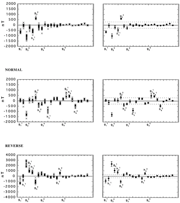
As noted by Johnson & Constable, and found by many researchers since Wilson (1970, 1971), the axial quadrupole

3.3 Uncertainties related to the data—influence of a g0

2is generally seen to be the dominant term in the inversion single site (see Section 4). Other apparently important terms (i.e.

signifi-After having checked the effects of using basically the cantly different from zero, given formal uncertainties and/or

same algorithm on the same data set, though with some spread of inverted results) are:

modifications, the next step was to analyse the effect of the contents of the data set itself. We therefore applied exactly (1) for the B data, the equatorial dipole g1

1(of the order of _{the same algorithm to subsets of the Q94 data set proposed} 60 per cent of g0

2), the h12and g22quadrupoles (50 per cent of _{by Quidelleur et al. (1994). Criteria for building that set were} g0

2) and possibly the g03axial octupole (30 per cent of g02); _{given in that paper, and were rather similar to those applied} (2) for the N data, h1

3 (70 per cent of g02) and to a lesser _{by Johnson & Constable (JC96) in their updated version of} extent g1

4, h14and h24(around 35 per cent of g02) and h22(30 per the Lee data set. There were some differences, however, which cent of g0

2); are summarized in the Appendix. This Appendix also provides (3) for the R data, g1

1, g12, h12, g22( between 35 and 50 per cent abbreviated codes for various versions of the data sets used of g0

2) and h11, h12, g03, g33and h33(15–20 per cent of g02). throughout this paper. The tests that follow have been per-formed on an updated, modified data set, Q94-m. We will first All other coefficients have either much smaller amplitude or _{illustrate problems resulting from individual data with} pre-a rpre-ange thpre-at includes zero. It mpre-ay be worth recpre-alling thpre-at,

viously unexplained or unspotted major effects, then resume although individual harmonic coefficients have no physical _{comparison with the JC95 results.}

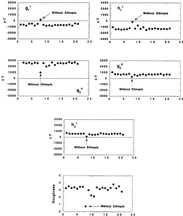
significance in themselves, they indicate the contribution of _{A striking effect is easily identified in a display of results} each individual spherical harmonic base function. Also, they _{from inverting the R data of the Q94-m data set, when a} jack-allow a comparison of the importance of zonal versus non- _{knife approach is applied to the data (Fig. 4). More precisely,} zonal, dipole versus non-dipole terms, or comparison of two _{the data set contains directions from 22 distinct geographical} different inversions. Only the total combination, however, gives _{sites. The jack-knife technique consists of performing the} a global view of the model and the quality of its fit to the data. _{inversion 22 times, removing all data from one and only one} Referring to Table 1(a), we can next compare the results given site at each time. Inspection of Fig. 4 shows that data obtained by JC95 with those that we derive. In this discussion, from a single site clearly perturb the inversion, this site being as in much of what follows, we use an arbitrary threshold of located in Ethiopia (Schult 1974). Unreasonably large values 300 nT, to be justified later, below which inverted model of g1

1, h11, g03 and h13 are obtained when the Ethiopian data are included, whereas all coefficients become smaller or even coefficients are not considered by us to be significantly different

Figure 3. Inverted spherical harmonic model coefficients up to degree and order 4 for the JC96-2 data (Johnson & Constable 1996; see Appendix), using the JC95 algorithm (Johnson & Constable 1995) as slightly modified and discussed in this paper (see text). Left side displays results from 10 inversions each, successively for the Brunhes, normal and reverse data subsets. Each inversion is based on the JC96 data set, adding to the published data random Gaussian noise compatible with revised values of uncertainties (see text). Right side displays corresponding mean values and standard deviations, emphasizing with dashed lines at±300 nT the range about zero in which it is argued that the model coefficients may not be significant. The maximum degree reached in the inversion is 4.

negligible when they are not. The amplitude of the axial with ages concentrated around 2 Myr, which has been dissected into rotating blocks by continental rifting and rift propagation quadrupole is also reduced by a factor in excess of 2. The

overall behaviour is particularly conspicuous in a graph of (Courtillot 1980; Tapponnier et al. 1990; Manighetti et al. 1997). This has resulted in heterogeneous rotations of blocks model roughness: this is 3–4 times less when the Ethiopian

data are excluded. The Schult (1974) data happen to come about vertical axes by up to 15°. As a result of this tectonic activity, these data cannot be included in a data set for the from a particularly complex and tectonically active area, the

Afar depression and triple junction, in which our group has purpose of geomagnetic analysis. New samples, collected south of the depression in the apparently unrotated termination of gathered extensive tectonic, palaeomagnetic and geochronologic

data over the past 15 years (Courtillot et al. 1984; Manighetti the East African Rift, should soon provide a more acceptable datum (Kidane et al., in preparation). The Ethiopian data are 1993; Manighetti et al. 1997; Kidane et al., in preparation). We

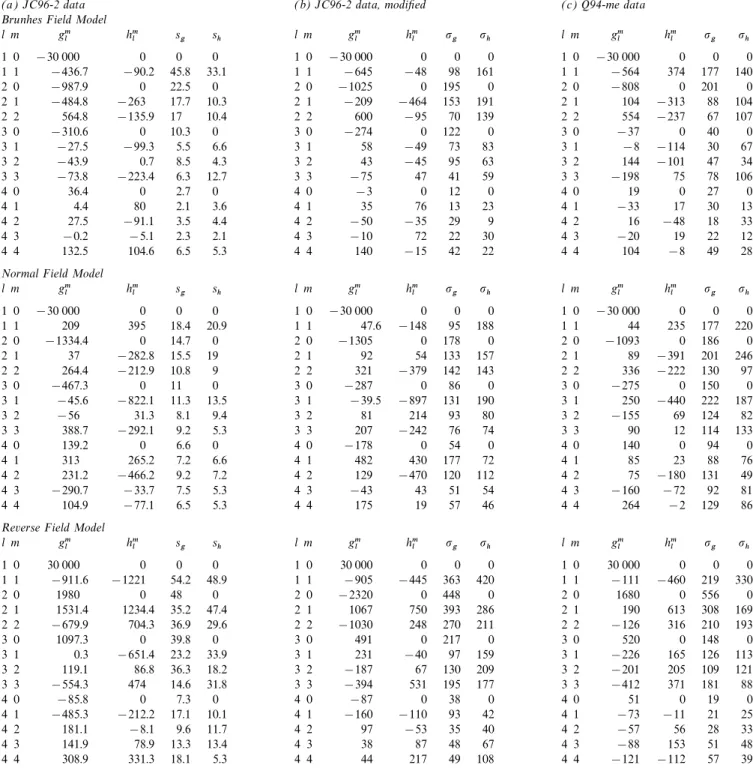
Table 1. Inverted field models for different sets of the Brunhes (B), normal (N) and reversed (R) data using the method of Johnson & Constable (1995) as modified and discussed in this paper. (a) Data from Johnson & Constable (1996, JC96-2), evaluation of standard errors S_gand S_hon gm_l and hm_l using a jack-knife approach. Maximum degree of inverted models set at 10. ( b) Data from Johnson & Constable (1996, JC96-2), with data uncertainties as modified in this paper (eqs 7 and 8) and standard deviations (s

gandsh) instead of standard errors. Maximum degree of inverted models set at 4. (c) Data from Quidelleur et al. (1994, Q94-me). Otherwise as in (b).

(a) JC96-2 data (b) JC96-2 data, modified (c) Q94-me data

Brunhes Field Model

l m gm_l hm_l s g sh l m gml hml sg sh l m gml hml sg sh 1 0 −30 000 0 0 0 1 0 −30 000 0 0 0 1 0 −30 000 0 0 0 1 1 −436.7 −90.2 45.8 33.1 1 1 −645 −48 98 161 1 1 −564 374 177 140 2 0 −987.9 0 22.5 0 2 0 −1025 0 195 0 2 0 −808 0 201 0 2 1 −484.8 −263 17.7 10.3 2 1 −209 −464 153 191 2 1 104 −313 88 104 2 2 564.8 −135.9 17 10.4 2 2 600 −95 70 139 2 2 554 −237 67 107 3 0 −310.6 0 10.3 0 3 0 −274 0 122 0 3 0 −37 0 40 0 3 1 −27.5 −99.3 5.5 6.6 3 1 58 −49 73 83 3 1 −8 −114 30 67 3 2 −43.9 0.7 8.5 4.3 3 2 43 −45 95 63 3 2 144 −101 47 34 3 3 −73.8 −223.4 6.3 12.7 3 3 −75 47 41 59 3 3 −198 75 78 106 4 0 36.4 0 2.7 0 4 0 −3 0 12 0 4 0 19 0 27 0 4 1 4.4 80 2.1 3.6 4 1 35 76 13 23 4 1 −33 17 30 13 4 2 27.5 −91.1 3.5 4.4 4 2 −50 −35 29 9 4 2 16 −48 18 33 4 3 −0.2 −5.1 2.3 2.1 4 3 −10 72 22 30 4 3 −20 19 22 12 4 4 132.5 104.6 6.5 5.3 4 4 140 ₋₁₅ 42 22 4 4 104 ₋₈ 49 28

Normal Field Model

l m gm_l hm_l s_g s_h l m gm_l hm_l s_g s_h l m gm_l hm_l s_g s_h 1 0 −30 000 0 0 0 1 0 −30 000 0 0 0 1 0 −30 000 0 0 0 1 1 209 395 18.4 20.9 1 1 47.6 −148 95 188 1 1 44 235 177 220 2 0 −1334.4 0 14.7 0 2 0 −1305 0 178 0 2 0 −1093 0 186 0 2 1 37 −282.8 15.5 19 2 1 92 54 133 157 2 1 89 −391 201 246 2 2 264.4 −212.9 10.8 9 2 2 321 −379 142 143 2 2 336 −222 130 97 3 0 −467.3 0 11 0 3 0 −287 0 86 0 3 0 −275 0 150 0 3 1 −45.6 −822.1 11.3 13.5 3 1 −39.5 −897 131 190 3 1 250 −440 222 187 3 2 −56 31.3 8.1 9.4 3 2 81 214 93 80 3 2 −155 69 124 82 3 3 388.7 −292.1 9.2 5.3 3 3 207 −242 76 74 3 3 90 12 114 133 4 0 139.2 0 6.6 0 4 0 −178 0 54 0 4 0 140 0 94 0 4 1 313 265.2 7.2 6.6 4 1 482 430 177 72 4 1 85 23 88 76 4 2 231.2 −466.2 9.2 7.2 4 2 129 −470 120 112 4 2 75 −180 131 49 4 3 −290.7 −33.7 7.5 5.3 4 3 −43 43 51 54 4 3 −160 −72 92 81 4 4 104.9 −77.1 6.5 5.3 4 4 175 19 57 46 4 4 264 −2 129 86

Reverse Field Model

l m gm_l hm_l s g sh l m gml hml sg sh l m gml hml sg sh 1 0 30 000 0 0 0 1 0 30 000 0 0 0 1 0 30 000 0 0 0 1 1 −911.6 −1221 54.2 48.9 1 1 −905 −445 363 420 1 1 −111 −460 219 330 2 0 1980 0 48 0 2 0 −2320 0 448 0 2 0 1680 0 556 0 2 1 1531.4 1234.4 35.2 47.4 2 1 1067 750 393 286 2 1 190 613 308 169 2 2 −679.9 704.3 36.9 29.6 2 2 −1030 248 270 211 2 2 −126 316 210 193 3 0 1097.3 0 39.8 0 3 0 491 0 217 0 3 0 520 0 148 0 3 1 0.3 −651.4 23.2 33.9 3 1 231 −40 97 159 3 1 −226 165 126 113 3 2 119.1 86.8 36.3 18.2 3 2 −187 67 130 209 3 2 −201 205 109 121 3 3 −554.3 474 14.6 31.8 3 3 −394 531 195 177 3 3 −412 371 181 88 4 0 −85.8 0 7.3 0 4 0 −87 0 38 0 4 0 51 0 19 0 4 1 −485.3 −212.2 17.1 10.1 4 1 −160 −110 93 42 4 1 −73 −11 21 25 4 2 181.1 −8.1 9.6 11.7 4 2 97 −53 35 40 4 2 −57 56 28 33 4 3 141.9 78.9 13.3 13.4 4 3 38 87 48 67 4 3 −88 153 51 48 4 4 308.9 331.3 18.1 5.3 4 4 44 217 49 108 4 4 _{−121 −112} 57 39

as illustrated by Fig. 4. However, many data come from active (data set Q94-me following the Appendix). This was done in the same way as JC96, and the results are shown in Fig. 5 and areas, and smaller yet significant tectonic effects might still

remain. Indeed, few of these palaeomagnetic sites have been listed in Table 1(c). Although the two data sets yield broadly similar results, particularly as regards the most important constrained by detailed tectonic analysis.

coefficients, it is interesting to point out a number of significant differences. In the discussion of ‘significant’ or ‘small’ coefficients, 3.4 Uncertainties in the data—the Q94 data set

we still retain the 300 nT threshold as a useful separator. Given that threshold, we find for the B data that g0

3 has Following the above observations, the inversion was

Figure 4. Selected inverted spherical harmonic coefficients (g1₁, h1₁, g0₂, g0₃and h1₃) using the modified Q94-m data set (see text and Appendix). Inversion is made by removing one site at a time ( jack-knife approach). There are 21 such inversions, number 8 corresponding to the case when the data from Ethiopia (Schult 1974) are removed. At the bottom is shown the evolution of model roughness during these tests.

On the other hand, h1

1, which was not significant in the JC96 become significant though not very large, and a couple have changed sign. This, or course, casts serious doubts on the data, becomes as significant as h1

2. Although still within the 300 nT band about zero, g3

3increases in amplitude. For the N robustness and actual geomagnetic meaning of these terms. data, the only term other than the axial quadrupole that was

quite large in the JC96 data, g1

3, has become reduced to the 3.5 Sources of data uncertainties edge of significance. It is particularly interesting that, in the N

data, all other terms now have uncertainties that include or A number of sources of uncertainty exist in the collection of palaeomagnetic samples and the production of remanence come very close to zero. In the R data, three previously

significant terms, g1

1, g12and g22, have now become insignificant. directions in the laboratory. These include orientation errors, undetected or uncorrected palaeoslope values and tectonic On the other hand, g3₃has become larger and g1₃has changed

sign (though on the edge of significance). rotations, and undetected and/or unremoved magnetic over-prints. Most palaeomagnetic data in the sets come from active Altogether, and limiting our analysis to degree and order 3

for the three data sets (B, N, R), six terms that were very volcanoes associated with hotspots. Although these often pro-duce fluid basaltic lavas, significant palaeoslopes may occur significant (i.e. larger than 800 nT) in the JC96 data have

Figure 5. Same as Fig. 3 for the modified Q94-me data set (see text and Appendix), with the data from Ethiopia removed (see Fig. 4).

have been measured and taken into account. The case for expected from a geocentric axial dipole. Fig. 1 from Tanaka et al. (1996) shows that most normal sites are located with the tectonic rotation can be particularly worrying; for instance, it

is reasonably well studied and understood in the Afar case, as Taupo Volcanic Zone, whereas the reversed ones tend to be located outside. We might therefore suggest that the heavily seen in the previous section, but smaller tectonic rotations in

the range normally attributed to secular variation may well faulted Taupo Volcanic Zone has undergone more tectonic deformation, resulting in rotations about vertical axes, than have gone undetected.

A recent example is given by Tanaka et al. (1996), who its surroundings. Hence, the reversed New Zealand data might be acceptable for PSV analysis, whereas the normal ones studied Brunhes- and Matuyama-age deposits from the central

Taupo Volcanic Zone in New Zealand. These authors find should probably be rejected. Further study of this is in progress (Tanaka et al. 1996).

what they believe to be otherwise correlative units yielding

divergent palaeomagnetic directions, which could be due either Another source of uncertainty, which we have analysed in a little more detail, stems from unremoved viscous or secondary to actual (fast, high-amplitude) palaeosecular variation (PSV),

or to extensional tectonics in this very active area. Strangely magnetic overprints. An increasing number of case studies indicate that such overprints may bias the directions of enough, the younger normal polarity sites appear to have

under-gone a clockwise rotation, whereas the older normal polarity what were otherwise thought to be clean primary remanence directions. This may be easy to detect when the directions of sites give a mean that is indistinguishable from the direction

the primary and secondary components are very different (e.g. Although such numerical experiments can only provide order-of-magnitude estimates, they cast very strong additional Vandamme et al. 1991), but becomes far more difficult when

they are similar. As an exercise, we have generated artificial doubts on the geomagnetic significance of terms other than g0

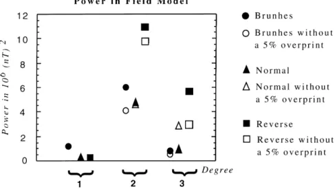
1 and g02. Returning to Fig. 6, we notice that the equatorial sets of B, N and R data by assuming that an overprint in

the direction of the present Earth’s field (actually the 1980 dipole, which is likely to be the easiest term to extract in the inversion, has the smallest amplitude. With a now generally IGRF) was still present in the Q94-me data set. We have

removed small vectors in the direction of the 1980 IGRF, accepted amplitude between 1000 and 2000 nT, g0 2 should contribute about 6×106 nT2 to the power of quadrupole assuming their amplitude to be 5 per cent of that of the natural

remanent magnetization (NRM). Rather than comparing each terms. This is the amplitude of the B and N power estimates. The largest power, almost double the expected value, is found individual coefficient, we evaluate the power in each one of

the first three degrees, using the Lowes (1974) formula: for the R data, i.e. the least well determined, the ones with the smallest data set and worst geographical distribution, the most R

l=(l+1) ∑ l m=0

[(gm

l)2+(hml)2] . (9) susceptible to the effect of overprints. Interestingly, the power in g0₂ decreases when one attempts to model the effect of The axial dipole is not included in the case l=1, where only overprinting. As far as the octupolar terms are concerned, the power related to the equatorial dipole is evaluated. Results are B and N data happen to yield a power similar to that in the shown in Fig. 6. Though they were already the smallest in equatorial dipole, i.e. quite low. The R data on the other hand amplitude, the equatorial dipole terms were least affected, have as much power as the quadrupole, but they are the most being orthogonal to the dominant g0

1, which is removed in affected by overprinting. Hence a large part of the power seen the modelled overprint. The l=2 terms were significantly in the inverted R models may result from a number of sources decreased in the case of the B and R data. For the l=3 terms, irrelevant to geomagnetic field modelling.

the R data led to the largest power reduction, whereas the N data led to an increase, B being hardly affected. Altogether,

3.6 Uncertainties related to site distribution removing a normal overprint led to a simpler field model with

less energy in the higher harmonics. This was clear for instance Many authors have mentioned the fact that the number of geographically separate sites was unfortunately small and their for the significant decrease of h1

3, leading one to suggest that

this might typically be an artefact of unremoved overprints distribution very heterogeneous. We are actually viewing the palaeofield through a particularly distorted spatial sampling (given the very oversimplified geometry of our overprint

model ). scheme (a sort of ‘antenna’) and this may naturally result in various forms of potentially serious aliasing. In Fig. 7, we have A similar exercise was performed by McElhinny, McFadden

& Merrill (1996). They assumed a fully zonal mean-field model mapped the average distance between each site and its neigh-bours (actually the arithmetic mean of the angular distance of and inverted the data in the form of the latitude distribution

of the inclination anomalies (departures from inclinations one site to all the other ones). For the B data, more than half of the Earth (the Pacific hemisphere) shows distances in excess predicted for a geocentric axial dipole). They generated a field

model with only g0

1 and g02 contributions at the actual sites of 60°. For the R data, this applies to all of the Earth, except locally near Europe, North Africa and the North-East Atlantic. of the data set, injected a 5 per cent normal overprint and

inverted the resulting ‘observations’. A g0

3 with an amplitude This would in itself (a priori) raise doubts as to the possibility of extracting valid global estimates of harmonics with degree comparable with g0

2was found, which could only be an artefact.

Figure 6. Power spectrum of each inverted field model for the first three degrees using the Lowes (1974) formula. The axial dipole g0₁has been excluded when calculating power in the n=1 terms. Full symbols are for data from the Q94-me data set (see Appendix), for the Brunhes, normal and reversed subsets. Open symbols are for the same data after removal of a present-day normal overprint (IGRF 1980) with amplitude equal to 5 per cent of the NRM.

Figure 7. Average angular distance in degrees between any site and all of its neighbours for the Brunhes ( B), normal (N) and reversed (R) subsets of data from Q94-me (see Appendix).

equal to or in excess of 3. The areas with denser sites may of the exact site locations where data are available for each subset, and inverted them up to degree and order 3. This is a course lead to aliasing in less well constrained zones (i.e. the

majority of the Earth’s surface in all cases but the N data, for simple way of investigating the cross-correlation of model param-eters in the inversion. The maximum values of non-diagonal which average spacing is everywhere between 40° and 55°).

The influence of site distribution can be tested in various terms are of the order of 0.1 mT and can reach 0.2 mT. For example, a 1 mT g0₂in the B site distribution generates through ways. A simple way is to generate artificial data for simple

field models, invert them and compare the results to the input. aliasing equatorial dipole components g1

1=92 nT and h11= 123 nT, and also h2

2=76 nT and h23=74 nT. A 1 mT g12(in the In this way, we have generated seven field models, each of

which involves a constant axial dipole (g0

1=30 mT) and a N site distribution) generates g11=178 nT, g02=85 nT, g13= 72 nT, … . In addition, note that the diagonal term that is single other term of 1 mT amplitude, going up to degree and

synthetic data) is itself recovered with an error ranging from Thus, these inversions strongly suggest that only g0 1and g02 may be sufficiently robust to the various changes in method, −200 to −400 nT (always with the same sign, that is an

data set, etc. Therefore, a model where only these two axial underestimate by up to 40 per cent).

terms are non-zero and all other coefficients do average out to zero appears to be consistent with the data and the con-fidence we can place in them. This is essentially the structure 4 D I S C U SS I O N A N D C O N C L U SI O N S _{of the CP88 (Constable & Parker 1988) giant Gaussian process,} recently further explored by Quidelleur & Courtillot (1996). Courtillot et al. (1992) argued that, given data quality and

We will return later to its variance structure. remaining differences between models, it seemed difficult to

As noted before, McElhinny et al. (1996) have recently demonstrate that the long-term (1 Myr) average geomagnetic

explored a complete palaeomagnetic database. They argue, field contained any persistent feature beyond the g0

1 axial based on declination anomalies, for the lack of significance of dipole. The rest appeared to behave like random noise, the

any non-zonal variations, but fail to explore this in a systematic present-day non-axial-dipole field being a typical sample of this

way. However, our own results provide a firmer basis for this random noise. However, further work by many authors has

proposal. Our study leads us to confirm that the g0

2/g01ratio is confirmed the presence of a small persistent axial quadrupole

of the order of 4 per cent, ranging from 3.5 to 5.5 per cent. g0

2, first discovered by Wilson (1971). However, all other terms Original estimates by Merrill & McElhinny (1997) were in the remain a matter of controversy. _{range of 5 to 8 per cent, estimates based on} sedi-We can use the various results from the previous sections to _{mentary data from 3 to 5 per cent (Schneider & Kent 1988).} place further constraints on those. The exercise leading to the _{The recent analysis of inclination anomalies by McElhinny} calculation of influence matrices has shown that, all other _{et al. (1996) leads to 3 to 4 per cent. These values are in rough} features being constant, a 1 mT quadrupole would alias into _{agreement, with the more recent ones tending to be on the} other components, most notably the equatorial dipole with _{lower side of earlier ranges. Taking arbitrarily a mean value} amplitudes of the order of 0.1 to 0.2 mT. This is largely due to _{for the axial dipole of the order of 30 mT would lead to an} the very inhomogeneous distribution of the approximately 20 _{axial quadrupole between 1 and 1.5 mT. The above analysis} sites where data are available. Comparing results from inver- fails to provide convincing support, again within current sions performed by various authors on various data sets (e.g. uncertainties in the data, for other persistent features (such as Gubbins & Kelly 1993; JC95; this paper), and comparing an axial octupole g0₃), or for north versus south hemispherical within the same study inversion of B, N and R type data, give asymmetry or for normal versus reversed polarity asymmetry. A contentious issue is that of the persistence of higher-latitude a further idea of the threshold under which individual terms

flux concentrations (Gubbins & Kelly 1993). We do not cannot be considered as significantly different from zero. As a

observe such features, though our maximum degree of 4 may matter of convenience, we propose that this threshold is of the

not be sufficient for their identification. We note, however, order of±0.3 mT. This is taken to represent the rough limit of

that, as data quality and methods progress, these become less resolution beneath which it is difficult to decide whether a

and less apparent (see note added in proof at the end of coefficient has real significance or is just an artefact.

the paper). Given that threshold, very few terms stand out clearly in a

We can use our preferred model to generate maps of the robust fashion. The g1₁equatorial dipole for instance is reduced

mean field, which can be compared to the original data (D, I), when one goes from the Johnson & Constable data set (Fig. 3)

or continued downwards at the CMB. Examples of the latter to ours (Fig. 5), and is completely absent in the N and R data.

for the radial (vertical) component B

rare shown in Fig. 8. Not It is therefore reasonable to assume that the geomagnetic

surprisingly, our maps tend to be smoother than (though quite equatorial dipole averages to zero over these timescales

similar to) those of JC95 actually generated after removal of (consistent with all ideas in dynamo models regarding the role

‘anomalous’ sites (their Figs 13–15, models LB2, LN2 of Coriolis force), and that it does not average out in our B

and LR2). This is particularly true for the reversed data. data because of, for instance, poor site distribution or

remain-Oscillations or features tend to appear in areas with the least ing recent overprints. Also, a g2

2term of about 0.6 mT appears constraints, i.e. the Southern Hemisphere and the Pacific in the B data (for both the Q94-me and JC96-2 data sets), but

Ocean. For the B data, the magnetic equators we find fluctuate is at or below the 0.3 mT threshold in the N or R data. There

about the geographic equator, but they are not in phase is also a h1

3term of−0.6 mT in the N data, but in neither the between the JC96 (LB2) and our model. For the N data, JC96 B nor the R data. It is this h1

3 term which suffers the largest (LN2) have complex features that we do not see in the Pacific reduction when going from the JC96 to the Q94 data set. As _{between Hawaii and Tahiti. Recall, however, that our inversion} noted above, three terms in the R model that appeared in the _{is stopped at n=4, whereas JC95 calculate models up to} JC96 results (g1

1, g12 and g22) are not significant any more in degree and order 10. our results. Finally, if we check which coefficients (except g0

2) Declination and inclination anomalies (with respect to are both significant and common to the two data sets, we find _{the pure axial dipole model ) are of potential interest in a} only g2

2 and g11 for the Bunhes data, and h12 and g03 for the number of palaeomagnetic applications. Again, it is interesting reverse data. These terms should therefore be the prime _{that inclination anomalies (Fig. 9) do not exceed about 3°} candidates for further testing of robustness and significance. near where data are actually constraining the model. For the Given the tests of McElhinny et al. (1996), not much confidence Brunhes data, the anomaly reaches−4° in New Zealand, and for instance can be placed on the reality of any g0

3. If we add the strong (−9°) anomaly in the western–central Pacific is the condition that coefficients should belong to all three data entirely unconstrained by local data; 16 out of 20 sites have DI less than 2°. Anomalies tend to be smaller (due to more subsets, only g0

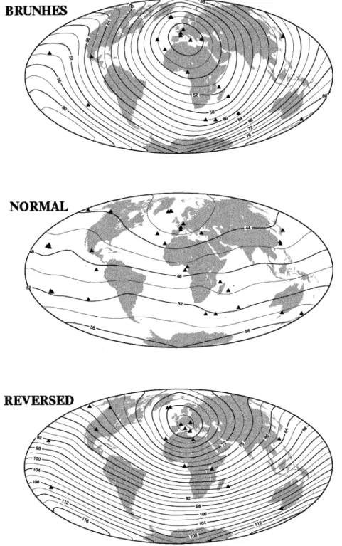
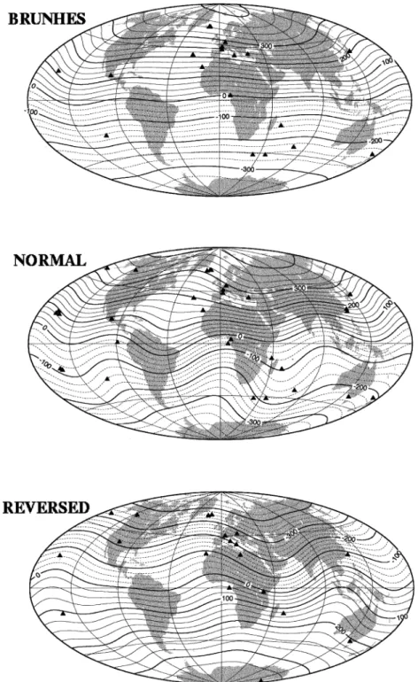
Figure 8. Average field model resulting from the inversion of the Q94-me Brunhes ( B), normal (N) and reversed ( R) data up to degree 4 (see Appendix). This is shown as a map of the radial component B_rat the core–mantle boundary. Contour interval is 25 mT. Triangles show sites where data are available.

sites, or better distribution, or better averaging, etc.) for the N is no evidence for large regional anomalies as have been hypothesized to explain some awkward palaeomagnetic data. Values of −4° are reached only in West Africa and

Hawaii, and again a large (−7°) anomaly centred on Indonesia data—for instance in Asia in the Tertiary by Westphal (1993). It is clear that the simple (g0

1, g02) model could possibly be is actually not locally constrained; 17 out of 31 sites have DI

less than 2°. The inclination anomaly map for the R data invalidated by more numerous, better distributed, or more accurate and representative data and complementary inversion appears much more rugged but actually, apart from China

(8°), Hawaii (6°) and West Africa (7°), all sites show values techniques. The above results can be used to point out the directions in which it might next be desirable to go.

less than 4–5°, often less than 3°. Declination anomalies

are mostly less than 2°, and always less than 4° at all sites, For one thing, the inverse technique of Johnson & Constable (1995) used throughout the present study makes simplifying except at the higher latitudes. We note in passing that there

Figure 9. Maps of inclination anomalies (inclination corresponding to each field model from Fig. 8, minus inclination predicted for geocentric axial dipole), in degrees. Same format as Fig. 8.

assumptions as to the variance structure of the giant Gaussian with an inverse problem formulation based on theoretical descriptions and formulae of Kono & Tanaka (1995b) and process. Recent work, using various average distributions

extracted from the data sets, has emphasized that, contrary to Hulot & Gallet (1996) might allow one to go further and test the joint uncertainties of what appears today to be the most the hypotheses of Constable & Parker (1988, hereafter CP88),

the variance of terms of a given degree may also depend on appealing and simplest model: a CP88-like giant Gaussian process with only one added free parameter (namelys1

2). It order. Quidelleur & Courtillot (1996) have shown that a larger

value of s1₂, the variance of the degree-2 and order-1 non- would remain to understand whether this new parameter actually provides information on the field generating process zonal quadrupole, was sufficient to account for much of the

remaining misfit to the data set. Kono & Tanaka (1995b) and or remains an artefact due to data distribution.

Another predictive benefit of the inverse approach further Hulot & Gallet (1996) have provided a theoretical basis to

understand the importance of order m=1 terms. Combining discussed in this paper is to test how the situation could be improved by collecting more, better or other data. For instance, the distributions displayed by Quidelleur & Courtillot (1996)

one could test how acquisition of new PSV data from ill- the axial dipole and quadrupole. Asymmetries between the Northern and Southern Hemispheres, or between the normal sampled areas could alleviate some non-uniqueness. The

geometry of the actual site distribution, this unavoidable spatial and reversed states, are not yet resolvable. The most puzzling feature to be further analysed is the dependence of the variance filter through which the core field must be viewed, is unlikely

to change much in the near future. Indeed, this is a map of of the various terms not only on degree but also on order, with the prominence of the order-1 quadrupolar variance. the main sources of abundant recent volcanism, mainly

hot-spots, sufficiently remote from major tectonic disturbance. We have seen the major and adverse influence of sites such as

N O T E A D D E D I N PR O O F Ethiopia, where tectonic rotations had not been properly

assessed. There has been since 1995 a healthy interaction between our group and the team formed by Catherine Johnson and Clearly, new data from the central Pacific or southern

Atlantic (e.g. Tristan da Cunha) would be extremely interesting. Catherine Constable. The latest results of this are a set of two papers, the present one and a new one by Johnson & Constable We should point out, however, that further sampling in areas

where data are already available could be essential too. For (1997, hereafter JC97). The two papers were submitted to this journal respectively in December 1996 and January 1997. As instance, there are three sites within 50 km of each other in

Reunion Island in the Indian Ocean that have yielded very might be expected, the senior authors were among the reviewers of the other’s paper. Acceptance of JC97, and exchanges at the discrepant inclination values of respectively −38.9°±2.8°,

−29.1°±5.3° and −47.6°±1.6° (uncertainties are s_I calcu- time of review, led us to this note added in proof in November 1997, which may be a useful complement to the main body of lated from the orginal data and augmented by 10 per cent

as outlined in a previous section). Such values cannot be our paper.

The improvements and/or additions of JC97 over JC95 accounted for by the same low-order mean-field model.

Problems linked to tectonics, palaeoslopes and incomplete include the correction in the standard errors that was pointed out in Section 2.1. Also the lava data base is sifted and a removal of overprints could all have contributed, and further

data from Reunion are clearly needed. number of data are eliminated on the basis of a number of potential problems and limitations. Data sets are averaged Vandamme et al. (1991) have shown, in the case of another

large data set, that of lava flows from the Deccan traps in within 5° spatial bins. Finally, sediment data are included. JC97 use linearized data Green’s kernels to demonstrate how India, that improvement in palaeomagnetic techniques as time

progressed was apparent in the data. Variances calculated with declination and inclination data sample the core–mantle boundary; they argue that adding sediment to lava flow data and without measurements made prior to 1980 were

signifi-cantly different. Indeed, introduction of cryogenic magnet- improves CMB coverage.

In their new paper, JC97 reach a number of conclusions ometers and better (and more systematic) magnetic cleaning

and interpretation techniques for extracting primary magnetiz- that differ from their JC95 views and come very close to our own results (see also Carlut & Courtillot 1995, 1996). JC97’s ation directions make post-1980 data in general far more

reliable. However, applying this criterion to the Q94 data set new inverted models, like ours, incorporate a number of modifications and it is not always straightforward to evaluate would reduce the number of data and site averages even further

and make the inversion virtually impossible. For instance, the effects of single changes (data sifting, uncertainty modi-fication, different data binning, inclusion of sedimentary data). selecting only those data involving proper cleaning and

demagnetization (which implies rejection of undemagnetized But it is interesting that their final models are very significantly smoother than their JC95 results. When heavier smoothing NRM-only directions and blanket demagnetizations without

vector diagrams) reduces the number of available, distinct sites constraints (norms) are used, the results are very similar to ours indeed. JC97 conclude, as we did, that much of the structure in the Brunhes data from 20 to five! This clearly implies that

inversion with data meeting now generally accepted quality found in their previous models (JC95) can be attributed to sites with poor temporal sampling. Sediments (which, as stated criteria is still not possible. In any case, seriously

underesti-mated published data uncertainties and various remaining above, we believe should probably not be used) are found not to contribute much structure. The high-latitude flux lobes are sources of bias discussed in this paper underline the necessity

of bringing detailed knowledge of what palaeomagnetic sam- not observed, and JC97 conclude, like us, that they cannot be detected given the quality and distribution of current data sets. pling, laboratory measurement and data interpretation actually

amount to, into any long-term mean-field analysis. Once these The main feature on which we and JC97 would still differ is the significance of the non-zonal part of the field. The reality have been sufficiently advanced, it will be useful to attempt to

include sedimentary data and also palaeointensity data into of a major anomalous feature in the Pacific Ocean would require further checking (it appears only when the maximum the inversion. We believe, however, that the number and

quality of much data and our understanding of whether they degree of the inversion is high—i.e. our Fig. 2b). But like us, JC97 now conclude that flux lobes in other models result from actually represent accurate pictures of the palaeofield at the

kind of space and time resolution we are seeking for PSV overprinting, that polarity asymmetries cannot be resolved, and that some of the data in existing databases need to be analysis do not as yet allow them to be usefully incorporated

into the PSV data set of lava flow palaeomagnetic directions. updated and complemented by further work: in other words, a number of data are probably affected by significant undetected As pointed out above, a lot of homework (obtaining new

directional data from both new and old sites) needs to be errors, and proper palaeomagnetic analysis of each datum is required (and often not even sufficient to uncover the sources accumulated.

In conclusion, our belief is that available data do not require of anomalies).

We also wish to point the reader’s attention to another a more complex model than one in which the only non-zero