HAL Id: hal-00316668
https://hal.archives-ouvertes.fr/hal-00316668
Submitted on 1 Jan 1999
HAL is a multi-disciplinary open access
archive for the deposit and dissemination of sci-entific research documents, whether they are pub-lished or not. The documents may come from teaching and research institutions in France or abroad, or from public or private research centers.
L’archive ouverte pluridisciplinaire HAL, est destinée au dépôt et à la diffusion de documents scientifiques de niveau recherche, publiés ou non, émanant des établissements d’enseignement et de recherche français ou étrangers, des laboratoires publics ou privés.
Letter to the Editor: Spatial and seasonal variations of
the foF2 long-term trends
A. D. Danilov, A. V. Mikhailov
To cite this version:
A. D. Danilov, A. V. Mikhailov. Letter to the Editor: Spatial and seasonal variations of the foF2 long-term trends. Annales Geophysicae, European Geosciences Union, 1999, 17 (9), pp.1239-1243. �hal-00316668�
Letter to the editor
Spatial and seasonal variations of the foF2 long-term trends
A. D. Danilov1, A. V. Mikhailov2
1Institute of Applied Geophysics, Rostokinskaya 9, Moscow 129128, Russia
2Institute of Terrestrial Magnetism, Ionosphere and Radio Wave Propagation, Troitsk, Moscow Region 142092, Russia
Received: 19 March 1999 / Accepted 29 March 1999
Abstract. Using a method suggested by the authors earlier, the long-term trends of the F2-layer critical frequency, foF2 are derived for a set of ionospheric stations with a wide latitudinal and longitudinal cover-age. All the trends are found to be negative. A pronounced dependence on geomagnetic latitude is found, the trend magnitude increasing with the latter. No globe scale longitudinal eect in trends is detected. For the majority of the stations there is also a pronounced seasonal eect, the trend magnitude being higher in summer than in winter.
Key words. Ionosphere (ionospheric disturbances; mid-latitude ionosphere)
1 Introduction
There is an interest in the problem of long-term variations (trends) in the upper atmosphere parameters (see reviews by Danilov (1997, 1998). Trends of the ionospheric F2-region parameters were considered in several papers, e.g. by Givishvili and Leshchenko (1994, 1995), Bremer (1996), Ulich and Turunen (1997), Danilov and Mikhailov (1998), Bencze et al. (1998), Jarvis et al. (1998). Recently a detailed consideration of the trends in the ionospheric E, F1 and F2 regions was presented by Bremer (1998).
Danilov and Mikhailov (1998) proposed a new approach to revealing the foF2 trends. With this new approach, the authors obtained negative trends for all four ionospheric stations considered and some indica-tions to the existence of a latitudinal eect, the magni-tude to the negative trend increasing with latimagni-tude. Contrary to that Bremer (1998), analyzing foF2 trends
for European ionospheric stations, obtained dierent signs of the trend for dierent groups of stations (some sort of a longitudinal eect) and detected no latitudinal variation. This contradiction is discussed below.
In this paper, further analysis of the foF2 data in the scope of the new approach proposed by the authors is performed with an accent on spatial and seasonal variations of the trends.
2 Method and data
The method proposed by Danilov and Mikhailov (1998) is based on the following:
1. Relative deviations of the observed foF2 values from some model
dfoF2 foF2 obsÿ foF2mod=foF2mod 1
are analyzed instead of absolute values considered by Givishvili and Leshchenko (1994, 1995) and Bremer (1996, 1998). The advantage of using relative values instead of absolute ones are discussed by Danilov and Mikhailov (1998). A third-degree polynomial in respect to the sunspot number R12 is used as a model:
foF2 a0 a1X a2X2 a3X3 2
where X = R12and coecients aiare found by the least
squares method.
2. A 12-month running mean foF2 rather than monthly values are used for the analysis.
3. Only three years around solar maxima and minima [M(3) + m(3)] are considered to reveal foF2 trends. This is done to get rid of the hysteresis eect which may be strong during the rising and falling phases of solar cycle and distorts the long-term variations sought for. In fact [see Danilov and Mikhailov (1998) for details] using only the M(3) + m(3) years it is possible to obtain stable negative trends, whereas for all years (including rising and falling phases) there is a chaos with various signs of the trends obtained on various stations.
Correspondence to: A. D. Danilov e-mail: [email protected]
4. Trends at dierent stations may be compared only if one and the same time period is taken for the analysis. A period 1965±1990 is the most rich with observations over the worldwide ionosonde network. Moreover it was shown by Danilov and Mikhailov (1998) that the most stable picture of the trends for all months and all the stations considered is observed if only the data since 1965 are analyzed. This seems quite reasonable if the trends in question are by this or that way related to anthropogenic eects. That is why in the present study we used the M(3) + m(3) data for 1965±1990 for all the stations considered. On the other hand, it should be stressed that the model (foF2 versus R12 regression) is
derived over all foF2 observations available on a particular ionosonde station.
5. Gaps in the initial observational data are ®lled in using the monthly median MQMF2 model by Mi-khailov et al. (1996) based on a new ionospheric index MF2 (Mikhailov and Mikhailov, 1995). This index may be applied for monthly median foF2 modelling over the whole northern hemisphere, so this approach was used for all the stations in question. All foF2 observations (given in zonal or UT time) were converted to solar local time using spline-interpolation. Only the data for 1200 SLT were used in the present analysis.
3 Spatial variations
Ground-based ionosonde observations over Europe, North America and Asia were used in this study. The
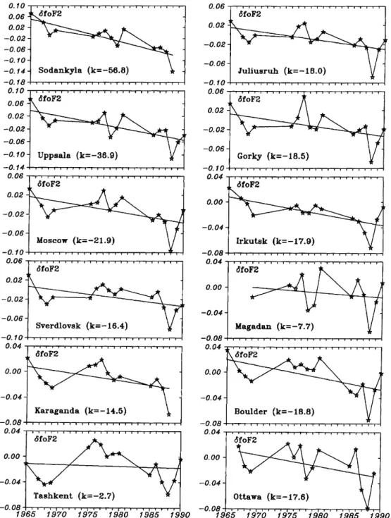
Fig. 1. The dfoF2 values versus a year for dierent latitudes (left-hand panel) and longitudes (right-hand panel) for April. The slope k of the regression line is shown in
10)4units/per year
1240 A. D. Danilov, A. V. Mikhailov: Spatial and seasonal variations of the foF2 long-term trends
LE
TT
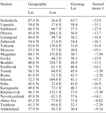
station list is given in Table 1. The stations are named as they were called in the period of observations. Table 1 shows that there is a broad coverage of the latitudes (both geographic and geomagnetic) and longitudes which provides the possibility of studying spatial variations of the eect in question.
An example of latitudinal (left-hand side) and longi-tudinal (right-hand side) dfoF2 behaviour for one month (April) is given in Fig. 1. One can see that for the data chosen, according to the principles described above, there are negative trends for all stations. All the trends are signi®cant with the con®dence level not less than 95% using the Fisher's criterion. Slope k (in 10)4 units
per year) of the regression line is given in Fig. 1 for each station. Negative foF2 trends are seen in annual mean k values as well (Table 1). An obvious latitudinal depen-dence for the slope k (a pronounced decrease) takes place when we move from high-latitude stations to low-latitude ones.
A dependence of April and annual mean absolute k values on geomagnetic latitude is shown in Fig. 2 for all stations in question. A dierence by more than an order of magnitude in k values is seen when high- and low-latitude stations are compared.
An analysis has shown that the k dependence on geomagnetic latitude is more pronounced than on geographic latitude. So a geomagnetic control of trend magnitude dominates over the geographic one. Indeed, the stations with similar geomagnetic but dierent geographic latitudes (e.g. Sverdlovsk, kaver=
)14.2 ´ 10)4 and Boulder, k
aver= )15.5 ´ 10)4) give
close values of k averaged over a year and vice versa the stations with close geographic latitude but dierent geomagnetic latitude ± for example, Ottawa (kaver=
)13.7 ´ 10)4) and Alma-Ata (k
aver= )0.82 ´ 10)4)
give strongly dierent values of the trend. This is a general tendency, but exceptions are possible as well (see Table 1). For example, Yakutsk has a very large k corresponding to higher latitude stations, while Maga-dan, Tomsk, Rome with relatively high geomagnetic latitudes have too low k values. Novokazalinsk and Ottawa with close geographic latitudes but quite dierent geomagnetic have close k values.
Longitudinal variations of k values are given in Fig. 1 (right hand side) for stations with geomagnetic latitudes U = 41.57° . All of them except for Magadan have close k around - 18 ´ 10)4. This manifests the absence of
global scale strong longitudinal variations in foF2 trends at least for midlatitude stations. But additional analysis of longitudinal variations is needed. Apart from the problem with Magaden, Irkutsk with relatively low geomagnetic latitude U = 41.06° demonstrates as large trend as Ottawa (U = 56.78°) does. This means that besides geomagnetic control some additional factors are responsible for the observed foF2 trends.
4 Seasonal variations
Using the 12-month running mean values of both sunspot numbers and F2 critical frequencies Danilov
Table 1. Ionosonde stations and calculated annual mean slope k
(in 10)4units/per year)
Station Geographic Geomag
Lat Annualmean k
Lat Lon Sodankyla 67.4 N 26.6 E 63.7 )53.9 Uppsala 59.8 N 17.6 E 58.4 )31.1 Salekhard 66.5 N 66.7 E 57.3 )27.9 Ottawa 45.4 N 284.1 E 56.8 )13.7 Leningrad 60.0 N 30.7 E 56.2 )18.8 Julinsruh 54.6 N 13.4 E 54.4 )16.1 Yakutsk 62.0 N 129.6 E 51.0 )31.0 Moscow 55.5 N 37.3 E 50.8 )19.1 Magadan 60.1 N 151.0 E 50.7 )7.94 Gorky 56.1 N 44.3 E 50.3 )15.9 Boulder 40.0 N 254.7 E 48.9 )15.5 Svedlovsk 56.7 N 61.1 E 48.4 )14.2 Tomsk 56.5 N 84.9 E 45.9 )3.39 Rome 41.9 N 12.5 E 42.5 )2.58 Irkutsk 52.5 N 104.0 E 41.1 )15.3 So®a 42.6 N 23.4 E 41.0 )16.9 Karaganda 49.8 N 73.1 E 40.3 )11.6 Khabarovsk 48.5 N 135.1 E 37.9 )5.39 Novokazalinsk 45.8 N 62.1 E 37.6 )14.1 Alma-Ata 43.2 N 77.0 E 33.4 )0.82 Tashkent 41.3 N 69.6 E 32.3 )2.29 Ashkhabad 37.9 N 58.3 E 30.4 )9.14
Fig. 2. The April (top box) and annual mean (bottom) log k values versus geomagnetic latitude
LE
TT
and Mikhailov (1998b) expected that there should be no month-to-month variations of the trend. But the present analysis demonstrates that there do exist seasonal variations of k. Fig. 3 shows typical annual variations of k values for high, middle, and low latitude stations. Annual variations are well pronounced at all latitudes with an increase to low ones. At high-latitudes the largest negative foF2 trends take place around the vernal equinox and the smallest ± in October-November with the amplitude range of 1.3±2.2. At middle and low latitudes the largest negative trends are observed in spring-summer months and the smallest trends take place in winter. The magnitude of seasonal variation is a factor of 2 at middle latitudes and larger for low-latitude stations. For stations with small trends (Rome, Alma-Ata, Tashkent, Tomsk) the sign of the trend turns out to
be even positive in winter months. One hardly may consider these positive values of k as signi®cant because they are small enough. On the other hand this eect may have physical origin keeping in mind a geomagnetic control of the trend magnitude (Fig. 2) and its possible relationship with geomagnetic disturbances.
5 Discussion
The method proposed by the authors earlier is applied to more data of the vertical ionospheric sounding. If all the years for which the data are available are considered, the trends may be of any sign and amplitude with no systematic dependence on the latitude. For example, at Tomsk for 1946±1995 the April k is negative
Fig. 3. Annual variations of k for high, middle, and low latitude ionospheric stations
1242 A. D. Danilov, A. V. Mikhailov: Spatial and seasonal variations of the foF2 long-term trends
LE
TT
()3.0 ´ 10)4), whereas at Moscow for the same years k
is positive (+0.92 ´ 10)4). A strong negative trend
(k = )12.4 ´ 10)4) may be found over 1949±1991 at
Irkutsk, whereas a positive (k = +0.12 ´ 10)4) trend
takes place at Leningard for 1950±1992. Some system in the k values appears only if the M(3) + m(3) years after 1965 are used. Then the values of k averaged over the year are negative for all the stations considered. There also appears to be some system in the latitudinal dependence of k illustrated by Fig. 2 and Table 1 with a pronounced decrease of the trend magnitude towards lower geomagnetic latitudes. The trends demonstrate also seasonal variations with a tendency to decrease in the summer months (see ®g. 3).
It should be stressed that our conclusions contradict those in the recent publication by Bremer (1998). He found no latitudinal eect in the trends, but detected some separation of the stations to two longitudinal groups with positive trends in Eastern Europe and negative ones in Western Europe.
We believe that the reason for the above contradic-tion lies in the dierences of the approaches used by Bremer (1998) and in this paper. Bremer used absolute deviations from some model (which describes the dependence of foF2 on solar and geomagnetic activity) and all the years available for a given station. In this case the length of the data series used is inevitably quite dierent depending on the duration of the vertical sounding observations at this particular ionosonde. The most important point is the hysteresis eect at the rising and falling phases of the solar cycle which may completely distort real long-term trends. We get rid of this eect by limiting our consideration with the M(3) + m(3) years.
Thus, the results of this paper con®rm our previous conclusions on the negative trends of foF2 since 1965. The origin of the trends is still a matter of discussion. Danilov and Mikhailov (1998) showed that the combi-nation of the data on the trends in foF2 and hmF2 (the height of the F2-layer maximum) leads to some sugges-tions on possible mechanisms responsible for these trends and related these mechanisms with a systematic increase in downward plasma drift velocity and/or atomic oxygen content decrease.
The foF2 latitudinal dependence derived in this study (especially the fact that the latitude in question is the geomagnetic one) do not contradict the above mecha-nism but trends to suggest further that the mechamecha-nism may be in some way related to ionospheric disturbances (ionospheric storms) following geomagnetic storms. The seasonal dependence may be a manifestation of the same process because it is well known that there are seasonal eects in occurrence and development of ionospheric storms (see e.g. ProÈlss, 1995). It is worth mentioning that
there are indications to some long-term trends in the occurrence frequency of ionospheric storms [see Serge-enko and Kuleshova (1994, 1995)]. Anyway, the question on the physical mechanisms of the foF2 trends is still open and hopefully the results of this paper provide some ground for further consideration of the problem.
Acknowledgements. Topical Editor D. Alcayde thanks H. Rish-berh for his help in evaluating this paper.
References
Bencze, P., G. Sole, L. F. Alberca, and A. Poor, Long-term changes of hmF2: possible latitudinal and regional variations, Proceed-ings of the 2nd COST 251 Workshop ``Algorithms and models for COST 251 Final Product'', 30±31 March, 1998, Side, Rutherford Appleton Laboratory, UK, 107±113, 1998.
Bremer, J., Some additional results of long-term trends in vertical incidence data, Paper presented at the COST 251 Meeting, Prague, September 1996.
Bremer, J., Trends in the ionospheric E and F regions over Europe, Ann. Geophys., 16, 986±996, 1998.
Danilov, A. D., Long-term changes of the mesosphere and lower thermosphere temperature and composition, Adv. Space Res., 20, 2137±2147, 1997.
Danilov, A. D., Review of long-term trends in the upper mesosphere, thermosphere and ionosphere, Adv. Space Res., 22, 907±915, 1998.
Danilov, A. D., and A. V. Mikhailov, Long-term trends of the F2-layer critical frequencies: new approach, Proceedings of the 2nd COST 251 Workshop ``Algorithms and models for COST 251 Final Product'', 30±31 March, 1998, Side, Turkey, Rutherford Appleton Lab., UK, 114±121, 1998.
Givishvili, G. V., and L. N. Leshchenko, Possible proofs of presence of technogenic impact on the midlatitude ionosphere, Doklady RAN, 334, 213±214, 1994 (in Russian).
Givishvili, G. V., and L. N. Leshchenko, Dynamics of the climatic trends in the midlatitude ionosphere E region, Geomag. and Aeron., 35, (3), 166±173, 1995 (in Russian).
Jarvis, M. J., B. Jenkins, and G. A. Rodgers, Southern hemisphere observations of a long-term decrease in F region altitude and thermospheric wind providing possible evidence for global thermospheric cooling, J. Geophys. Res., 103, 775± 20, 787, 1998.
Mikhailov, A. V., and V. V. Mikhailov, A new ionospheric index MF2, Adv. Space Res., 5, 93±98, 1995.
Mikhailov, A. V., V. V. Mikhailov, and M. G. Skoblin, Monthly median foF2 and M(3000)F2 ionospheric model over Europe, Ann. Geo®sica, 39, 791±805, 1996.
ProÈlss, G., Ionospheric F-region storms, in Handbook of Atmo-spheric Electrodynamics, v. 2, Ed. H. Volland, CRC Press, Press/Boca Raton, 195±248, 1995.
Sergeenko, N.P., and V.P. Kuleshova, Climatic changes of the properties of disturbances in the ionosphere and upper atmo-sphere, Doklady RAN 334, 534±536, 1994.
Sergeenko, N. P., and V. P. Kuleshova, Long-term trends of the F2 layer ionospheric disturbances, Geomagn. and Aeron., 35, 128± 130, 1995 (in Russian).
Ulich, T., and E. Turunen, Evidence for long-term cooling of the upper atmosphere in ionospheric data, Geophys. Res. Lett., 24, 1103±1106, 1997.
LE
TT