HAL Id: hal-03209761
https://hal.archives-ouvertes.fr/hal-03209761
Submitted on 28 Apr 2021
HAL is a multi-disciplinary open access
archive for the deposit and dissemination of
sci-entific research documents, whether they are
pub-lished or not. The documents may come from
teaching and research institutions in France or
abroad, or from public or private research centers.
L’archive ouverte pluridisciplinaire HAL, est
destinée au dépôt et à la diffusion de documents
scientifiques de niveau recherche, publiés ou non,
émanant des établissements d’enseignement et de
recherche français ou étrangers, des laboratoires
publics ou privés.
δ18O water isotope in the iLOVECLIM model (version
1.0) – Part 2: Evaluation of model results against
observed δ18O in water samples
Didier M. Roche, T. Caley
To cite this version:
Didier M. Roche, T. Caley. δ18O water isotope in the iLOVECLIM model (version 1.0) – Part 2:
Evaluation of model results against observed δ18O in water samples. Geoscientific Model Development,
European Geosciences Union, 2013, 6 (5), pp.1493-1504. �10.5194/gmd-6-1493-2013�. �hal-03209761�
Geosci. Model Dev., 6, 1493–1504, 2013 www.geosci-model-dev.net/6/1493/2013/ doi:10.5194/gmd-6-1493-2013
© Author(s) 2013. CC Attribution 3.0 License.
EGU Journal Logos (RGB)
Advances in
Geosciences
Open Access
Natural Hazards
and Earth System
Sciences
Open AccessAnnales
Geophysicae
Open AccessNonlinear Processes
in Geophysics
Open AccessAtmospheric
Chemistry
and Physics
Open AccessAtmospheric
Chemistry
and Physics
Open Access DiscussionsAtmospheric
Measurement
Techniques
Open AccessAtmospheric
Measurement
Techniques
Open Access DiscussionsBiogeosciences
Open Access Open Access
Biogeosciences
Discussions
Climate
of the Past
Open Access Open Access
Climate
of the Past
Discussions
Earth System
Dynamics
Open Access Open Access
Earth System
Dynamics
DiscussionsGeoscientific
Instrumentation
Methods and
Data Systems
Open Access
Geoscientific
Instrumentation
Methods and
Data Systems
Open Access DiscussionsGeoscientific
Model Development
Open Access Open Access
Geoscientific
Model Development
DiscussionsHydrology and
Earth System
Sciences
Open AccessHydrology and
Earth System
Sciences
Open Access DiscussionsOcean Science
Open Access Open Access
Ocean Science
DiscussionsSolid Earth
Open Access Open Access
Solid Earth
DiscussionsThe Cryosphere
Open Access Open Access
The Cryosphere
DiscussionsNatural Hazards
and Earth System
Sciences
Open Access
Discussions
δ
18
O water isotope in the iLOVECLIM model (version 1.0) – Part 2:
Evaluation of model results against observed δ
18
O in water samples
D. M. Roche1,2and T. Caley1
1Earth and Climate Cluster, Faculty of Earth and Life Sciences, Vrije Universiteit Amsterdam, Amsterdam, the Netherlands 2Laboratoire des Sciences du Climat et de l’Environnement (LSCE), UMR8212, CEA/CNRS-INSU/UVSQ,
Gif-sur-Yvette Cedex, France
Correspondence to: D. M. Roche ([email protected])
Received: 5 February 2013 – Published in Geosci. Model Dev. Discuss.: 4 March 2013 Revised: 23 July 2013 – Accepted: 31 July 2013 – Published: 12 September 2013
Abstract. The H218O stable isotope was previously intro-duced in the three coupled components of the earth system model iLOVECLIM: atmosphere, ocean and vegetation. The results of a long (5000 yr) pre-industrial equilibrium simu-lation are presented and evaluated against measurement of H218O abundance in present-day water for the atmospheric and oceanic components. For the atmosphere, it is found that the model reproduces the observed spatial distribution and relationships to climate variables with some merit, though limitations following our approach are highlighted. Indeed, we obtain the main gradients with a robust representation of the Rayleigh distillation but caveats appear in Antarctica and around the Mediterranean region due to model limitation. For the oceanic component, the agreement between the modelled and observed distribution of water δ18O is found to be very good. Mean ocean surface latitudinal gradients are faithfully reproduced as well as the mark of the main intermediate and deep water masses. This opens large prospects for the appli-cations in palaeoclimatic context.
1 Introduction
Water isotopes can be used as important tracers of the hy-drological cycle. During phase transitions of water, such as evaporation or condensation processes, an isotopic fraction-ation occurs (Craig and Gordon, 1965, for example). This fractionation results from small chemical and physical differ-ences between the main isotopic form of the water molecule (H216O, H218O). The isotopic composition of precipitation in the atmosphere has been observed to correlate with surface
air temperature at mid- to high latitudes (Dansgaard, 1964) and could correlate to the amount of precipitation at low lat-itudes (Rozanski et al., 1993; Risi et al., 2010). In the ocean, the oxygen isotopic composition of seawater is a tracer for re-gional freshwater balance and water mass exchange ( ¨Ostlund and Hut, 1984; Jacobs et al., 1985). As the fluxes of fresh-water affect the concentration of both the oxygen isotopic composition of seawater and salinity, important regional cor-relation between these two parameters can be observed in most of the ocean (Craig and Gordon, 1965; LeGrande and Schmidt, 2006). Because oxygen isotope signals are pre-served in an important range of records (marine and conti-nental carbonates, ice) they are widely used as palaeoclimate proxies.
Within such a context, it is important and necessary to de-velop tools allowing the assessment of H218O variability un-der different climate conditions. The pioneering implemen-tation of water isotopes used atmospheric general circula-tion models (AGCMs) (Joussaume et al., 1984; Jouzel et al., 1987) and paved the way to process based understanding of H218O in climate models. Today, most IPCC class AGCMs include the possibility for water isotopes tracing (Hoffmann et al., 1998; Noone and Simmonds, 2002; Mathieu et al., 2002; Lee et al., 2007; Yoshimura et al., 2008; Risi et al., 2010; Werner et al., 2011). The subsequent development of water isotopes modules in oceanic general circulation mod-els (OGCM) (Schmidt, 1998; Delaygue et al., 2000; Xu et al., 2012) opens the prospect for coupled simulations of present and past climates, conserving water isotopes through the hydrosphere (Schmidt et al., 2007; Zhou et al., 2008; Tindall et al., 2009). In general, general circulation models
1494 D. M. Roche and T. Caley: Water isotopes in the iLOVECLIMmodel
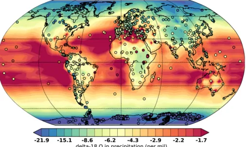
Fig. 1. Annual mean δ18O in precipitation in iLOVECLIM compared to the GNIP database (IAEA, 2006) and Masson-Delmotte et al. (2008) database for Antarctic snow isotopic composition (coloured circles).
(GCMs) have been used exclusively to simulate separately water isotopes in the atmosphere and ocean components. In-deed, given the computational constraints imposed by the use of coupled climate GCMs, it is still useful and insightful to use simpler models to simulate the evolution of water iso-topes millennial timescales. Hence, the development of water isotope tracing in earth system models of intermediate com-plexity (EMIC) has some potential to fill this gap. The limita-tion in the latter class of models is the availability of enough physical mechanisms in the atmosphere modelled to provide a sufficiently realistic representation of water isotopes for our current climate in the first instance. The strongest constraint in that respect is consistent advection or transport of water since the largest spatial signals are due to along-path frac-tionation with the distance to the source of moisture (Craig and Gordon, 1965; Dansgaard, 1964).
This was proven possible in the CLIMBER-2 model that includes a 2.5 dimensional statistical–dynamical atmosphere with full computation for moisture advection (Roche et al., 2004), albeit under the constraint of a simplistic water clo-sure assumption. In the present study, we evaluate the re-sults obtained with the newly developed 18O module for the iLOVECLIM coupled climate model, a derivative of the LOVECLIM model (Goosse et al., 2010). The difficulty does not reside presently in the advection of moisture which is computed explicitly but in the reduction of the atmosphere to three vertical layers, with a single moist layer (Opsteegh et al., 1998), complicating the vertical fractionations along the precipitation path (Roche, 2013).
The equations and verification of implementation was achieved in the first part (Roche, 2013). In the present manuscript, we present a comparison of fully coupled
atmosphere–ocean–vegetation modelling results under pre-industrial conditions with present-day δ18O data for the atmospheric and oceanic component. The performance of iLOVECLIM to sufficiently track the present-day water cycle and its potential for past climate studies will be enlightened. A third study and last part is evaluating the model from the perspective of a model–data integration with late Holocene carbonate data (Caley and Roche, 2013).
2 Simulation set-up
In the following, we present results of a 5000 yr equilib-rium run under fixed pre-industrial boundary conditions that was used already in the first part of this study to verify the implementation of the water isotopic scheme. The atmo-spheric pCO2is chosen to be 280 ppm, methane concentra-tion is 760 ppb and nitrous oxide concentraconcentra-tion is 270 ppb. The orbital configuration is calculated from Berger (1978) with constant year 1950. We use present-day land–sea mask, freshwater routing and interactive vegetation.
With regards to the water isotopes, the atmospheric mois-ture is initialised at −12 ‰ and the ocean at 0 ‰ for δ18O. The consistency of our integration is checked by ensuring that the water isotopes are fully conserved in our coupled system.
3 Results and discussion 3.1 Atmospheric component 3.1.1 Annual mean results
Starting from the annual mean distribution of δ18O in precip-itation (cf. Fig. 1), we obtain a qualitatively good agreement with the Global Network for Isotopes in Precipitation (GNIP) data (IAEA, 2006; Masson-Delmotte et al., 2008). The main gradients (depletion towards drier and colder areas) as well as the land–sea contrasts are globally faithfully reproduced. Our results also capture the lower δ18O value in precipitation in the equatorial regions with respect to the tropical regions (the so-called “equatorial trough”, Craig and Gordon, 1965) that is predicted from the lower E/P ratio that exists in these regions.
Two exceptions may be noted: first, the too low gradient towards low δ18O content in precipitation in northern North America toward the Arctic ocean; second, the overall δ18O content in precipitation for continental eastern Africa that is too low with respect to what is expected from the measure-ments. The latter is due to a displacement of the zone of high tropical precipitations simulated by ECBilt towards the east in comparison to climatology, hence the higher continental fractionation over the continent. Finally, the largest bias that may be noted is the high δ18O content of precipitation over the Mediterranean Sea and the adjacent regions. Since this is also the case for the δ18O of seawater (see below), we in-terpret this mismatch as a consequence as the low resolution of the ocean model and thus inadequate exchange of waters between the Mediterranean and the North Atlantic Ocean. Indeed, as can be seen in Goosse et al. (2010) (their Fig. 4), running CLIO at about 3◦resolution implies the need for a 6◦ latitudinal extent for the Gilbraltar Strait, hence the absence of Spain. This caveat in the model together with the low resolution of the atmospheric model displace the continen-tality effect over Europe and could explain the late appari-tion of the eastern δ18O trends together with much enriched values on the western side of Europe whereas data indicate more depleted values (Fig. 1). Indeed, water evaporated from the Mediterranean Sea is greatly enriched and contributes to higher δ18O across Europe and into Asia (LeGrande and Schmidt, 2006). Nonetheless, although it appears further in-land in the model, the gradient over Europe for the δ18O (reflecting gradual rainout from air masses with decreasing mean annual air temperature and increasing continentality) is represented (Fig. 1), indicating a robust representation of the Rayleigh distillation, as was noted in Roche (2013).
3.1.2 Large-scale climatic to δ18O relationship
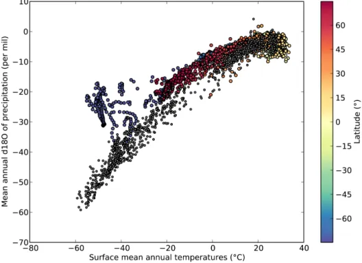
To further test the applicability of the isotopic atmospheric component, we present in Figs. 2 and 4 two classical δ18O to climatic variable relationship: the first compares annual
mean δ18O to annual mean temperature (the well-known Dansgaard relationship, Dansgaard, 1964) and the second the δ18O to annual mean precipitation relationship.
Comparing the values obtained in the model (coloured points) with those from the GNIP dataset (grey dots), we see that the Dansgaard relationship does exist in our model (as already noted in Roche, 2013) albeit with a slightly lower slope. We interpret the lower slope as an underestimation of the fractionation towards lower temperatures/latitudes, orig-inating from the use of the very simplified approximation of a single moist layer for the atmosphere in ECBilt (Roche, 2013). Another factor is the altitudinal effect which char-acterises the decrease in δ18O with height. This production of isotopically depleted precipitation is physically related to the Rayleigh distillation that takes place when an air parcel, lifted uphill, condenses. Taking into account the low resolu-tion of the model that flattens all high elevaresolu-tion topography, we can explain why the δ18O values modelled in Greenland (−20 to −25 ‰) are not sufficiently depleted in comparison with data (−25 to −30 ‰) (Fig. 3). We note as well that the relationship breaks at low temperature over Antarctica, as indicated by their latitude. We have investigated this as-pect in the development and verification step (Roche, 2013) and found that this mismatch is probably due to a numerical issue in the advection–diffusion scheme at very low humid-ity content. We have so far not been able to find a satisfactory solution to deal with this issue and thus keep it as such for the time being.
We have previously computed the linear relationship be-tween temperature and precipitation (Dansgaard, 1964) as the regression between the mean annual temperature and the mean precipitation-weighted δ18O. Assuming that δ18O in precipitation can be used as a proxy for local temper-ature, only temperature at times when precipitation occurs can be recorded in the δ18O signal. A good example of such an issue is given by the use of the Dansgaard relation-ship during the Last Glacial Maximum in Greenland: during this cold period the precipitation was only falling in sum-mer in Greenland, biasing the δ18O-temperature relationship (Werner et al., 2000). Therefore, it appears physically more relevant to calculate the regression between precipitation-weighted temperature and precipitation-precipitation-weighted δ18O. The precipitation-weighted temperature is computed as
T∗(i) =P 1 jP (i, j )
X j
(T (i, j ) P (i, j )) (1)
for a given cell i, where the sum over the j is the sum over the twelve months of the year in our case. The relationship between the obtained T∗and δ18O in precipitation is slightly more linear (cf. Fig. 3) than the classical Dansgaard relation-ship (Fig. 2). Indeed, a linear fit to the modelled weighted relationship obtains a R2value of 0.87 against 0.83 for the standard relationship. In particular, tropical regions are more aligned with the mid-latitudes ones (as shown by the quasi
1496 D. M. Roche and T. Caley: Water isotopes in the iLOVECLIMmodel
Fig. 2. Annual δ18O-temperature relationship in iLOVECLIM compared to the GNIP database (IAEA, 2006) and Masson-Delmotte et al. (2008) database for Antarctic snow isotopic composition. So-called “Dansgaard relationship”. Coloured circles are from iLOVECLIM: their colour indicating latitude and grey dots are the observations.
Fig. 3. δ18O-temperature weighted by precipitation relationship in iLOVECLIM from monthly data (coloured circles, colour indicating latitude).
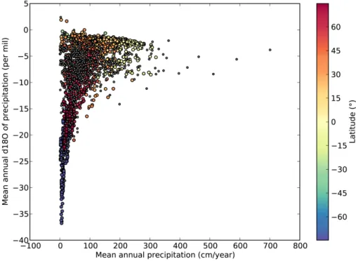
Fig. 4. Annual δ18O-precipitation relationship in iLOVECLIM compared to the GNIP database (IAEA, 2006) and Masson-Delmotte et al. (2008) database for Antarctic snow isotopic composition. So-called “precipitation amount” relationship. Coloured circles are from iLOVECLIM: colour indicating their latitude and grey dots are the observations.
identical R2 value obtained by a second-order polynomial fit, 0.88); same goes for the high latitude regions, apart from Antarctica. For Antarctica (Masson-Delmotte et al., 2008), the spread of anomalous points is still visible, with the possi-bility that the few clustered points around T∗= −40◦C are more or less consistent with the linear model while in general those between −30 and −60◦C are clearly biased.
As tropical regions have a fairly constant temperature over the year and are more driven by the amount of precipitation, it is usual to plot the relation between that amount and the δ18O of precipitation. Model results in the δ18O-precipitation amount space (Fig. 4) is in very good agreement with data showing no relationship at low mean annual precipitation and a positive relationship at high precipitation amount. Our model only fails to reproduce the very few regions with very high precipitation amount, above ' 350 cm per year. The re-sults are nonetheless very good given the simplicity of our atmospheric model.
3.1.3 Results from monthly data
To further evaluate our iLOVECLIM simulation results on a global scale, it is tempting to compare directly the seasonal evolution at specific stations representative of various climate conditions: Reykjavik (northern Atlantic), Vienna (central Europe), Ankara (eastern Mediterranean) and Belem (South America). Since our results are at relatively coarse resolution and since we have some regional biases as described in the annual mean results, we cannot expect to reproduce faithfully
the mean. Hence, results are presented centred around the mean for GNIP stations and for the closest model data point (Fig. 5). While we model the correct seasonal amplitude over the year at each chosen GNIP station, we do not obtain an evolution of δ18O similar to the data at Belem and Reyk-javik, but we do in Vienna and Ankara. As noted before, the two latter regions are areas where the mean annual discrep-ancy is largest between the data and the model (around 10 ‰) whereas the bias is much smaller for Belem and Reykjavik. This reinforces the notion that for a large part of Europe, the annual cycle is simply shifted to heavier values in the model with respect to the data.
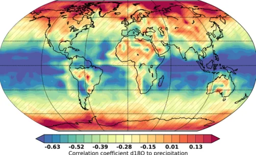
The observed discrepancy between model and data for climate variables (temperature and precipitation) affects our data model comparison for oxygen isotopes. For the tropical region of Belem, we expect a more important control of pre-cipitation on the δ18O signal than temperature that stays rela-tively constant through the year. The abnormal high precipi-tation rate in the model from September to December (Fig. 5) explains probably the more δ18O depleted values that we ob-serve for the same period in our model whereas the data are more enriched. To evaluate whether iLOVECLIM could be used to study the interannual variability of the precipitation in the tropics, we evaluate the correlation of the interannual relationship between monthly anomalies (seasonal cycle sub-tracted) of δ18O in precipitation and temperature and precip-itation rate (Figs. 6 and 7). A negative and significant cor-relation is found in the tropics (−30◦, 30◦) between δ18O
1498 D. M. Roche and T. Caley: Water isotopes in the iLOVECLIMmodel
Fig. 5. Seasonal temperature, precipitation and δ18O evolution in precipitation at specific stations (Belem, Vienna, Reykjavik and Ankara) in iLOVECLIM from monthly data. The blue line is data from the IAEA (IAEA, 2006) and the red line is iLOVECLIM at the corresponding latitude and longitude. All data are normalised around their annual average.
and precipitation rate, mainly over the oceanic regions. On the contrary, for the relationship between δ18O in precipita-tion and temperature, a stronger and significant correlaprecipita-tion is observed at higher latitudes whereas the correlation is in-significant at lower latitudes. Exceptions occur in the north-ern high latitudes where significant negative correlations are observed in Siberia and the North America regions. We con-clude that oxygen isotopes mainly record interannual vari-ability of the precipitation in the tropics. However, in our model, results are not significant for a large part of tropi-cal continents. The validity of these observed relationships at the interannual timescale would be tested by simulating long time periods and past climates such as the Last Glacial Maximum. By comparison, δ18O in precipitation also mainly record interannual variability of the precipitation in the trop-ics in LMD-z v4 GCM (Risi et al., 2010) and previous studies (Hoffmann et al., 2003; Ramirez et al., 2003).
3.2 Oceanic component
3.2.1 Annual mean near-surface δ18O
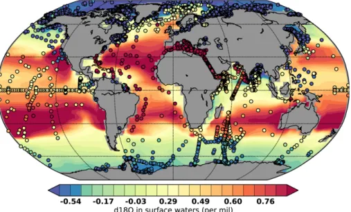
Surface mean ocean δ18O results obtained (Fig. 8) are in very good agreement with data from the GISS database (Schmidt et al., 1999). The latitudinal gradients are faithfully repro-duced with lower δ18O in high latitude regions and higher δ18O in tropical regions. We obtain as expected from data a
lower δ18O around the equator the latter being a less evap-orative region than the tropics, as seen already in the atmo-spheric part. The contrast between the evaporative zones and the mid-latitudes is well represented in the model. We ob-serve nonetheless some notable discrepancies between the modelled distribution and data. One clearly apparent mis-match is the western Indian Ocean where we simulate much lower δ18O in near-surface ocean than observed in reality. This bias is due to a shift of the African precipitation regions from the west to the east of the continent, leading to much less saline waters (and unrealistically depleted δ18O) in the western Indian Ocean. Another region where model and data do not agree is offshore California: the isotopic signal of the North Pacific depleted values does not penetrate as far south as observed. A similar pattern is observed in the GISS model (Schmidt et al., 2007); we do not have an explanation yet for such a disagreement.
Figure 9 shows details of the North Atlantic and the Arc-tic Ocean region. We chose the region because of the strong gradients in δ18O occurring due to the different water masses. Our results show an excellent match between the model re-sults and the near-surface ocean data from the GISS database. In particular, we can clearly follow the δ18O enriched water masses entering the Arctic ocean, mixing with the δ18O de-pleted waters there. The fronts are generally reproduced in the right place. From these results we may infer a too lit-tle influence of Arctic waters in Baffin Bay in our model in
Fig. 6. Spatio-temporal correlation between δ18O in precipitation and precipitation rate within iLOVECLIM. Figure is constructed from monthly mean data. Hatching indicates areas where correlation is poor (<0.35).
Fig. 7. Spatio-temporal correlation between δ18O in precipitation and temperature within iLOVECLIM. Figure is constructed from monthly mean data. Hatching indicates areas where correlation is poor (<0.35).
comparison to the data and a slightly too small western ex-tent for the North Atlantic drift in the Nordic seas, showing the potential for regional scale evaluation of our coupled cli-mate model. The match between the modelled and observed near-surface ocean δ18O is rather good in this critical region where deep water masses are formed that fill the whole North Atlantic.
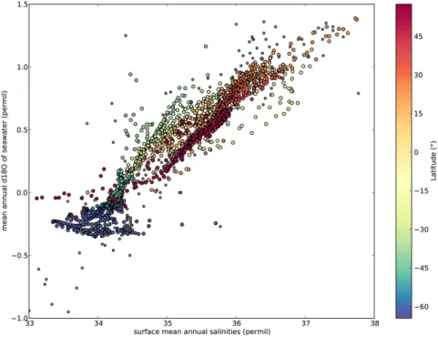
Since surface water δ18O and salinity are affected by very similar processes (evaporation, precipitation, water masses advection and mixing), it is important to ascertain whether the observed δ18O to salinity relationship can be reproduced
in our control simulation. Figure 10 shows that for the At-lantic Ocean, simulated δ18O–salinity is in very good agree-ment with observed data for the same ocean basin for all lat-itudes. We restricted the lower salinity range to 33 ‰ since the GISS database also contains data points with very non-salty conditions, reflecting rivers mouths and not open ocean. Since we are using a relatively coarse grid model, we cannot expect to reproduce such conditions. The obtained modelled gradient for the δ18O-salinity relationship is 0.43 (Roche, 2013), in close accordance with the observed one (0.52),
1500 D. M. Roche and T. Caley: Water isotopes in the iLOVECLIMmodel
Fig. 8. Near-surface ocean δ18O in sea water in iLOVECLIM compared to the GISS database (Schmidt et al., 1999) (coloured circles).
Fig. 9. Same as Fig. 8 but zoomed on the North Atlantic region.
while still bearing the too low fractionation towards high lat-itude, as observed in the atmospheric model.
Regarding the Pacific Ocean near-surface waters (Fig. 11), while we still obtain a fair agreement, modelled data points from the northern tropical latitudes to the north are shifted towards higher δ18O values. This reflects the overestimation of δ18O already seen in Fig. 8 especially in the southern trop-ics. Since the salinities are in good accordance with the data in that particular region it implies that there is an overestima-tion of fracoverestima-tionaoverestima-tion at evaporaoverestima-tion in this region. One likely
source is an underestimation of near-surface ocean humidity since this term is the most effective in the governing equation (Roche, 2013). The notable difference between the northern Pacific and the southern Pacific yield two parallel lines, the northern one being offset half a per mil in δ18O and one per mil in salinity. Though the spread observed is still within the observed data range, further investigation would be needed to fully understand that difference.
3.2.2 Annual mean deep ocean δ18O
Since we obtain satisfactory results at the surface of the oceans it is worth comparing our results to available data for the interior of the oceans. It shall be noted that repre-senting the deep ocean δ18O is complicated since it depends strongly on the δ18O content at the location of deep water formation, a rather restricted area. A relatively small shift in δ18O may lead to a substantial drift in deep ocean δ18O with an opposite drift in surface waters δ18O. The cross sections presented are averaged over all the considered ocean basin, using a mask to define the ocean basins. The data points from the GISS database are all collapsed on the same cross section but not averaged. Thus, certain data points may represent val-ues from specific locations that are not comparable to the mean.
In the Atlantic Ocean (Fig. 13), the simulated δ18O dis-tribution clearly show the mark of the main water masses. From the north, the North Atlantic deep waters (NADW) are marked by higher δ18O content, around 0.2 ‰. NADW ex-tends in our model almost to the bottom of the ocean (as shown in Goosse et al., 2010) where it mixes with the Antarc-tic bottom water (AABW) coming from the south. The latter water mass is marked by low δ18O content. In the South-ern Ocean, the Antarctic intermediate waters are also marked
Fig. 10. Near-surface ocean annual δ18O-salinity relationship in iLOVECLIM (coloured dots) and GISS database (grey dots) (Schmidt et al., 1999) for the Atlantic Ocean. Colour scale indicates the latitude for the iLOVECLIM circles.
Fig. 11. Near-surface ocean annual δ18O-salinity relationship in iLOVECLIM (coloured dots) and GISS database (grey dots) (Schmidt et al., 1999) for the Pacific Ocean. Colour scale indicates the latitude for the iLOVECLIM circles.
by a specific δ18O content around 0 ‰, moving northwards at about 1000 m deep. This general structure is in excellent agreement with the available δ18O observations, both in ver-tical and latitudinal distributions. Very low observed surface values around 60◦N are in coastal areas and hence are not
representative of the zonal mean ocean δ18O. We nonetheless note a discrepancy in the deep ocean (from 3000 m to the bot-tom) where the modelled distribution of δ18O is around 0 ‰ while seawater measurements are around 0.25 ‰, between 20◦S and 30◦N. Since the distribution of the modelled δ18O
1502 D. M. Roche and T. Caley: Water isotopes in the iLOVECLIMmodel
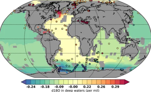
Fig. 12. Mean 2500–3500 m depth δ18O in sea water in iLOVECLIM compared to the GISS database (Schmidt et al., 1999) (coloured circles).
Fig. 13. Atlantic zonal mean for the δ18O of seawater in iLOVECLIM compared to the GISS database (Schmidt et al., 1999) (coloured scale) presented as a latitudinal–depth (m) transect.
field is otherwise in very good agreement with data, we in-fer that this discrepancy may arise from two distinct causes. First, the fact that we compare a zonal average field in the model versus point-based measurements from data tends to smooth the east–west contrasts with a western deep Atlantic having higher δ18O content (by 0.1 to 0.2 ‰) than the eastern deep Atlantic, as shown on Fig. 12. The intrusion of Labrador deep water is particularly prominent in that respect, with val-ues of 0.3 ‰. Second, the fact that even when taking this as-pect into account there is still an underestimation of the δ18O in the model (see in the tropical deep Atlantic on Fig. 12 for example) shows that the influence of NADW with pos-itive δ18O content might not be strong enough in the deep
Fig. 14. Pacific zonal mean for the δ18O of seawater in iLOVECLIM compared to the GISS database (Schmidt et al., 1999) (coloured scale) presented as a latitudinal–depth (m) transect.
North Atlantic. Interestingly, Fig. 12 clearly shows that the southern deep Atlantic is reproduced faithfully in the model. This indicates that the entrance of southern source water in the southern deep Atlantic is correctly represented and is not the cause of the problem mentioned. Whether the cause is not enough northern sourced deep water export to the deep ocean or inadequate mixing of that northern sourced waters in the ocean interior is a matter for investigation.
For the Pacific Ocean, presented in Fig. 14, the results are similar though less clearly visible. We obtain a good agree-ment for the δ18O distribution until 2000 m deep in all the Pacific and reasonable low δ18O content around the Antarctic at all depth. As in the Atlantic, the deep ocean (from 30◦S)
has a too low δ18O content in our simulation by about 0.2 ‰. Again, we can only state that it may be due to incorrect mix-ing in the deep ocean or not enough influence of δ18O rich waters. Closer to the surface, our simulation reproduce faith-fully the vertical and latitudinal gradients. In the North Pa-cific, the data is dominated by the large number of points from the Okhotsk Sea that does not represent the mean of the ocean basin. In addition, we have seen previously that mod-els (iLOVECLIM and GISS) failed to reproduce the North Pacific depleted values in offshore California. Together, this can explain the disagreement between model and data for the North Pacific zonal mean comparison.
4 Conclusions
In the present manuscript, we have evaluated a pre-industrial control run against present-day observation of δ18O in pre-cipitation and in the ocean waters. For the atmospheric part, we found that apart from central Antarctica, our model pro-duces results in good accordance with what is known from the GNIP dataset, with some caveats due to the simplicity of the approach taken. If the general gradients (latitudinal, oceanic to continental) are well reproduced, the trends to-wards colder and drier are generally underestimated, indicat-ing a too low fractionation in our sindicat-ingle moist layer atmo-sphere.
From the ocean perspective, we obtain a very good agree-ment between the simulated δ18O values in the oceans and the observed values as recorded in the GISS database. The slightly too low gradient found in the atmosphere is naturally also present in the oceanic part of our coupled model since the system is coupled and closed with respect to water and isotopic water content.
Overall, with the caveats mentioned above, we obtain a water isotope enabled coupled climate model well suited for long-term simulation of the changing climate. Since our aim is to use the model in palaeoclimatic context, the next logical step is to evaluate the model against available δ18O proxy for the late Holocene. This is the subject of the third part of our study (Caley and Roche, 2013) and will enable us to iden-tify the advantage and caveats of our model in such compar-isons under the well-known conditions of the pre-industrial climate.
Acknowledgements. T. Caley is supported by NWO through the VIDI/AC2ME project no. 864.09.013. D. M. Roche is supported by NWO through the VIDI/AC2ME project no. 864.09.013 and by CNRS-INSU. The authors wish to thank A. Landais for use-ful discussion on isotopic fractionation process and D. Paillard for discussion pertaining to technical developments of the ocean part of the model. Two anonymous reviewers are thanked for useful comments that helped improve the manuscript through the review process. Institut Pierre Simon Laplace is acknowledged for host-ing the iLOVECLIM model code under the LUDUS framework
project (https://forge.ipsl.jussieu.fr/ludus). All figures where pro-duced using the Matplotlib software (Hunter, 2007), whose creators are gratefully acknowledged.
This is NWO/AC2ME contribution number 02. Edited by: R. Marsh
The publication of this article is financed by CNRS-INSU.
References
Berger, A.: Long-term variations of caloric insolation resulting from earths orbital elements, Quaternary Res., 9, 139–167, 1978. Caley, T. and Roche, D. M.: Caley, T. and Roche, D. M.: δ18O
wa-ter isotope in the iLOVECLIM model (version 1.0) – Part 3: A palaeo-perspective based on present-day data–model comparison for oxygen stable isotopes in carbonates, Geosci. Model Dev., 6, 1505–1516, doi:10.5194/gmd-6-1505-2013, 2013.
Craig, H. and Gordon, L.: Deuterium and oxygen 18 variations in the ocean and the marine atmosphere, Consiglio Nazionale delle Ricerche, Laboratorio di Geologia Nuclerne, Pisa, 9–130, 1965. Dansgaard, W.: Stable Isotopes in Precipitation, Tellus, 16, 436–
468, 1964.
Delaygue, G., Jouzel, J., and Dutay, J.-C.: Oxygen 18-Salinity re-lationship simulated by an oceanic general circulation model, Earth Planet. Sci. Lett., 178, 113–123, doi:10.1016/S0012-821X(00)00073-X, 2000.
Goosse, H., Brovkin, V., Fichefet, T., Haarsma, R., Huybrechts, P., Jongma, J., Mouchet, A., Selten, F., Barriat, P.-Y., Campin, J.-M., Deleersnijder, E., Driesschaert, E., Goelzer, H., Janssens, I., Loutre, M.-F., Morales Maqueda, M. A., Opsteegh, T., Mathieu, P.-P., Munhoven, G., Pettersson, E. J., Renssen, H., Roche, D. M., Schaeffer, M., Tartinville, B., Timmermann, A., and Weber, S. L.: Description of the Earth system model of intermediate complex-ity LOVECLIM version 1.2, Geosci. Model Dev., 3, 603–633, doi:10.5194/gmd-3-603-2010, 2010.
Hoffmann, G., Werner, M., and Heimann, M.: Water isotope module of the ECHAM atmospheric general circulation model : A study on timescale from days to several years, J. Geophys. Res., 103, 16871–16896, doi:10.1029/98JD00423, 1998.
Hoffmann, G., Ramirez, E., Taupin, J. D., Francou, B., Ribstein, P., Delmas, R., and D¨urr, H.: Coherent isotope history of Andean ice cores over the last century, Geophys. Res. Lett., 30, 1179, doi:10.1029/2002GL014870, 2003.
Hunter, J. D.: Matplotlib: A 2D graphics environment, Comput. Sci. Eng., 9, 90–95, 2007.
IAEA: Isotope Hydrology Information System, The ISOHIS Database, available at: http://www.iaea.org/water (last access: 8 March 2012), 2006.
Jacobs, S. S., Fairbanks, R. G., and Horibe, Y.: Origin and evo-lution of water masses near the Antarctic continental margin: Evidence from H218O/H216O ratios in seawater, in: Oceanol-ogy of the Antarctic Continental Shelf, edited by: Jacobs, S. S.,
1504 D. M. Roche and T. Caley: Water isotopes in the iLOVECLIMmodel
Antarctic Research Series, 43, 59–85, AGU, Washington, DC, doi:10.1029/AR043, 1985.
Joussaume, S., Jouzel, J., and Sadourny, R.: A general circulation model of water isotope cycles in the atmosphere, Nature, 311, 24–29, 1984.
Jouzel, J., Russell, G. L., Suozzo, R. J., Koster, R. D., White, J. W. C., and Broecker, W. S.: simulations of the hdo and H2 O-18 atmospheric cycles using the nasa giss general-circulation model – the seasonal cycle for present-day conditions, J. Geo-phys. Res., 92, 14739–14760, doi:10.1029/JD092iD12p14739, 1987.
Lee, J.-E., Fung, I., DePaolo, D. J., and Henning, C. C.: Analysis of the global distribution of water isotopes using the NCAR atmo-spheric general circulation model, J. Geophys Res. Atmos., 112, D16306, doi:10.1029/2006JD007657, 2007.
LeGrande, A. N. and Schmidt, G. A.: Global gridded data set of the oxygen isotopic composition in seawater, Geophys. Res. Lett., 33, L12604, doi:10.1029/2006GL026011, 2006.
Masson-Delmotte, V., Hou, S., Ekaykin, A., Jouzel, J., Aristarain, A. J., Bernardo, R. T., Bromwich, D., Cattani, O., Delmotte, M., Falourd, S., Frezzotti, M., Gall´ee, H., Genoni, L., Isaks-son, E., Landais, A., Helsen, M. M., Hoffmann, G., Lopez, J., Morgan, V., Motoyama, H., Noone, D., Oerter, H., Petit, J.-R., Royer, A., Uemura, R., Schmidt, G. A., Schlosser, E., Sim˜oes, J. C., Steig, E. J., Stenni, B., Sti´evenard, M., van den Broeke, M. R., van de Wal, R. S. W., van de Berg, W. J., Vimeux, F., and White, J. W. C.: Database of Antarctic snow isotopic composi-tion,, doi:10.1594/PANGAEA.681697, 2008.
Mathieu, R., Pollard, D., Cole, J. E., White, J. W. C., Webb, R. S., and Thompson, S. L.: Simulation of stable water isotope varia-tions by the GENESIS GCM for modern condivaria-tions, J. Geophys. Res., 107, 4037, doi:10.1029/2001JD900255, 2002.
Noone, D. and Simmonds, I.: Associations between delta O-18 of water and climate parameters in a simulation of atmo-spheric circulation for 1979-95, J. Climate, 15, 3150–3169, doi:10.1175/1520-0442(2002)015<3150:ABOOWA>2.0.CO;2, 2002.
Opsteegh, J., Haarsma, R., Selten, F., and Kattenberg, A.: ECBILT: A dynamic alternative to mixed boundary conditions in ocean models, Tellus, 50, 348–367, available at: http://www.knmi.nl/
∼selten/tellus97.ps.Z, 1998.
¨
Ostlund, H. G. and Hut, G.: Arctic Ocean water mass balance from isotope data, J. Geophys. Res. Ocean., 89, 6373–6381, doi:10.1029/JC089iC04p06373, 1984.
Ramirez, E., Hoffmann, G., Taupin, J. D., Francou, B., Ribstein, P., Caillon, N., Ferron, F. A., Landais, A., Petit, J. R., Pouyaud, B., Schotterer, U., Simoes, J. C., and Stievenard, M.: A new Andean deep ice core from Nevado Illimani (6350 m), Bo-livia, Earth Planet. Sci. Lett., 212, 337–350, doi:10.1016/S0012-821X(03)00240-1, 2003.
Risi, C., Bony, S., Vimeux, F., and Jouzel, J.: Water-stable isotopes in the LMDZ4 general circulation model: Model evaluation for present-day and past climates and applications to climatic in-terpretations of tropical isotopic records, J. Geophys. Res., 115, D12118, doi:10.1029/2009JD013255, 2010.
Roche, D. M.: δ18O water isotope in the iLOVECLIM model (ver-sion 1.0) – Part 1: Implementation and verification, Geosci. Model Dev., 6, 1481–1491, doi:10.5194/gmd-6-1481-2013, 2013.
Roche, D., Paillard, D., Ganopolski, A., and Hoffmann, G.: Oceanic oxygen-18 at the present day and LGM: equilibrium simulations with a coupled climate model of intermediate complexity, Earth Planet. Sci. Lett., 218, 317–330, 2004.
Rozanski, K., Aragu`as-Aragu`as, L., and Gonfiantini, R.: Iso-topic patterns in modern global precipitation, in: Climate Change in Continental Isotopic Records, edited by: Swart, P. K.,Geophysical Monograph Series, 78, 1–36, AGU, Washing-ton DC, doi:10.1029/GM078p0001, 1993.
Schmidt, G. A.: Oxygen-18 variations in a global ocean model, Geophys. Res. Lett., 25, 1201–1204, doi:10.1029/98GL50866, 1998.
Schmidt, G. A., Bigg, G. R., and Rohling, E. J.: Global Seawater Oxygen-18 Database – V1.21, available at: http://www.giss.nasa. gov/data/o18data/, 1999.
Schmidt, G. A., LeGrande, A. N., and Hoffmann, G.: Water iso-tope expressions of intrinsic and forced variability in a cou-pled ocean-atmosphere model, J. Geophys. Res., 112, D10103, doi:10.1029/2006JD007781, 2007.
Tindall, J. C., Valdes, P. J., and Sime, L. C.: Stable water isotopes in HadCM3: Isotopic signature of El Nino Southern Oscillation and the tropical amount effect, J. Geophys. Res., 114, D04111, doi:10.1029/2008JD010825, 2009.
Werner, M., Mikolajewicz, U., Heimann, M., and Hoffmann, G.: Borehole versus isotope temperatures on Greenland: Seasonnal-ity does matter, Geophys. Res. Lett., 27, 723–726, 2000. Werner, M., Langebroek, P. M., Carlsen, T., Herold, M., and
Lohmann, G.: Stable water isotopes in the ECHAM5 gen-eral circulation model: Toward high-resolution isotope model-ing on a global scale, J. Geophys. Res. Atmos., 116, D15109, doi:10.1029/2011JD015681, 2011.
Xu, X., Werner, M., Butzin, M., and Lohmann, G.: Water isotope variations in the global ocean model MPI-OM, Geosci. Model Dev., 5, 809–818, doi:10.5194/gmd-5-809-2012, 2012.
Yoshimura, K., Kanamitsu, M., Noone, D., and Oki, T.: Historical isotope simulation using Reanalysis atmospheric data, J. Geo-phys. Res., 113, D19108, doi:10.1029/2008JD010074, 2008. Zhou, J., Poulsen, C. J., Pollard, D., and White, T. S.: Simulation
of modern and middle Cretaceous marine delta O-18 with an ocean-atmosphere general circulation model, Paleoceanography, 23, PA3223, doi:10.1029/2008PA001596, 2008.