Key aspects of stratospheric tracer modeling

(1)

HAL Id: hal-00301342

https://hal.archives-ouvertes.fr/hal-00301342

Submitted on 6 Jun 2006

HAL is a multi-disciplinary open access

archive for the deposit and dissemination of sci-entific research documents, whether they are pub-lished or not. The documents may come from teaching and research institutions in France or abroad, or from public or private research centers.

L’archive ouverte pluridisciplinaire HAL, est destinée au dépôt et à la diffusion de documents scientifiques de niveau recherche, publiés ou non, émanant des établissements d’enseignement et de recherche français ou étrangers, des laboratoires publics ou privés.

Key aspects of stratospheric tracer modeling

B. Bregman, E. Meijer, R. Scheele

To cite this version:

B. Bregman, E. Meijer, R. Scheele. Key aspects of stratospheric tracer modeling. Atmospheric Chemistry and Physics Discussions, European Geosciences Union, 2006, 6 (3), pp.4375-4414. �hal-00301342�

(2)

ACPD

6, 4375–4414, 2006

Stratospheric tracer modeling key aspects

B. Bregman et al. Title Page Abstract Introduction Conclusions References Tables Figures J I J I Back Close

Full Screen / Esc

Printer-friendly Version Interactive Discussion

EGU

Atmos. Chem. Phys. Discuss., 6, 4375–4414, 2006 www.atmos-chem-phys-discuss.net/6/4375/2006/ © Author(s) 2006. This work is licensed

under a Creative Commons License.

Atmospheric Chemistry and Physics Discussions

Key aspects of stratospheric tracer

modeling

B. Bregman, E. Meijer, and R. Scheele

Royal Netherlands Meteorological Institute, P.O. Box 201, 3730 AE, De Bilt, The Netherlands Received: 3 February 2006 – Accepted: 7 March 2006 – Published: 6 June 2006

(3)

ACPD

6, 4375–4414, 2006

Full Screen / Esc

EGU Abstract

This study describes key aspects of global chemistry-transport models and the impact on stratospheric tracer transport. We concentrate on global models that use assim-ilated winds from numerical weather predictions, but the results also apply to tracer transport in general circulation models. We examined grid resolution, numerical di ffu-5

sion and dispersion of the winds fields, the meteorology update time intervals, update frequency, and time interpolation. For this study we applied the three-dimensional chemistry-transport Tracer Model version 5 (TM5) and a trajectory model and per-formed several diagnoses focusing on different transport regimes. Covering different time and spatial scales, we examined (1) polar vortex dynamics during the Arctic winter, 10

(2) the large-scale stratospheric meridional circulation, and (3) air parcel dispersion in the tropical lower stratosphere. Tracer distributions inside the Arctic polar vortex show considerably worse agreement with observations when the model grid resolution in the polar region is reduced to avoid numerical instability. Using time interpolated winds improve the tracer distributions only marginally. Considerable improvement is found 15

when the update frequency of the assimilated winds is increased from 6 to 3 h, both in the large-scale tracer distribution and the polar regions. It further reduces in particular the vertical dispersion of air parcels in the tropical lower stratosphere. The results in this study demonstrates significant progress in the use of assimilated meteorology in chemistry-transport models, which is important for both short- and long-term integra-20

tions.

1 Introduction

Global three dimensional chemistry transport models (hereafter referred to as CTMs) driven by actual meteorology from numerical weather predictions are crucial for the in-terpretation of many observational data. The great advantage is the direct comparison 25

(4)

trans-ACPD

6, 4375–4414, 2006

Full Screen / Esc

EGU

port. CTMs are thus ideally designed for detailed sensitivity studies of key processes important for climate, which would be computationally too expensive for Chemistry-Climate Models (CCMs). Major areas of interest are the polar regions, owing to the prevailing chemical ozone loss during winter and its sensitivity towards climate change, and the tropical region where the main entrance of air into the stratosphere is located 5

(WMO,2002). The ability of a direct comparison with observations also allows model sensitivity studies to investigate basic model parameters, such as grid resolution and advection schemes, but also the quality of the wind fluxes or vectors and the way the meteorological information is implemented in the CTM.

The impact of grid resolution on the atmospheric composition remains an important 10

subject of discussion. Searle et al. (1998) show that a horizontal resolution of 3◦ is sufficient to calculate polar chemical ozone loss, but Marchand et al. (2003) in con-trast found substantial differences after increasing their model resolution from 2◦×2◦ to 1◦×1◦. Another model study also focused on the effect of spatial resolution in the polar region by evaluating methane distributions (van den Broek et al.,2003). An important 15

outcome was the significant overestimation of methane in the lower stratosphere at the edge and inside the polar vortex. An increase of the horizontal grid resolution to 1◦×1◦gave negligible improvement and thus indicated very small sensitivity to horizon-tal resolution. This results support the conclusions fromSearle et al.(1998), although the conclusions here were based on long-lived tracer distributions. The results in this 20

study however contrasts these findings.

CTMs and CCMs suffer from numerical instability in regions of strong zonal winds and relatively small grid cells. The most critical regions are located at the poles, in particular during the winter, but also in the vicinity of storm tracks. Negative tracer mass can occur when the transport distance during one advection time step exceeds the size 25

of the grid cell, the so-called Courant-Friedrichs-Lewy (CFL) criterion. Commonly, this is avoided by reducing the grid resolution or by averaging the wind vectors or mass fluxes, but its impact on tracer transport has sofar not been investigated.

(5)

ACPD

6, 4375–4414, 2006

Full Screen / Esc

EGU

to excessively small time steps. To overcome this difficulty we introduced an iteration procedure for tracer advection in the TM5 model with locally adjusted time steps (Krol

et al.,2005). InKrol et al.(2005) the focus was on the troposphere. In this study we will demonstrate the dramatic impact on the stratospheric tracer distribution.

The quality of the winds provided by the numerical weather predictions is another 5

factor affecting tracer transport. The winds are subject to data assimilation within the model prediction and are often referred to as Data Assimilation System or DAS winds (Schoeberl et al.,2002). The quality of particularly the stratospheric winds is affected by the presence of spurious variability or “noise”, inherently introduced through the as-similation procedure, either through a lack of suitable observations or by inaccurate 10

treatment of the model biases. This unwanted variability causes enhanced dispersion that accumulates in time. Hence, the impact of dispersion increases with increasing dy-namic time scales. It may therefore not be a serious problem for the troposphere where the dynamic turnover times are relatively short. However, the stratospheric circulation contains much longer time scales where spurious variability in DAS winds becomes 15

very critical. One of the consequences is enhanced dispersion and an enforced large-scale stratospheric meridional circulation, causing tracer residence times to be con-siderably shorter than observed (Schoeberl et al.,2002;Douglass et al.,2003;Meijer

et al.,2004). The most critical region is the tropical lower stratosphere, where the ma-jority of the air enters the stratosphere. Moreover, this is a very complicated region for 20

data assimilation due to a lack of observations and because the atmosphere deviates from geostrophical balance, which complicates proper treatment of model biases.

Meijer et al. (2004) and Scheele et al. (2005) show that the intensity of disper-sion in the DAS winds increases when the assimilation procedure is less accurate or less sophisticated. For example, the ECMWF utilizes three- and four-dimensional 25

assimilation procedures (3DVAR and 4DVAR respectively). 4DVAR is a temporal ex-tension of 3DVAR, and thus more accurate but also computationally more expensive. A comprehensive description of the ECWMF assimilation procedures can be found at

(6)

bal-ACPD

6, 4375–4414, 2006

Full Screen / Esc

EGU

anced winds for each model time step, due to the inclusion of time. Because of compu-tational expenses the long-term re-analyses (ERA40) has been performed with 3DVAR, while the operational data, analyses and forecasts (referred to as “Operational Data” or OD) are produced with 4DVAR. Comparing both data sets thus yields information about the impact of assimilation accuracy on tracer transport. Ozone is a useful tracer, 5

since its distribution is very vulnerable to the strength of large-scale stratospheric circu-lation. Laat et al.(2006) andvan Noije et al. (2004) show a very strong accumulation of ozone in the extra-tropical lower stratosphere when using ERA40 winds, resulting in significant overestimation compared to observations. When applying OD winds, the agreement becomes much better. Indeed, van Noije et al. (2004), Simmons et al.

10

(2005) and Scheele et al. (2005) have shown that OD winds contain less dispersion than ERA40 winds in the tropical lower stratosphere and provide more realistic extra-tropical downward ozone fluxes (van Noije et al.,2004) and more realistic stratospheric residence times (Meijer et al.,2004). However, even with OD the circulation remains too strong (Laat et al.,2006), which has led to the practical decision to constrain strato-15

spheric ozone down to 100 hPa in the extra-tropics with ozone climatology (van Noije

et al.,2004) for the tropospheric multi-year IPCC chemistry-transport runs. However for coupled troposphere-stratosphere runs this solution is undesirable.

Recently, a comprehensive model intercomparison was performed with winds and temperatures from a variety of data assimilation systems, focusing on the 2002 Antarc-20

tic vortex split (Manney et al., 2005). They show substantial differences between the models that apply different DAS, with operational (4DVAR) analysis performing better than re-analysis (3DVAR) data, consistent with the studies described above.

Despite shortcomings in ERA40 winds, the dynamical variability can be simulated quite well (Hadjinicolaou et al.,2005;Chipperfield,2006). This is in line with a compar-25

ison between DAS winds from different numerical weather predictions, where ERA40 winds were found to agree excellent with observed variability (Randel et al.,2003). It is important to note that instantaneous variability and enhanced dispersion or noise in the winds are two separated issues. The above mentioned studies with ERA40 clearly

(7)

ACPD

6, 4375–4414, 2006

Full Screen / Esc

EGU

demonstrate this.

Recently, we have evaluated forecasts instead of analyses, assuming that forecasts are physically more balanced and thus are expected to contain less noisy winds, similar to the differences between 3DVAR and 4DVAR winds. Indeed, in a recent trajectory study we have shown that by increasing the forecast length the dispersion in the tropical 5

lower stratosphere is significantly reduced (Scheele et al.,2005). In line with these results the mean age of air becomes older in the extra-tropical stratosphere, closer to observations (Meijer et al.,2004). However, it now became too old in the tropical lower stratosphere, while still remaining too young in the extra-tropics.

The representation of the large-scale meridional circulation in the stratosphere by 10

DAS winds considerably improves when using isentropic vertical coordinates and heat-ing rates instead of vertical wind velocity or mass fluxes on pressure levels (Mahowald

et al.,2002). Although an isentropic coordinate seems physically more appropriate for stratospheric dynamics, a mass correction needs to be performed in order to balance the divergence with the isentrope tendencies, which will impact the tracer distributions. 15

This is a fundamental mass balance problem that applies to both CTMs and GCMs independent of the vertical coordinate system, as has been demonstrated by J ¨ockel

et al. (2001) and for which different mass fixers have been introduced (cf. Bregman

et al.,2003;Rotman et al.,2004). When integrating over a full vertical range from the upper stratosphere to the surface, the isentropic vertical coordinate needs to be ad-20

justed from purely isentropic to a hybrid of pressure and isentropes. So far only two models have inferred such a hybrid coordinate (Mahowald et al., 2002;Chipperfield,

2006), which still contain mass imbalance issues but are promising developments. By applying the algorithm ofSegers et al.(2002),Bregman et al.(2003) have shown that the use of mass fixers can be avoided by applying mass-flux advection, without 25

violating mass conservation. This is a fundamental underlying aspect in this study. We have demonstrated complete mass conservation using the hybrid sigma-pressure coordinate, while sofar this has not been proven for other vertical coordinate systems.

(8)

ACPD

6, 4375–4414, 2006

Full Screen / Esc

EGU

modeling because of cloud processes, convection and other physical processes which are important for tracer transport. This is one of the major reasons why the majority of the current global models, including CTMs and CCMs use a fixed pressure or a hybrid sigma-pressure coordinate system, without implying that all these physical processes are accurately represented when using a hybrid sigma-pressure coordinate.

5

A fundamental question remains: are we able to perform meaningful multi-year tracer integrations applying DAS winds with a sigma-pressure vertical coordinate? The an-swer depends on the progress in improving DAS wind quality and the way they are applied in global models. Improving the quality of DAS winds is an ongoing activity and progress is being made in filtering techniques and the error covariances and bias cor-10

rections (Polavarapu et al.,2005), Simmons, personal communication). In this study we concentrate on how DAS winds are applied in CTMs.

One aspect not commonly addressed in CTM studies applying DAS winds is the ef-fect of the update time interval on the modeled tracer distributions and the variability within the time interval. Generally the winds are updated every 6 h. However, strato-15

spheric dynamical variability occurs on time scales shorter than 6 h (Shepherd et al.,

2000;Manson et al.,2002), so that a considerable part of real variability is neglected. Additionally, the winds can be assumed constant over this time interval (instantaneous), averaged or interpolated in time. Instantaneous winds introduce discontinuities when changing time interval, leading to spurious variability, while averaging can be regarded 20

as a (strong) wave filter. Examining ERA40 winds,Legras et al. (2005) show that de-creasing the meteorological update time interval from 6 to 3 h reduces spurious motions considerably.

There have only been very few model studies addressing 3-hourly meteorological data in CTMs (Wild et al.,2003;Legras et al.,2005;Berthet et al.,2006). However, a 25

more general evaluation at different spatial scales and including the effect of interpola-tion within the time interval has not yet been performed.

To evaluate all these key aspects for tracer transport we perform a variety of integra-tions, including different model grid resolutions and vertical layers, as well as different

(9)

ACPD

6, 4375–4414, 2006

Full Screen / Esc

EGU

time intervals of the DAS winds, including time averaging and interpolation effects. We use CH₄ as a passive tracer to focus on polar transport in a similar set-up as in

van den Broek et al.(2003). We further apply the age of air diagnose as a first-order approximation of the impact on the large-scale stratospheric meridional circulation and perform trajectory calculations to examine the degree of dispersion in the tropical lower 5

stratosphere in the assimilated winds.

The outline of this paper is as follows. We first briefly describe TM5 and the recent updates. The next section addresses the model sensitivity experiments for the polar region, the general stratospheric circulation and dispersion in the tropical lower strato-sphere, which is followed by a section describing the results. We will show that the 10

model updates as well as the sensitivity experiments have a substantial impact on the tracer distributions. This section is followed by a summary of all comparisons providing guidelines for use of assimilated winds in CTMs.

2 Model description

The global Tracer Model, TM5 is a grid point Eulerian 3-D CTM and is an extended 15

version of the TM3 model. The TM3 model has been used widely in the modeling community (e.g.Dentener et al.,1999;Peters et al.,2001;Houweling et al.,1998;Van

den Broek et al.,2000;Bregman et al.,2001,2002). The original version of the model has been developed by Heimann (1995); Heimann and Keeling (1989). TM5 uses forecasts of the European Centre for Medium-range Weather Forecasts (ECMWF) to 20

drive the transport with a default update time interval of 6 h. It further uses mass fluxes for advection of the tracers as described in van den Broek et al. (2003). The model contains a Cartesian grid and consists of a two-way nested grid zooming over selected areas by increasing the horizontal resolution, currently up to 1◦×1◦. The model further contains hybrid σ-pressure levels with the top level at 0.1 hPa. The representation of 25

the model winds has recently been adjusted to assure mass conservation by (Segers

(10)

ACPD

6, 4375–4414, 2006

Full Screen / Esc

EGU

(Bregman et al.,2003).

An important feature of the TM5 zoom version is the mass consistent two-way nest-ing that allows global studies includnest-ing zoom areas. Because of the grid zoomnest-ing capability the model architecture has changed fundamentally. The model structure and the zooming concept have been described in detail and the model was successfully 5

validated for the lower troposphere byKrol et al.(2005).

A validation of stratospheric tracers was performed byvan den Broek et al.(2003). The TM5 version used in this study differs in some important aspects from the version used by van den Broek et al. In the previous version used by van den Broek et al.

(2003), the advection scheme contained only first-order moments or slopes (Russel

10

and Lerner,1981). This version also uses second-order moments advection (Prather,

1986). Further, the previous version used a fixed number of vertical levels, while this version allows different vertical resolutions. Another important update is the ability to adjust the model advection time step locally when the CFL criterion (i.e., air mass transport exceeding the grid cell in one model advection time step) is violated (Krol

15

et al.,2005). This update avoids a reduction of the polar grid in the polar regions, and thus allows a proper sensitivity study of model grid resolution.

The reduction of the polar grid is necessary because the horizontal grid cell area of a regular model grid decreases towards the poles and even becomes so small that the CFL criterium is violated and negative grid and consequently negative tracer mass 20

would occur. This is particularly relevant for models containing mass-flux advection. To avoid this, without reducing the advection time step too severely, the model grid is artificially reduced. This reduction is established either by merging of the grid cells or the mass fluxes. See Sect. 2.3 in Krol et al. (2005) for a detailed description of the reduced grid treatment in TM5. Invan den Broek et al.(2003) the reduced polar grid is 25

illustrated within the zoom grid in Fig. 1 of that paper.

Up to now the reduction of the polar grid has not be validated because of computa-tional limits, since the advection time steps would not only become excessively small (i.e. a few minutes only), but they would also have to be applied over the whole model

(11)

ACPD

6, 4375–4414, 2006

Full Screen / Esc

EGU

domain. The new advection algorithm allows sufficiently small advection time steps by means of an iteration procedure for the location where a CFL isolation occurs, rather than by applying it over the whole grid. Whenever a CFL violation occurs, the number of iterations is determined by reducing the mass fluxes accordingly until the violation vanishes. Then the advection is performed with the required number of iterations. The 5

iteration was tested for numerical errors by using idealized passive tracers, and the er-rors remained close to machine precision (not shown). This improvement was crucial, because it allows integrations at higher model grid resolutions.

3 Experimental set-up

For the model evaluation in the Arctic region methane was used as a passive tracer and 10

the model was integrated from October 1999 to April 2000. The experimental setup, including the model constraints, are similar as in van den Broek et al. (2003). The reader is referred to this study for more details. We would like to emphasize that this experiment focuses on the high latitudes, since methane is treated as a passive tracer. For this reason the integration period is not more than half a year, but is sufficient 15

for the purpose of this experiment. However, caution must be taken for mid-latitudes in the middle and upper stratosphere where the impact of chemistry becomes more pronounced.

The mean age of air is calculated by applying the “tracer pulse” method, as described inHall and Plumb(1994) andHall et al. (1999). The tracer pulse method consists of 20

an inert tracer released in the troposphere with unity mass mixing ratio by applying a delta-function. The tracer mixing ratios in the stratosphere are a measure of the mean residence time, calculated using the Green function (Hall and Plumb,1994). The year 2000 is integrated repetitively for 20 years. The mean age is calculated as the first moment of the derived spectrum after 20 years.

25

For the trajectory experiment the trajectory model is used as described byScheele

(12)

exam-ACPD

6, 4375–4414, 2006

Full Screen / Esc

EGU

ined the dispersion of air parcels in the tropical lower stratosphere by calculating 50-day back trajectories similar to the experiments performed bySchoeberl et al.(2002). Approximately 10000 trajectories started between 10◦S–10◦N at 460 K potential tem-perature level, corresponding to a pressure of 50 hPa or approximately 20 km altitude. As a measure of dispersion, the fraction of air parcels crossing the 10◦S and 10◦N 5

border before moving through the tropopause is calculated. Figure1shows the setup of the experiment. The tropopause is defined on basis of potential vorticity or temper-ature lapse rate. SeeScheele et al.(2005) for a detailed discussion. In addition to the meteorology used by the CTM, we have applied ERA40 forecasts.

The default setup of TM5 includes a global horizontal resolution of 3×2◦, 45 vertical 10

layers and a second-order moment advection scheme, no reduction of the polar grid resolution and using instantaneous (constant) wind fields updated every 6 h. In addi-tion, a zoom grid with a horizontal resolution of 1×1◦ was applied between 30◦–90◦N, similar as invan den Broek et al.(2003) (see their Fig. 1). All 60 layers of the ECWMF fields have been used, and two subsets with fewer layers: (i) 45 layers, containing all 15

stratospheric and upper tropospheric levels and a reduced number only in the lower troposphere, and (ii) 30 layers, which are obtained by subtracting every second layer from the 60-layer fields. The default number of vertical layers is 45. The results with 45 layers are similar to those using 60-layers (not shown). Two advection schemes were used, a first-order “slopes” scheme (Russel and Lerner,1981) and a second-order mo-20

ments scheme (Prather,1986), with the slopes scheme being most diffusive. Note that with the current model configuration, integrations including a zoom area could only be performed with the first-order advection scheme. The effect of the reduced polar grid was examined in all model configurations. Additional experiments were performed to examine the time discretization. Using the default model setup we used 3-hourly in-25

stead of 6-hourly meteorological data. We further interpolated the winds in time within the update time intervals for both the 6-hourly and the 3-hourly setup to investigate the effect of including wind variability within the meteorological update time interval. The default setup is using 6-hourly instantaneous winds.

(13)

ACPD

6, 4375–4414, 2006

Full Screen / Esc

EGU

A summary of the sensitivity experiments is given in Table 1. Changes to this set are mentioned explicitly in the text.

4 Results

4.1 Horizontal cross sections in the polar region

Horizontal cross sections of CH₄ at 35 hPa have been made for 15 March 2000, af-5

ter integrating the model through the 1999/2000 Arctic winter for five different model versions. This day has been chosen for various reasons. The vortex was still very strong at this stage of the winter so that potential model deficits would be discernible more clearly after accumulation over the whole winter, as was demonstrated in previ-ous model intercomparison (van den Broek et al., 2003). In addition, the late winter 10

vortex becomes subject of considerable dynamic disturbances, providing a useful test for CTMs to capture the dynamic features.

Figure 2 shows the results for the “default”, “red grid”, “1×1” runs with all 6-hourly instantaneous or constant winds, and for the runs with 6-hourly and 3-hourly interpo-lated winds. The methane levels from the reduced grid run are clearly higher with a very 15

weak vortex edge and little tracer variability compared to the fields from the other runs. The “default” and the “1×1” runs yield much stronger vortex edges and more variability and both fields are quite comparable. The vortex edge tracer gradients will be shown in more detail in Figs.7 and 8. The vortex gradients become slightly stronger when using the 6-hourly interpolated wind, and considerably stronger when using 3-hourly 20

interpolated winds. Also outside the vortex the tracer fields are considerably lower in this model version, indicating that applying time interpolation and in particular increas-ing the update frequency affects the tracer distribution on a large (hemispheric) scale.

Berthet et al.(2006) also shows reduction in N₂O, HNO₃ and NO₂ in the mid-latitude middle stratosphere when applying 3-hourly winds.

25

(14)

ACPD

6, 4375–4414, 2006

Full Screen / Esc

EGU

with balloon- and borne vertical profiles inside the polar vortex and with space-borne observations across the vortex edge.

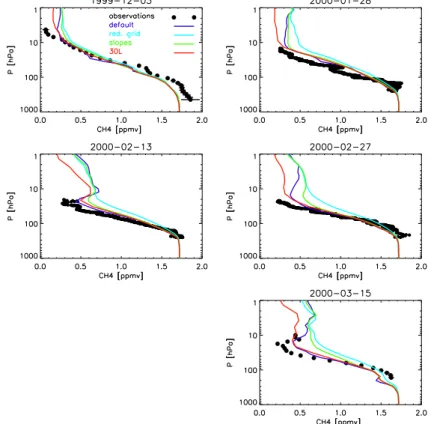
4.2 Comparison with balloon-borne profiles inside the polar vortex

We show a series of figures with comparisons of calculated and observed CH₄profiles for all different model versions. The observations consist of balloon- and space-borne 5

profiles sampled in the polar vortex from December 1999 to April 2000. The selected balloon profiles were all inside the polar vortex and in the study ofvan den Broek et al.

(2003) the largest model underestimation was found for these profiles. The observa-tions were obtained from the balloon-borne Tunable Diode Laser Absorption Spectrom-eter (TDLAS) (Garcelon et al.,2002), the Jet Propulsion Laboratory MkIV interferome-10

ter (Toon et al.,1999), and the space-borne HAlogen Occultation Experiment (HALOE) (Russel-III et al.,1993) on board the UARS satellite. The balloon-borne observations were performed in the frame of the combined projects THird European Stratospheric Experiment on Ozone (THESEO) and Sage III Ozone Loss and Validation Experiment (SOLVE). Seevan den Broek et al.(2003) for more details.

15

Figure 3 shows a comparison with observations for the model versions “de-fault”,“red. grid”, “slopes”, and “30L”. In December the model results are close to the observations. However, the model overestimates CH₄later in the winter and the over-estimation increases in time. Note that the “slopes” results are similar to those pre-sented in van den Broek et al. (2003) and considerably overestimates the observed 20

CH₄ profiles. Another feature is the significant improvement when applying less dif-fusive second-order moments advection. However, the model still overestimates the tracer concentrations. The results from the “red. grid” run are similar to the “slopes” run, but are performed with the second-order moments advection scheme, and reflects the effect of the reduced polar grid. This quite dramatic effect is also visible in Fig.2. 25

This result is quite remarkable, since the reduced grid extends to 70◦N only, while the balloon profiles were located more southwards.

(15)

mes-ACPD

6, 4375–4414, 2006

Full Screen / Esc

EGU

sage to those who apply some kind of grid or mass flux or wind vector merging in the polar region. Another important effect is that a reduction of the polar grid obscures evaluation of grid resolution. To demonstrate this we applied the diffusive first-order slopes advection, as was done invan den Broek et al.(2003) but now with model grid zooming up to the pole (run “1×1”). Figure4 shows that the results improved signifi-5

cantly and are comparable or occasionally even slightly better then the results from the default run with second-order moments advection. This is in contrast with the previ-ous evaluation invan den Broek et al.(2003) where grid zooming did not improve the results and clearly demonstrate the danger of polar grid reduction.

The significant improvement in tracer distribution when increasing the horizontal res-10

olution from 3◦×2◦ to 1◦×1◦ illustrates that model grid resolution is a key issue for the diffusivity of advection. The “1×1” run used the relatively diffusive first-order slopes advection scheme, while the “default” run used much less diffusive second-order mo-ments advection.

The numerical diffusion depends on the amount of tracer information for a given grid 15

cell volume. Figure6shows the tracer information for a 3◦×2◦grid cell in the case of the “default” run (left panel), the “slopes” run (middle panel) and the “1×1” run (right panel). The “default” run contains 10 parameters that determine the tracer level: the first-order slopes (3), the second-order moments (6), and the tracer mass (1). In contrast, the “slopes” run only contains 4 variables with tracer information: the first-order slopes (3) 20

and the tracer mass (1). On the other hand, the zoom region contains 6 more grid cells with each 4 tracer parameters, resulting in a total of 24. The “slopes” run contains the least amount of tracer information and clearly yields the worst results. However, the amount of tracer information in the “1×1” run is twice more than that of the “default” configuration for a 3◦×2◦grid cell, but shows no improvement in the tracer distribution. 25

This may indicate a resolution threshold, which support the findings by Searle et al.

(1998). However, this study demonstrates that such a threshold, if present, depends on the way tracer advection is performed. A diffusive advection scheme clearly overrules the advantage of resolution increase, at least up to 1◦×1◦. It will also depend on the

(16)

ACPD

6, 4375–4414, 2006

Full Screen / Esc

EGU

chemical lifetime of the tracer in question and for a species such as ClO the impact of resolution increase may be substantial (Marchand et al.,2003;Tan et al.,1998).

Next a sensitivity test of vertical resolution was performed. By comparing “default” with “30L” Fig.3shows that the effect of doubling the vertical resolution is restricted to the upper stratosphere (i.e., above the 10 hPa pressure level) where both profiles start 5

to deviate. Due to the limited altitude range of the balloon, no detailed comparison could be performed in the upper stratosphere. Nevertheless, these results indicate that for the current model configuration and experimental setup, vertical resolution does have a significant impact on the tracer distribution, but only in the upper stratosphere.

Finally, we examined the effect of using more wind variability as given by the assim-10

ilated wind fields. Figure5 shows the calculated CH₄ profiles from the “default” run, i.e., with instantaneous 6-hourly wind fields, similar as in Fig.3and6. By interpolating the winds between two subsequent time intervals we account for the wind variability within the model integration time interval. The agreement with observations improves, especially on 15 March 2000. Applying 3-hourly interpolated winds the results are in 15

excellent agreement with the observations.

These results demonstrate the importance to avoid constant winds within the me-teorological time interval and in particular the importance of the update frequency of the DAS winds, which was also shown for mid-latitude tracer profiles inBerthet et al.

(2006). Apparently, more real variability is introduced when applying 3-hourly instead 20

of 6-hourly winds, rather than more “noise”.

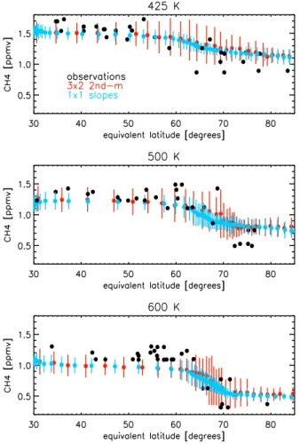
4.3 Comparison with satellite observations: tracer gradient across the vortex edge

Next, we focus on the tracer gradient through the vortex edge. A comparison is per-formed with 15 profiles observed by the HALOE instrument on board the UARS satel-lite. Seevan den Broek et al.(2003) for a more detailed description of these observa-25

tions. These profiles were part of the HALOE sweeps close to the edge of the polar vortex, covering both mid-latitudinal extra- and polar vortex air, and are thus very suit-able to focus on the vortex edge. For such a comparison an equivalent, instead of the

(17)

ACPD

6, 4375–4414, 2006

Full Screen / Esc

EGU

regular Cartesian, latitude coordinate is more useful. Three different potential temper-ature levels have been selected, one close to the polar vortex bottom (425 K), one in the lower stratosphere (500 K) and one in the middle stratosphere (600 K).

Figures7, 8and 9show the results of this comparison for the “default”, “red. grid”, “1×1” runs, “6-hourly-interp” and “3-hourly-interp” experiments. The comparisons are 5

somewhat obscured by the relatively large scatter in the observations, the limited cov-erage in the polar vortex and the modeled variability (denoted by the vertical bar as 1σ). The scatter in the observations is most probably due to the differences in the sampling volume of the observations and the ECWMF potential temperature and po-tential vorticity grid cell volumes. Nevertheless, the latitudinal coverage is sufficient 10

and the tracer gradient across the vortex edge is clearly discernible. As expected, the gradient becomes more pronounced with increasing potential temperature level, both in the observations and in the model results. The default run agrees quite reasonable, while significant underestimation is found for the “red. grid” run, in line with the findings in Fig.3. The tracer gradient at the vortex edge is manifested most clearly in the “1×1” 15

run, although the overall gradient is similar to the default run.

It is interesting that the modeled variability is significantly reduced in the zoom region, especially in active mixing regions: close to the vortex bottom and at the vortex edge. This reflects the increased tracer information in the zoom region, despite the more diffusive advection scheme (see Fig.6).

20

Figure7indicates that the impact of the reduced grid exceeds the polar region. The southern border of the reduced grid in the Arctic is 70◦N, but the differences with the default run extends to 60◦N equivalent latitude. It is remarkable that the impact is found even further south in instantaneous fields. As was demonstrated in Fig. 8 the differences with the zoom region are small with differences up to about 10% and arise 25

at locations where vortex filaments are present.

As can be seen in Fig.9the calculated gradients became stronger when introducing time interpolation and in particular by increasing the meteorological update frequency, in line with the model results described earlier. The differences with the results from the

(18)

ACPD

6, 4375–4414, 2006

Full Screen / Esc

EGU

default run increase with increasing potential temperature level. At 600 K the model un-derestimates the observations at 50–60◦N outside the polar vortex, which is apparent in the results from all model experiments.

Note that even in the best model performance the calculated gradient is slightly un-derestimated, indicating remaining diffusivity and/or the lack of chemistry. Although the 5

effect of chemistry has been tested to have a negligible impact on methane at levels below 10 hPa in a similar model experiment (van Aalst et al., 2004), caution must be taken by treating methane as a passive tracer. Especially close to more chemically active regions of the atmosphere, i.e., the upper stratosphere outside the polar vortex. Indicative for this influence could be the slight underestimation by the model in Figs.8

10

and9at the highest potential temperature level (600 K), which is not present at lower potential temperature levels.

4.4 Age of air experiment

In this experiment we focus on the large-scale meridional circulation in the stratosphere by calculating the mean age of air, as described in the section experimental setup. 15

Here we examine if the earlier found disagreements in calculated and observed mean age of air (Meijer et al., 2004) can be improved by applying 3-hourly DAS winds and time interpolation. We also omitted the reduced polar grid. For the evaluation of the modeled mean age of air we use a compilation of CO₂and SF₆observed on board the ER-2 between 1991–1998 (Andrews et al.,2001), as inMeijer et al.(2004).

20

Figure 10 shows the calculated zonally average mean age of air for three different runs using 6-hourly instantaneous (top panel), 6-hourly interpolated (middle panel) and 3-hourly interpolated winds (bottom panel). The mean age of air is significantly older when using 3-hourly instead of 6-hourly interpolated winds. The effect of interpolation is less significant, although the air becomes 0.5 year older in the upper stratosphere 25

when applying time interpolating in the 6-hourly winds.

Figure11shows the calculated zonally average mean age of air for the same three runs, but now at approximately 20 km altitude, compared to observations. The

(19)

obser-ACPD

6, 4375–4414, 2006

Full Screen / Esc

EGU

vations represent mean age of air derived from airborne in-situ CO₂ measurements on board the ER-2 aircraft in the lower stratosphere (Andrews et al.,2001). The mea-surements are a compilation of all observations between 1991 and 1998. In line with Fig.10 the use of 3-hourly interpolated winds gives the oldest mean age of air. Note that the meridional gradient is significantly steeper than using 6-hourly winds, indica-5

tive of reduced dispersion. Nevertheless the calculated mean age still remains about one year too young in the extra-tropical lower stratosphere. Applying time interpolation in the 6-hourly winds only yields a small improvement. As shown in Fig.10the effect of time interpolation is discernible mainly in the middle and upper stratosphere.

The mean age of air from the 6-hourly instantaneous winds is similar to that calcu-10

lated byMeijer et al.(2004), although they applied a reduced polar grid. This indicates that, in contrast to the findings in the polar study, the reduced polar grid does not affect the stratospheric large-scale tracer transport.

4.5 Back-trajectory experiments

Next we focus on the tropical lower stratosphere, since it is a key region for the large-15

scale meridional circulation. With back-trajectory calculations we calculate the disper-sion of air parcels over 50 days. This time scale is much shorter than the mean age of air, but the dispersion intensity is a useful measure of the noise in DAS winds and thus indirectly relates to the mean age of air (Schoeberl et al.,2002;Scheele et al.,2005). In these calculations we only used interpolated winds. So far we have examined the 20

effect of increasing the update frequency with 4DVAR OD data only. It is interesting to investigate the effect using 3DVAR ERA40 data. We therefore examined three different DAS winds: (1) the default OD 6-hourly winds (red line), similar to the results in Fig. 2 in Scheele et al. (2005). The second and third data set is derived from the 3DVAR ERA40 6-hourly and 3-hourly winds, respectively. Figure12 shows the end points of 25

the air parcels after 50 days. There is considerable scatter, similar to the results from

Schoeberl et al.(2002). As expected, the 6-hourly winds from OD are less dispersive than those from ERA40, as already discussed byScheele et al. (2005). However, the

(20)

ACPD

6, 4375–4414, 2006

Full Screen / Esc

EGU

3-hourly winds from ERA40 show much less vertical dispersion, even compared to the generally less noisy OD winds. Interestingly, the horizontal dispersion is not reduced in the 3-hourly winds.

Figure 13 shows the fraction of air parcels leaving the 10◦S–10◦N latitude band before crossing the tropopause as a measure of dispersion versus the integration time 5

(50 days). In line with Fig.12, the 3DVAR winds (ERA40 6-hourly) show a significant large fraction than the 4DVAR winds (OD 6-hourly). This result is similar as inScheele

et al. (2005). Adding the 3-hourly ERA40 data results in a strong decrease of the fraction. It is even smaller than that calculated with the 6-hourly OD using 4DVAR assimilation.

10

5 Conclusions

In this study we used a CTM (TM5) to investigate the impact of a variety of different model configurations and different representations of the assimilated meteorology on stratospheric tracer transport. In particular we examined the impact of model grid reso-lution, including the reduction of the polar grid, the diffusivity of the advection scheme, 15

and the update frequency and variability in DAS winds. As a diagnose we used CH₄ transport in the Arctic polar vortex and the mean age of air. We further applied a trajectory model to investigate air parcel dispersion in the tropical lower stratosphere.

This study shows that the commonly applied artificial reduction of the polar grid of wind field averaging does have a significant impact on the tracer distribution. The 20

impact well exceeds the area of the reduced grid and these results contain an important message for other studies on polar tracer transport with global models.

The sensitivity experiments show that doubling the vertical resolution substantially affects the tracer distribution in the upper stratosphere, i.e., above 10 hPa, but not below this pressure level. The model results in the upper stratosphere can unfortunately not 25

be evaluated due to a lack of observations.

(21)

ACPD

6, 4375–4414, 2006

Full Screen / Esc

EGU

CH₄distribution in the polar vortex considerably when using first-order (slopes) advec-tion. This is to be expected, since a higher grid resolution represents the vortex edge more realistically. Note that this is only valid without a reduced polar grid. These results are an update of a previous model study where an increase in horizontal grid resolu-tion did not improve the tracer distriburesolu-tions using the same experimental setup. This 5

contrasting result clearly demonstrates the danger of using a reduced polar grid when evaluating model grid resolution. By using adjustable advection time steps, proper high resolution global modeling is feasible in the polar regions.

The impact on stratospheric CH₄ distribution in the polar region by applying more wind variability in the CTM integrations is significant. Using 6-hourly time interpolated 10

instead of instantaneous winds resulted in reduced cross vortex edge mixing and closer agreement with the observed CH₄profiles inside the vortex. Reducing the time interval to 3 h improves the model results even further and yielded excellent agreement with the observed CH₄profiles inside the Arctic vortex.

The stratospheric meridional circulation is examined by diagnosing the mean resi-15

dence time of air in the stratosphere (mean age of air). The mean age of air becomes significantly older in the extra-tropical stratosphere when applying 3-hourly instead of 6-hourly interpolated winds. This indicates that introducing more variability in the wind fields reduces the dispersion. The use of time interpolation is particularly noticeable in the middle and upper stratosphere where the mean age of air becomes 0.5 year older. 20

The tropical mean age of air shows excellent agreement with observations, although the extra-tropical lower stratospheric mean age remains too young with about one year. According to the back-trajectory calculations, the use of 3-hourly winds leads to less vertical dispersion, even with winds produced by the more noisy ERA40 re-analyses winds. It is important to note that the use of 3-hourly winds does not introduce more 25

noise, but more real variability in the wind fields. It remains to be determined what is the most suitable update frequency for stratospheric tracer transport. Such a question is directly related to the representation of the winds from the GCM that provides the winds to the data assimilation system. Waugh et al. (1997) discussed different time

(22)

ACPD

6, 4375–4414, 2006

Full Screen / Esc

EGU

intervals and averaging, however, not for time frequencies of 3 or even less hours. Investigating this problem is however not trivial and is subject of further study.

For models using vertical hybrid sigma-pressure coordinates recent new insights in the use of DAS winds in CTMs has improved the stratospheric tracer representation considerably, both in the polar region as on the large scale. It is recommended not to 5

use a reduction of the polar grid (either through grid cell merging or by wind averag-ing). We also recommend to apply time interpolation instead of using instantaneous winds. In line with the findings from Legras et al. (2005) it is also recommended to apply 3-hourly instead of the commonly used 6-hourly update interval. These results in combination with improvements in data assimilation procedures give new perspectives 10

for long-term tracer integrations.

Acknowledgements. Part of this work is funded by the European Commission, through the project TOwards the Prediction of stratospheric OZone (TOPOZ) III, under contract no. EVK2-CT-2001-00102, the project Stratospheric-Climate Links with Emphasis on the Upper Tropo-sphere and Lower StratoTropo-sphere (SCOUT), and the National (Netherlands) User Support Pro-15

gramme (GO)2. We thank M. Krol and A. Segers for computational support and useful discus-sions.

References

Andrews, A., Boering, K., Daube, B., Wofsy, S., Loewenstein, M., Jost, H., Podolske, J., Web-ster, C., Herman, R., Scott, D., Flesh, G., Moyer, E., Elkins, J., Dutton, G., Hurst, D., Moore, 20

F., Ray, E., Romanshkin, P., and Strahan, S.: Mean ages of stratospheric air derived from in situ observations of CO2, CH4, and N2O, J. Geophys. Res., 106, 32 295–32 314, 2001.

4391,4392,4412

Berthet, G., Huret, N., Lef ´evre, F., Moreau, G., Robert, C., Chartier, M., Pomathiod, L., Pirre, M., and Catoire, V.: On the ability of chemical transport models to simulate the vertical 25

structure of the N₂O, NO₂and HNO₃species in the mid-latitude stratosphere, Atmos. Chem. Phys., 6, 1599–1609, 2006. 4381,4386,4389

(23)

ACPD

6, 4375–4414, 2006

Full Screen / Esc

EGU

Bregman, A., Krol, M., Teyss `edre, H., Norton, W., Chipperfield, M., Pitari, G., Sundet, J., and Lelieveld, J.: Chemistry-transport model comparison with ozone observations in the midlati-tude lowermost stratosphere, J. Geophys. Res., 106, 17 479–17 496, 2001. 4382

Bregman, A., Wang, P.-H., and Lelieveld, J.: Chemical ozone loss in the tropopause region on subvisible ice clouds, calculated with a chemistry-transport model, J. Geophys. Res., 107, 5

doi:10.1029/2001JD000761, 2002. 4382

Bregman, B., Segers, A., Krol, M., Meijer, E., and van Velthoven, P.: On the use of mass-conserving wind fields in chemistry-transport models, Atmos. Chem. Phys., 3, 447–457, 2003. 4380,4383

Chipperfield, M.: New version of the TOMCAT/SLIMCAT off-line chemical transport model: 10

Intercomparison of stratospheric tracer experiments, Q. J. R. Meteorol. Soc., in press, 2006. 4379,4380

Dentener, F., Feichter, J., and Jeuken, A.: Simulation of the transport of Rn222 using on-line and off-line global models at different horizontal resolutions: A detailed comparison with measurements, Tellus, 51, 573–602, 1999. 4382

15

Douglass, A., Schoeberl, M. R., Rood, R. B., and Pawson, S.: Evaluation of transport in the lower tropical stratosphere in a global chemistry and transport model, J. Geophys. Res., 108, 4259, doi:10.1029/2002JD002696, 2003. 4378

Garcelon, S., Gardiner, T., Hansford, G., Harris, N., Howieson, I., Jones, R., McIntyre, J., Pyle, J., Robinson, J., Swann, N., and Woods, P.: Investigation of CH₄and CFC-11 vertical 20

profiels in the Arctic vortex during the SOLVE/THESEO 2000 campaign, in: Proceedings of the general Assembly, Nice, European Geophyisical Society, 2002. 4387

Hadjinicolaou, P., Pyle, J. A, and Harris, N. R. P.: The recent turnaround in stratospheric ozone over northern middle latitudes: A dynamical modeling perspective, Geophys. Res. Lett., 32, L12821, doi:10.1029/2005GL022476, 2005. 4379

25

Hall, T. and Plumb, R.: Age as a diagnostic of stratospheric transport, J. Geophys. Res., 99, 1059–1070, 1994. 4384

Hall, T., Waugh, D., Boering, K., and Plumb, R.: Evaluation of transport in stratospheric models, J. Geophys. Res., 104, 18 815–18 839, 1999. 4384

Heimann, M.: The Global Atmospheric Tracer Model TM2, Tech. Rep. 10, DRKZ-Hamburg, 30

1995. 4382

Heimann, M. and Keeling, C.: A three-dimensional model of atmospheric CO₂transport based on observed winds: 2: Model description and simulated tracer experiments, Geophys. Mon.,

(24)

ACPD

6, 4375–4414, 2006

Full Screen / Esc

EGU

55, 237–275, 1989. 4382

Houweling, S., Dentener, F., and Lelieveld, J.: The impact of non-methane hydrocarbon com-pounds on tropospheric photochemistry, J. Geophys. Res., 103, 10 673–10 696, 1998. 4382 J ¨ockel, P., von Kuhlmann, R., Lawrence, M., Steil, B., Brenninkmeijer, C., Crutzen, P., Rasch, P., and Eaton, B.: On a fundamental problem in implementing flux-form advection schemes 5

for tracer transport in 3-dimensional general circulation and chemistry transport models, Q. J. R. Meteorol. Soc., 127, 1035–1052, 2001. 4380

Krol, M., Houweling, S., Bregman, B., van den Broek, M., Segers, A., van Velthoven, P., Peters, W., Dentener, F., and Bergamaschi, P.: TM5, a global two-way nested chemistry transport zoom model: algorithm and applications, Atmos. Chem. Phys., 5, 417–432, 2005. 4378, 10

4383

Laat, A., Landgraf, J., Aben, I., Hasekamp, O., and Bregman, B.: Assimilated winds for global modelling: evaluation with space- and balloon-borne ozone observations, J. Geophys. Res., in press, 2006. 4379

Legras, B., Pisso, I., Berthet, G., and Lef ´evre, F.: Variability of the Lagrangian turbulent diffusion 15

in the lower stratosphere, Atmos. Chem. Phys., 5, 1605–1622, 2005. 4381,4395

Mahowald, N. M., Plumb, R. A., Rasch, P. J., del Corral, J., Sassi, F., and Heres, W.: Strato-spheric transport in a three-dimensional isentropic coordinate model, J. Geophys. Res., 107(D15), 4254, doi:10.1029/2001JD001313, 2002. 4380

Manney, G., Allen, D., Kr ¨uger, K., Naujokat, B., Santee, M., Sabutis, J., Pawson, S., Swinbank, 20

R., Randall, C., Simmons, A. J., and Long, G.: Diagnosic comparison of meteorological analyses during the 2002 Antarctic winter, J. Atmos. Sci., 133, 1261–1278, 2005. 4379 Manson, A., Meek, C., Koshyk, J., Franke, S., Fritts, D., Riggin, D., Hall, C., Hocking, W.,

MacDougall, J., Igarashi, K., and Vincent, R.: Gravity wave activity and dynamical effects in the middle atmosphere (60–90 km): observations from an MF/MLT radar network, and 25

results from the Canadian Middle Atmosphere Model (CMAM), J. Atmos. Solar-Terr. Phys., 64, 65–90, 2002. 4381

Marchand, M., Godin, S., Hauchecorne, A., Lef ´evre, F., and Chipperfield, M.: Influ-ence of polar ozone loss on northern midlatitude regions estimated by a high-resolution chemistry transport model during winter 1999/2000, J. Geophys. Res., 108, 8326, 30

doi:10.1029/2001JD000906, 2003. 4377,4389

Meijer, E. W., Bregman, B., Segers, A., and van Velthoven, P. F. J.: The influence of data as-similation on the age of air calculated with a global chemistry-transport model using ECMWF

(25)

ACPD

6, 4375–4414, 2006

Full Screen / Esc

EGU

winds, Geophys. Res. Lett., 31, L23114, doi:10.1029/2004GL021158, 2004. 4378, 4379, 4380,4391,4392

Peters, W., Krol, M. C., Dentener, F. J., and Lelieveld, J.: Identification of an El Ni ˜no-Southern Oscillation signal in a multiyear global simulation of tropospheric ozone, J. Geophys. Res., 106, 10 389–10 402, 2001. 4382

5

Polavarapu, S., Ren, S., Rochon, Y., Sankey, D., Ek, N., Koshyk, J., and Tarasick, D.: Data assimilation with the Canadian Middle Atmosphere Model, Appl. Opt., 43, 77–100, 2005. 4381

Prather, M.: Numerical advection by conservation of second-order moments, J. Geophys. Res., 91, 6671–6681, 1986. 4383,4385

10

Randel, W., Fleming, E., Geller, M., Gelman, M., Hamilton, K., Karoly, D., Ortland, D., Pawson, S., Swinbank, R., Udelhofen, P., Wu, F., Baldwin, M., Chanin, M.-L., Keckhut, P., Simmons, A., and Wu, D.: The SPARC intercomparison of Middle Atmosphere Climatologies, Tech. Rep. 20, SPARC newsletter, 2003. 4379

Rotman, D., Atherton, C., Bergmann, D., Cameron-Smith, P., Chuang, C., Connell, P., Dignon, 15

J., Franz, A., Grant, K., Kinnison, D., Molenkamp, C., Proctor, D., and Tannahill, J.: IMPACT, the LLNL 3-D global atmospheric chemical transport model for the combined troposphere and stratosphere: Model description and analysis of ozone and other trace gases, J. Geo-phys. Res., 109, D04303, doi:10.1029/2002JD003155, 2004. 4380

Russel, G. and Lerner, J.: A new finite-differencing scheme for the tracer transport equation, J. 20

Appl. Meteorol., 20, 1483–1498, 1981. 4383,4385

Russel-III, J., Gordley, L., Park, J., Drayson, S., Hesketh, D., Cicerone, R., Tuck, A., Frederick, J., Harries, J., and Crutzen, P.: The Halogen Occultation Experiment, J. Geophys. Res., 98, 10 777–10 797, 1993. 4387

Scheele, R., Siegmund, P., and van Velthoven, P.: Stratospheric age of air computed with 25

trajectories based on various 3-D-Var and 4-D-Var data sets, Atmos. Chem. Phys., 5, 1–7, 2005. 4378,4379,4380,4384,4385,4392,4393

Schoeberl, M., Douglass, A., Zhu, Z., and Pawson, S.: A comparison of the lower stratospheric age-spectra, derived from a General Circulation Model and two data assimilation systems., J. Geophys. Res., 108, 4113, doi:10.1029/2002JD002652, 2002. 4378,4385,4392

30

Searle, K., Chipperfield, M., Bekkie, S., and Pyle, J.: The impact of spatial averaging on calcu-lated polar ozone loss, 1, Model experiments, J. Geophys. Res., 103, 25 397–25 408, 1998. 4377,4388

(26)

ACPD

6, 4375–4414, 2006

Full Screen / Esc

EGU

Segers, A., van Velthoven, P., Bregman, B., and Krol, M.: On the computation of mass fluxes for Eulerian transport models from spectral meteorological fields, in: Proceedings of the 2002 International Conference on Computational Science, Lecture Notes in Computer Science (LNCS), Springer Verlag, 2002. 4380,4382

Shepherd, T., Koshyk, J., and Ngan, K.: On the nature of large-scale mixing in the stratosphere 5

and mesosphere, J. Geophys. Res., 105, 12 433–12 446, 2000. 4381

Simmons, A., Hortal, M., Kelly, G., McNally, A., Untch, A., and Uppala, S.: ECMWF analyses and forecasts of stratospheric winter polar vortex breakup: September 2002 in the Southern Hemisphere and related events, J. Atmos. Sci., 62, 668–689, 2005. 4379

Tan, D., Haynes, P. H., MacKenzie, A. R., and Pyle, J. A.: Effects of fluid-dynamical stirring 10

and mixing on the deactivation of stratospheric chlorine, J. Geophys. Res., 103, 1585–1606, 1998. 4389

Toon, G., Blavier, J.-F., Sen, B., Margitan, J., Webster, C., May, R., Fahey, D., Gao, R., Negro, L. D., Proffit, M., Elkins, J., Romashkin, P., Hurst, D., Oltmans, S., Atlas, E., Schauffler, S., Flocke, F., Bui, T., Stimpfle, R., Boone, G., Voss, P., and Cohen, R.: Comparison of MkIV 15

balloon and ER-2 aircraft measurements of atmospheric trace gases, J. Geophys. Res., 104, 26 779–26 790, 1999. 4387

van Aalst, M., van den Broek, M., Bregman, A., Br ¨uhl, C., Steil, B., Toon, G., Garcelon, S., Hansford, G., Jones, R., Gardiner, T., Roelofs, G., Lelieveld, J., and Crutzen, P.: Tracer transport in the 1999/2000 Arctic polar vortex comparison of nudged GCM runs with obser-20

vations, Atmos. Chem. Phys., 4, 81–93, 2004. 4391

Van den Broek, M., Bregman, A., and Lelieveld, J.: Model study of stratospheric chlorine and ozone loss during the 1996/1997 winter, J. Geophys. Res., 105, 28 961–28 977, 2000. 4382 van den Broek, M., van Aalst, M., Bregman, A., Krol, M., Lelieveld, J., Toon, G., Garcelon, S., Hansford, G., Jones, R., and Gardiner, T.: The impact of model grid zooming on tracer 25

transport in the 1999/2000 Arctic polar vortex, Atmos. Chem. Phys., 3, 1833–1847, 2003. 4377,4382,4383,4384,4385,4386,4387,4388,4389

van Noije, T. P. C., Eskes, H. J., van Weele, M., and van Velthoven, P. F. J.: Implications of the enhanced Brewer-Dobson circulation in European Centre for Medium-Range Weather Forecasts reanalysis ERA-40 for the stratosphere-troposphere exchange of ozone in global 30

chemistry transport models, J. Geophys. Res., 109, D19308, doi:10.1029/2004JD004586, 2004. 4379

(27)

ACPD

6, 4375–4414, 2006

Full Screen / Esc

EGU

Daube, B. C., Elkins, J. W., Fahey, D. W., Dutton, G. S., and Volk, C. M.: Three-dimensional simulations of long-lived tracers using winds from MACCM2, J. Geophys. Res., 102(D17), 21 493–21 514, 1997. 4394

Wild, O., Sundet, J. K., Prather, M. J., Isaksen, I. S. A., Akimoto, H., Browell, E. V., and Oltmans, S. J.: Chemical transport model ozone simulations for spring 2001 over the western Pacific: 5

Comparisons with TRACE-P lidar, ozonesondes and Total Ozone Mapping Spectrometer columns, J. Geophys. Res., 108(D21), 8826, doi:10.1029/2002JD003283, 2003. 4381 WMO: Scientific Assessment of Ozone Depletion, Tech. Rep. 47, WMO, 2002. 4377

(28)

ACPD

6, 4375–4414, 2006

Full Screen / Esc

EGU Table 1. A summary of the model experiments. See text for more details for each experiment.

Experiment advection resolution vertical layers winds

“default” or “3×2” 2nd moments 3◦×2◦ 45 6-hourly instantaneous “red. grid” 2nd moments 3◦×2◦ 45 6-hourly instantaneous

“slopes” 1st moments 3◦×2◦ 45 6-hourly instantaneous

“30L” 2nd moments 3◦×2◦ 30 6-hourly instantaneous

“1×1” 1st moments 1◦×1◦ 45 6-hourly instantaneous

“6-hrly interp.” 2nd moments 3◦×2◦ 45 6-hourly time interpolated “3-hrly interp.” 2nd moments 3◦×2◦ 45 3-hourly time interpolated

(29)

ACPD

6, 4375–4414, 2006

Full Screen / Esc

EGU

12 Bram Bregman: STRATOSPHERIC TRACER MODELING KEY ASPECTS

Fig. 1. A schematic view of the trajectory experimental setup. See

text for more details.

Atmos. Chem. Phys., 0000, 0001–24, 2006

www.atmos-chem-phys.org/0000/0001/

Fig. 1. A schematic view of the trajectory experimental setup. See text for more details.

(30)

ACPD

6, 4375–4414, 2006

Full Screen / Esc

EGU

Bram Bregman: STRATOSPHERIC TRACER MODELING KEY ASPECTS 13

Fig. 2. Horizontal cross sections of methane mixing ratios (ppmv) at

35 hPa, 15 March 2000, 0 GMT for the ’default’, ’reduced grid’ and ’1x1’ runs with 6-hourly instantaneous (constant) winds, and with the default configuration busing 6-hourly and 3-hourly interpolated winds.

www.atmos-chem-phys.org/0000/0001/ Atmos. Chem. Phys., 0000, 0001–24, 2006

Fig. 2. Horizontal cross sections of methane mixing ratios (ppmv) at 35 hPa, 15 March 2000,

00:00 GMT for the “default”, “reduced grid” and “1×1” runs with 6-hourly instantaneous (con-stant) winds, and with the default configuration busing 6-hourly and 3-hourly interpolated winds.

(31)

ACPD

6, 4375–4414, 2006

Full Screen / Esc

EGU 14 Bram Bregman: STRATOSPHERIC TRACER MODELING KEY ASPECTS

Fig. 3. Methane profiles (ppmv) versus pressure (hPa), observed

(black dots), and calculated by the model (solid lines) at March 15, 2000. The horizontal bars denote the 2-σ observational uncertainty. Different model versions were used: ’default’ (blue), ’red. grid’ (light blue) ’slopes’ (green) is the default model setup but with a first-order advection scheme. ’30L’ (red) represents a twice as coarse vertical resolution in the stratosphere compared to ’default’.

Fig. 3. Methane profiles (ppmv) versus pressure (hPa), observed (black dots), and calculated

by the model (solid lines) at 15 March 2000. The horizontal bars denote the 2-σ observa-tional uncertainty. Different model versions were used: “default” (blue), “red. grid” (light blue) “slopes” (green) is the default model setup but with a first-order advection scheme. “30L” (red) represents a twice as coarse vertical resolution in the stratosphere compared to “default”.

(32)

ACPD

6, 4375–4414, 2006

Full Screen / Esc

EGU

Fig. 4. As figure 3, but with the results from the default (blue) and ’1x1’ (red) runs. Day 2000-02-27 has been omitted.

Fig. 4. As Fig.3, but with the results from the default (blue) and “1×1” (red) runs. Day

2000-02-27 has been omitted.

(33)

ACPD

6, 4375–4414, 2006

Full Screen / Esc

EGU

16 Bram Bregman: STRATOSPHERIC TRACER MODELING KEY ASPECTS

Fig. 5. As figure 3, but with the results from the default run (blue), using 6-hourly interpolated (green) and 3-hourly interpolated (red) winds. Day 2000-02-27 has been omitted.

Fig. 5. As Fig.3, but with the results from the default run (blue), using 6-hourly interpolated (green) and 3-hourly interpolated (red) winds. Day 2000-02-27 has been omitted.

(34)

ACPD

6, 4375–4414, 2006

Full Screen / Esc

EGU

m rxm, rym, rzm rxxm, rxym, rxzm ryym, ryzm, rzzm m rxm, rym, rzm m rxm rym rzm m rxm rym rzm m rxm rym rzm m rxm rym rzm m rxm rym rzm m rxm rym rzm

'default' 30_x20 _{'slopes' 3}0_x20 _{'slopes' 1}0_x10

Fig. 6. A schematic view of the tracer information per grid cell of

3◦_x2◦_{, when applying second-moments (left) and first-order}

advec-tion without grid zooming (middle) and with grid zooming (right).

Fig. 6. A schematic view of the tracer information per grid cell of 3◦×2◦, when applying second-moments (left) and first-order advection without grid zooming (middle) and with grid zooming (right).