HAL Id: hal-00316287
https://hal.archives-ouvertes.fr/hal-00316287
Submitted on 1 Jan 1996
HAL is a multi-disciplinary open access
archive for the deposit and dissemination of sci-entific research documents, whether they are pub-lished or not. The documents may come from teaching and research institutions in France or abroad, or from public or private research centers.
L’archive ouverte pluridisciplinaire HAL, est destinée au dépôt et à la diffusion de documents scientifiques de niveau recherche, publiés ou non, émanant des établissements d’enseignement et de recherche français ou étrangers, des laboratoires publics ou privés.
First experiences of full-profile analysis with GUISDAP
M. S. Lehtinen, A. Huuskonen, J. Pirttilä
To cite this version:
M. S. Lehtinen, A. Huuskonen, J. Pirttilä. First experiences of full-profile analysis with GUISDAP. Annales Geophysicae, European Geosciences Union, 1996, 14 (12), pp.1487-1495. �hal-00316287�
Ann. Geophysicae 14, 1487—1495 (1996) ( EGS — Springer-Verlag 1996
First experiences of full-profile analysis with GUISDAP
M. S. Lehtinen1, A. Huuskonen2, J. Pirttila¨3
1 Geophysical Observatory, Sodankyla¨, FIN-99600, Sodankyla¨, Finland
2 Finnish Meterological Institute, Geophysical Research, P.O. Box 503, FIN-00101, Helsinki, Finland 3 University of Oulu, Department of Physical Sciences, FIN-90570, Oulu, Finland
Received: 1 March 1996/Revised: 13 June 1996/Accepted: 14 June 1996
Abstract. In this paper we summarize the theory behind full-profile analysis of IS measurements and report first practical experiences with the GUISDAP (Grand Unified Incoherent Scatter Design and Analysis Package) system designed to perform full-profile analysis of any IS measurements efficiently. By fitting whole plasma para-meter profiles over the ionosphere, instead of point values of the parameters supposed to be approximately constant over small range intervals, full-profile analysis is free of underlying assumptions about the slow variation of the plasma parameters as a function of range. We define full-profile analysis as a mathematical inversion problem formalism and explain how it differs from the traditional gated analysis. Moreover, we study the bias introduced to traditional analysis results using realistic model iono-spheres. By applying the full-profile method to data gener-ated from the model ionospheres, we demonstrate that full-profile analysis is free from this kind of bias. Lastly, an example of analysis of real data by full-profile and gated analyses is shown.
1 Introduction
Traditionally, incoherent scatter analysis has been based on the concept of range-gates, where the methods used rely on assumptions about slow spatial variation of the target as a function of scattering point: usually the spatial distribution of the response from the target comes from a relatively small volume in space, being limited both by the antenna beamforms and by the transmitter pulse forms used. This is true for any particular crossed product of the detected radar signal. Consequently, if a set of crossed products with different lag values can be found so that they all correspond to a small enough volume in
Correspondence to: M. S. Lehtinen
space ("a range gate), the most straightforward way to analyze the plasma parameters is to suppose that the plasma stays constant in all of the region having influence on the set of measurements considered. One then fits the plasma parameters by least-squares methods to the chosen measured ACF (autocorrelation function) values using known theories about forms of plasma spectra. The effects of transmitted pulse forms and post-detection filters are then accounted for in various ways by different ‘corrections’ to the signal strengths in the ACF lag estimates.
The assumptions about the slow variation of the plasma as a function of location can be relaxed by modeling the spatial behavior of the plasma and by trying to estimate the spatial behavior of the plasma from the measurements. The estimation problem becomes more complicated this way — the unknown quantities are the plasma parameters defined as functions in three-dimen-sional space instead of single values corresponding to a chosen point in space. Moreover, it becomes necessary to use all measured crossed products simultaneously in the fits and the estimation problem grows from an inverse problem with a few unknowns and may be 6—30 measure-ments (usually the number of measured lag values at each range gate) to a much larger problem, where the unknown is an element in a function space and all the measurements (this could be 103—104 or even more) are handled at the same time.
In this paper we study the situation where the iono-sphere is modeled by one-dimensional unknown-para-meter profiles. These profiles could be understood to be functions of either range or height. This assumption is necessary to make the inversion problem not too ill-behaved — the task of finding an arbitrary function defined in three-dimensional space on the basis of information gathered from a narrow radar beam would clearly be totally impossible.
We will proceed as follows: first we discuss the tradi-tional gated analysis as an inversion problem. Next we show how the full-profile situation is formally defined as an inversion problem and show the methods to solve it
numerically. The crucial parts here involve both the com-puting solutions to the manipulation of the complex con-cept of the incoherent-scatter measurement in a general way as data structures as well as the methods of statistical inversion theory. The modeling of parameter profiles calls for rather complicated ways of interpolation of the pro-files, calculated spectra and ambiguity functions to a hier-archy of grids of various densities.
We base the discussion on several previous papers. The theory of ambiguity functions was originally derived in Lehtinen (1986) and is shown in fullest detail in Lehtinen and Huuskonen (1996). The statistical inversion theory as used here is described in Vallinkoski (1988) and Vallin-koski and Lehtinen (1990b). The theory to approximate the errors due to the fact that the ionosphere is not constant in the region that contributes to the measure-ments (effects of mixing errors), is outlined in Vallinkoski and Lehtinen (1990a). Moreover, we refer to the papers Lehtinen and Huuskonen (1996) and Huuskonen and Lehtinen (1996) on the questions relating to estimation of measurement fluctuations in the general case, also taking care of the situation of a high SNR.
Full-profile analysis has been first reported in Holt et
al. (1992) where full two-dimensional ambiguities were
used in analysis of lag profiles of long-pulse data.
2 IS analysis as a statistical inversion problem A statistical inversion problem is often written as
m"f (x)#e (1)
(see Vallinkoski, 1988; Vallinkoski and Lehtinen, 1990b). Here x is the unknown variable, m is the measurement, and f is the theory mapping describing the relationship of our measurement values to the sought-for unknown vari-able. The random errors of the measurement are ac-counted for by an additional error terme. This notation has some implicit meanings, summarized in the following:
x is a random variable defined in some measurable space,
which in practical numerical studies is usually just Rn. It has a priori distribution density Dpr(x).We suppose in the following that the error term e is Gaussian, independent of x and has covariance matrixR. The conditional density of the measurements m (given x) is then given by
D(mDx)+exp (!12(m!f(x))TR~1(m!f(x))). (2) In statistical inverse problems we are interested in the a posteriori distribution, which is the conditional distribu-tion of the unknown, supposing certain measurement values m have been recorded. This conditional distribu-tion is given simply, apart from normalizadistribu-tion, by fixing
m in the joint probability density and studying it as
a function of x:
D(xDm)+D(m, x)
+
Dpr(x) exp(!12(m!f(x))T R~1(m!f(x))). (3)
2.1 The unknown in gated analysis
In gated analysis, the unknowns we fit are just plasma parameters at a particular height (or a height interval called a range gate, where the parameters are supposed to be constant). Thus, the vector x could be defined by
x"(Ne, ¹i, ¹e/¹i, l, v, . . .). (4) Depending on the height of the range gate under study, the set of variables fitted may look different. For example, it is not necessary to consider collision frequencies at higher altitudes and one can often suppose that ¹e/¹i"1 at lower altitudes.
2.2 The measurements in gated analysis
The measurement m is a subset of the correlator result memory values. It is usually chosen so that the different values in
m"(m1, . . . , mN) (5)
correspond to different lag values of the ACF estimates from the particular range gate. ("the corresponding range ambiguity functions have their masses inside that height interval).
Each measurement point is the complex cross product of two sampled signal values mi"z(ti)z(t@i) or sum of sampled signal products
mi" +
(t,t@)|rgi
z(t) z(t@), (6)
as determined by the correlator algorithm.
2.3 The theory function in gated analysis
The theory function represents the theoretical way of calculating estimates of correlator cross products m, sup-posing that the unknown parameters x"(Ne, ¹i, ¹e/¹i, l, v, . . .) at a particular range gate are known. It consists of two parts:
1) Calculation of theoretical spectra at a suitably chosen sequence of pointsui in frequency axis
Si"S(ui; x)"S(ui; Ne, ¹i,¹e/¹i, l, v, . . .). (7) 2) Calculation of the theoretical ACF estimates mi from these theoretically calculated spectra. This is most effectively done by the spectral ambiguity functions (see Lehtinen and Huuskonen, 1996) that are precalculated for all correlator cross products (or their sums) and for a chosen vector of frequenciesui. Thus, for each mj in the range gate under study we have a spectral ambiguity function ¼j so that
SmjT"¼j·S"+ i ¼ji
S(ui). (8)
The fully expanded formula for the direct theory then becomes
f (x)j"+
i ¼ji
S(ui; x), (9)
with x"(Ne, ¹i, ¹e/¹i, l, v, . . .) our unknown. 3 Full-profile analysis as an inverse problem, simplified case
In the following we formalize the full-profile analysis as a concrete inverse problem. In essence, this means defining different grids and interpolation methods for the different parameters and describing the numerical algorithm for interpolation of the parameters to denser grid points used for spectral calculations and even denser grids used for ambiguity calculations. However, we first formalize a simple version of the idea. This may help the reader to grasp the rather complicated actual imple-mentation.
In full-profile analysis the variable vector x, given by Eq. 4 is replaced by a much longer vector giving the plasma variables at ionospheric-height grid points. The vector can be constructed from the elements of the follow-ing matrix:
xplasma"
A
Ne(r1) ¹i(r1) ¹e(r1)/¹i(r1) l(r1) . . . Ne(r2) ¹i(r2) ¹e(r2)/¹i(r2) l(r2) . . .F F F F F
Ne(rN) ¹i(rN) ¹e(rN)/¹i(rN) l(rN) . . .
B
. (10)
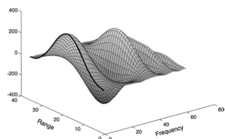
The plasma theory is the same as that used in the gated analysis. The only difference here is that the plasma theory has to be applied to all the parameter set values different spectrum grid points. We need to calculate the two-dimensional spectrum matrix (see Fig. 1)
Sij"S(ui; Ne(rj), ¹e(rj), . . .). (11) Let us denote an arbitrary result memory location by
mk. The dependence of the result memory location on the
Fig. 1. An example of a two-dimensional spectrum
Fig. 2. An example of a two-dimensional ambiguity function
plasma parameters of the whole profile can then be cal-culated by
SmkT"+ i,j
¼kijSij(xplasma), (12) where the ambiguity functions ¼k are two-dimensional spectral ambiguity functions that depend on both fre-quency (index i) and height (index j ); see Fig. 2.
4 Full-profile analysis, actual implementation
The formulation above is in principle useful for full-profile analysis, but it is not the most efficient way to model the full-profile case. The basic reason is that in order for the model to be accurate enough, the density of the range grid must be very high — it needs to be high enough to be able to approximate the fine details of the ambiguity functions. Because the data sampling density is usually approxim-ately the same as the width of the ambiguity functions (at least in typical high-resolution multipulse or alternating-code experiments), it follows that the unknowns are de-fined more densely than the data are gathered. From this it follows that there are more unknowns in the problem than there are data.
It is not impossible to handle this kind of inverse problem — it just calls for a proper use of regularization or a priori information in such a way that the details of the unknown functions are forced not to be smaller than the spatial resolution of the measurements themselves. How-ever, this is rather costly in terms of computational-power requirements and it will be useful to develop more efficient ways of modeling the situation.
In the above solution, spectra have to be calculated on a rather dense grid, and because this is a slow process, we need some faster ways of calculating the full-profile direct theory. The actual, effective solution is therefore much more complicated than the straightforward idea above.
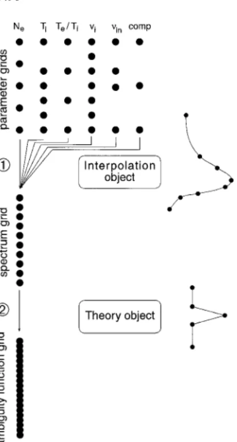
The effective solution to the modeling of the full-profile case is based on a hierarchy of grids and interpolation methods between them. The grids we use are defined in the following (see Fig. 3):
1) Parameter grids: For each plasma parameter, a grid is defined, on whose nodes the plasma parameter values are
Fig. 3. Illustration of the different grids used in full-profile modeling of the ionosphere
defined. Different plasma parameters can have different grids. These grids need generally to be coarser than the spatial resolution of the code itself (roughly speaking: coarser than the width of the ambiguity functions and also coarser than the sample interval of the signals).
2) Spectrum-calculation grid: This grid is finer than the parameter grids. Each parameter is interpolated to this grid, so that interpolated parameter values are available on each point of the grid. Theoretical spectra can then be calculated at each range of the grid.
3) Ambiguity-function grid: This is the grid where ambi-guity functions are represented. It is denser than the spec-trum grid and dense enough to represent the smallest details of the two-dimensional ambiguity-function range dependence.
4.1 The unknowns of actual full profile
Let us denote the parameter-grid range values of the
ith parameters by (rij)Npgi
j/1and the corresponding values of the parameters themselves at the nodes by (pij)Nj/1pgi . Then we can write the unknown of our full-profile inversion problem as x"( p11,p12,p13, . . . p1Npg Ç . . . p21,p22,p23,p24,p25, . . . p2Npg È . . . F pN1, pN2, . . . pNNpgN), (13) where Npg
i is the number of nodes in the parameter grid of the ith parameter. (Note that parameter node values pij as well as the grid-point range values rij are indexed collec-tions of real numbers, but not really matrices, because different parameters could be represented by a different number of grid points, and thus the ‘rows’ of these ‘matrices’ would be of unequal lengths.)
4.2 Parameter-gridPspectrum-grid interpolation
There are three alternatives to this interpolation: a) linear interpolation, b) four-point Lagrange interpolation and c) cubic spline interpolation between the grid point values. The two main interpolation methods here are (a) and (b). Cubic spline interpolation is included essentially as an alternative to the four-point Lagrange interpolation for the cases where an alternative method is necessary to avoid the ‘inverse crime’ situation — a situation where simulated data would be generated using same grids and interpolations as are used in the analysis of it.
The spectral grid range values are now denoted by (rSk)Nsg
k/1and the corresponding interpolated parameter values are denoted by (pik)Nsg
k/1. Linear interpolation is then simply defined by:
pik"(1!h)pij#hpij`1, (14) supposing rij4rSk(rij`1 and h"(rSk!rij)/(rij`1!rij).
In linear interpolation, any interpolated point depends only on the nodes immediately above and below the interpolated points. This results in important savings in calculating derivatives of the direct theory in the fitting procedure.
Lagrange four-point interpolation is defined by
pi"pij~1 (r!rij)(r!rij`1)(r!rij`2) (rij~1!rij)(rij~1!rij`1)(rij~1!rij`2) #pij (r!rij~1)(r!rij`1)(r!rij`2) (rij!rij~1)(rij!rij`1)(rij!rij`2) #pij`1 (r!rij~1)(r!rij)(r!rij`2) (rij~1!rij~1)(rij`1!rij)(rij`1!rij`2) #pij`2 (r!rij~1)(r!rij)(r!rij`1) (rij~2!rij~1)(rij`2!rij)(rij`2!rij`1), (15) supposing r"rSk obeys rij4r(rij`1 (this means that for each range value, we choose four grid nodes for the inter-polation so that two grid-point heights are below the wanted height and two are above it).
Lagrange interpolation is local: each interpolated value depends only on the values of two nodes higher and two nodes lower than the range of the interpolated value. While Lagrange interpolation defined this way does not have exactly the same continuity properties as spline in-terpolation, it behaves much like that in an approximative sense: the derivatives are not continuous over the nodes, but their jumps are very small anyway. This fact, and the simple analytical formula for the Lagrange interpolant make it a useful tool in developing interpolating methods.
When using Lagrange interpolation for range values which do not have two nodes below and above them, we use the four highest or lowest nodes in the interpolation formula anyway. This way we can interpolate the para-meter values over the whole parapara-meter grid and also extrapolate them outside that grid.
Spline interpolation is defined as a specified degree piecewise polynomial going through the specified nodes and having maximal continuity properties that makes the determination of the piecewise polynomial unique and possible. Splines are not local approximations: changing one node value generally changes the spline everywhere. Routines for calculating splines exist in many numerical libraries, which makes them easy to implement. Also, locality is preserved by use of the coefficients of base splines instead of the node values.
4.3 Spectrum calculations
Using whatever interpolation mode between parameter grid and spectrum grid, we arrive at plasma parameter values at each of spectrum grid ranges. The next step in the full-profile direct theory is then to calculate the two-dimensional spectrum at the spectral grid resolution;
Sik"S(ui; (p1k, . . . , pNpk )). (16) The spectral calculations are the most time-consuming part in the whole direct-theory chain. In optimizing analy-sis time the number of spectra should be minimized, meaning that the spectral grid should be as coarse as possible.
Moreover, local interpolation methods save lots of spectral calculations in analysis loops: if changing a single parameter node value changes the interpolated parameter profile only locally, it is not necessary to calculate changed spectra at all spectral grid points when calculating numer-ical estimates to derivatives of the direct theory in the fitting loop.
4.4 From spectra to correlator dump values
The two-dimensional theoretical spectrum is calculated using the range resolution defined by the spectrum grid. However, the ambiguity functions are calculated at a denser grid, and to be able to calculate the two-dimen-sional integrals of the products of the ambiguity functions and the spectra (both functions of range and frequency), the calculated spectra are linearly interpolated to the ambiguity grid (actually the spectra are not interpolated at all — instead linear coefficients between spectral grid points and correlator memory points are calculated and stored. These linear coefficients are equivalent to linear interpolation of the spectra to the ambiguity grid followed by integration over range and frequency).
Linear interpolation is used here exclusively. The reasoning behind this is that in cases where this would not be accurate enough, one can always define the spec-trum grid to be denser and this improves the overall accuracy.
In terms of formulas we do the following: let us deno-te the spectral grid points by rSk and the ambiguity grid points by rW
j . We then suppose we have spectrum values calculated at the spectral grid Sik"S(ui; pi(rSk)) and ambiguity functions at the ambiguity grid ¼ij"¼K(ui;
rW
j ). For programing purposes, linear interpolation from the spectrum grid to other ranges r is most easily defined by using the base splines for linear interpolation, or ‘tri-angle functions’ Bk(r) defined to be the unique piecewise linear functions with
Bk(rSk)"1
Bk(rSn)"0 if nOk (17)
(that is: Bk(r) is a triangle with peak at rSk, sloping down to zero at the adjacent spectral grid points). Then the spectra
Sik are interpolated to an arbitrary range r simply by Si(r)"+
k Bk(r)Sik.
(18) Equation 46 of Lehtinen and Huuskonen (1996) giving the average of the signal cross products as an integral over space and frequency of the product of the spectral ambi-guity function and location-dependent spectra is then evaluated as Sz(t)z(t@)T/R"+ i +j ¼ij +k Bk(rWj)Sik (19) "+ i +k CikSik, (20) where Cik"+
j¼ijBk(rWj) are precalculated coefficients giving the linear relationships between spectra expressed at the spectrum grid and a particular signal lagged prod-uct estimate.
In an actual experiment, many such lagged product estimates may be summed on top of each other in any result memory location. In this case we simply use the corresponding sum of the coefficients Cik to get the linear relationship of the correlator result memory and the spectra at the spectrum grid.
One should note that because the range extents of the ambiguity functions are limited, the coefficients Cik are typically zero for most k. Thus, to be able to calculate the direct theory, we need to store only the nonzero parts of
Cik for any result memory location. This is the final trick
leading to savings in both memory requirements and calculation time. This approach would actually allow for other than linear interpolations to be used between spec-trum grid and ambiguity grid with no penalty in process-ing time.
4.5 Summary of the direct-theory calculation
Because all the details above may seem more complicated than they actually are — they have been developed that way to make the actual numerics as fast as possible — it may be helpful to repeat the steps necessary in direct-theory calculation. We also discuss here the derivative calculations necessary in the fitting loop.
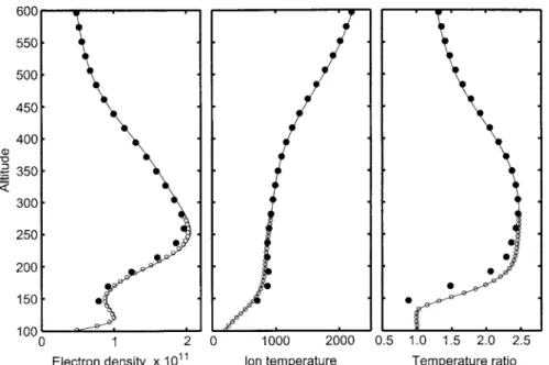
Fig. 4. Results from the gated analysis of long-pulse ( full circles) and alternating-code data (open circles). The model profiles of Ne, ¹i, and ¹e/¹i are given by thesolid line
So, this is how it goes: the starting point is the vector of the unknowns, which are all the plasma parameter values at all of the different parameter grid points (Eq. 13). Each parameter is then interpolated by Eq. 15 to the spectrum grid rSk. Now we can calculate the theoretical spectra Sik at each of the spectrum grid ranges rSk. The theoretical value for each result memory point is finally obtained by using the stored coefficients through Eq. 20.
In the fitting loop we need the partial derivatives of the direct theory with respect to the unknowns. Numerical approximations of these are calculated by changing the value of each of the unknowns at a time, calculating new result memory values and taking the differences of these with the original ones. Because the change of a single plasma parameter value only changes its interpolated values up to two nodes above and two nodes below the changed node (for four-point Lagrange interpolation), we only need to recalculate those spectra whose range values coincide in this interval. This leads to great savings in the analysis time.
5 Bias of gated analysis
The direct theory developed for the full-profile analysis gives us a tool to calculate full IS data dumps for model ionospheres. It is only necessary to define the parameter grid with values of plasma parameters at each grid point. In the following, we will use plasma parameter values based on the model by Alcayde´ et al. (1994). The profiles of Ne, ¹i, and ¹e/¹i are shown by the solid lines in Fig. 4.
If the simulated dumps are then analyzed using the gated-analysis method, we can compare the analysis re-sults with the input model values and thus are able to estimate the bias in the gated analysis. Figure 4 shows gated-analysis results from a EISCAT Common Program experiment (CP-1-K), which uses both alternating-code
and long-pulse modulations. The spectra were calculated at 6-ls (900-m) steps. Thus the spectral grid is finer than the width of the range ambiguity functions for the alter-nating codes (+3 km) and long pulses (+50 km). The ambiguity functions have a 1-ls resolution.
The alternating-code results (open circles) follow close-ly the model parameter profiles. As the range ambiguity function is only 3 km in width, the assumption of small changes is valid within the scattering volume.
The long-pulse results are clearly biased, on the other hand. The electron densities are underestimated around the F-region peak; the ion temperature is overestimated below the F-region peak and underestimated above, whereas the bias in the temperature ratio is opposite. The maximum error is 10% in the electron density and ion temperature and 35% in the temperature ratio. Similar results were obtained by Lathuillere et al. (1986), who also found that the electron temperature, which corresponds to our temperature ratio, was always biased as in Fig. 4, but that the bias in the ion temperature could be either posit-ive or negatposit-ive, depending on the form of the electron density profile. Another case is shown in Holt et al. (1992), where a very long pulse (640ls) combined with a sharp F layer resulted in a clear bias in the electron density.
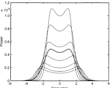
The electron density bias at the F-region peak is straightforward to understand, but interdependencies of the other parameters with each other through the plasma formula can make the explanation of other biases difficult. Moreover, the plasma theory is nonlinear, which causes the smallest ¹e/¹i values by gated analysis to be smaller than any ¹e/¹i values in our model ionosphere. A qualitat-ive explanation is shown in Fig. 5, which shows a set of spectra contributing to the lowest long-pulse gate. The width of the spectrum varies by a factor of two, and thus the average spectrum is very different from the shape of any genuine IS spectrum. When this spectrum, or the corresponding ACF in fact, is analyzed by standard methods, the fit must be poor. Due to the highly nonlinear 1492 M. S. Lehtinen et al.: First experiences of full-profile analysis with GUISDAP
Fig. 6. Analysis results based on the alternating-code (open circles) and long-pulse (full circles) modulations. The data is measured on 16 February 1993, at 1110—1140 UT by the EISCAT UHF radar Fig. 5. Incoherent-scatter spectrum for altitudes 115, 125, 135, 145,
155, 165, and 175 km (thin lines) and the average of the spectra (thick
line). The frequency is given in scaled units
nature of the problem, the results need not be close to the averages of the plasma parameters within the scattering volume.
Figure 6 shows that similar behavior is easily found from experimental data as well. The data was measured on 16 February 1993 at 1110—1140 UT. As the alternat-ing-code results can be assumed to represent the true parameter profiles, the ¹i is overestimated and ¹e/¹i underestimated by the long-pulse analysis, in accordance with the model analysis presented here.
6 Full-profile-analysis results
Figure 7 shows full-profile-analysis results for the same simulated data as used in Fig. 4. The spectral grid point
separation for the fitting is 3 km, which is coarser than the spectral grid used in creating the dump (900 m). In order to avoid the ‘inversion crime’ it is important that simulated data is created with a better accuracy than that used in the analysis. The same parameter grid is used for all parameters fitted (Ne, ¹i, ¹e/¹i, and vi), although the software allows a separate grid for each parameter. Other parameters (lin and ion composition), as well as ¹e/¹i below 110 km, are fixed to model values. The parameter grid point separation is 6 km below 150-km altitude, 12 km below 200 km, and 36 km or 24 km above.
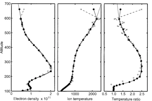
Figure 7 demonstrates how the full-profile method is able to circumvent the problems faced by the gated-analy-sis method. It is easily seen that both full-profile results follow closely the model parameter profiles below the F-region peak where the gated analysis gave a consider-able bias. The most evident deviations are seen at the F-region peak, where both Ne and ¹e/¹i overshoot and ¹i oscillates slightly. The overshoot is caused by the coarse-ness of the parameter grid at this point.
In the topside the 36-km profile behaves smoothly, whereas the profile with 24-km range resolution shows a clear sawtooth structure. This demonstrates that full profile is not able to reach the nominal range resolution of the gated analysis (22.5 km) but instead the best usable resolution is around 30 km for the experiment in question. For completely noiseless data this would not be the case, but our data has a small amount of random noise added. The problems start to arise when the grid spacing is made smaller than half of the length of the ambiguity functions (defined as the half-power width) or if spacing is close to the range separation of successive gates. In the case of the CP-1-K long-pulse measurements, the length of the range ambiguity function is about 60—70 km, which tells that grid spacing at about 35 km or coarser should be useful. The gated analysis treats successive range gates separa-tely, although the spacing (22.5 km) is much less than the range extent of the measurement. Therefore smooth profiles are possible, but the good altitude resolution
Fig. 7. Full-profile analysis results of simulated data. The parameter grid spacing is 6 km below the 150-km altitude, 12 km up to the 200-km altitude, and either 36 km ( full
circles, solid line) or 24 km (crossed, dashed line) above the 200-km altitude. The model
parameter profiles are given by the thin solid
line and the gated-analysis results of the
long-pulse data by the open circle
Fig. 8. Full-profile-analysis results ( full
circles) of EISCAT UHF data measured on 16
February 1993, at 1110—1140 UT. The parameter grid spacing is 6 km below the 150-km altitude, 12 km up to the 200-km altitude, and 30 km above the 200-km altitude. The gated-analysis results of the long-pulse data by the open circles achieved is an illusion. The correlation of the neighboring
gates has not been revealed by the analysis. The full-profile method takes into account the dependence of neighboring points and creates a more realistic figure of the situation.
7 Full-profile analysis of real data
Figure 8 shows finally full-profile-analysis results of the data used in Fig. 6. Analysis is carried out as for the simulated data except that the analysis resolution is 30 km above 200 km. Although slightly noisier than those in Fig. 6, the results show the same features in detail. Thus the full-profile analysis gives a method to analyze
long-pulse data without systematic biases below the F-region peak.
8 Conclusions
We have described a general system designed for using two-dimensional ambiguity functions in connection with functionally modeled ionospheric parameters to fit pro-files of plasma parameters to incoherent-scatter measure-ments. In achieving this goal it has been necessary to develop a hierarchy of different grids and interpolation methods to minimize the calculation task to be feasible in practise. Moreover, special methods of programing and program design are necessary to manage all the complex aspects of a general incoherent-scatter measurement. 1494 M. S. Lehtinen et al.: First experiences of full-profile analysis with GUISDAP
By employing the tools developed we have shown that traditional ways of analysis introduce bias in the results, due to the fact that in the traditional gated-analysis con-cept the variation of the parameters as a function of range is actually forgotten. Using the machinery developed it is possible to simulate actual correlator dumps with the range variation of the parameters taken into account. By applying gated-analysis methods to these dumps and comparing to the original models, the bias can be seen. The existence of this bias has been known previously, but now we have ways to analyze its size numerically.
We have also seen that full-profile analysis is free from this bias and we have shown that the analysis works in practise for both simulated and real data.
Full-profile analysis has been reported previously, but our system is the first one capable of analysis of general measurements, carrying out all calculations automatically on the basis of a general experiment specification. More-over, much effort has been made to minimize the calcu-lation burden by developing the calcucalcu-lations to allow only such resolutions as are necessary at different points in the experiment direct theory calculation.
In the examples of this paper we have used same grid for all parameters, but different grids can easily be used by the system. Future developments will include more gen-eral functional models for the parameters (like, for example, an exponential formula for collision frequency), in addition to the presently possible interpolated models.
Acknowledgements. We are indebted to the Director and staff of
EISCAT for operating the facility and supplying the data. EISCAT is an International Association supported by the research councils of
Finland (SA), France (CNRS), the Federal Republic of Germany (MPG), Norway (NFR), Sweden (NFR) and the United Kingdom (PPARC).
Topical Editor D. Alcayde´ thanks J. Holt and W. Kofman for their help in evaluating this paper.
References
Alcayde´, D., P-L. Blelly, and J. Lilensten, GIVEME, ‘‘General Iono-sphere Visualization and Extraction from a Model for the Eiscat Svalbard Radar’’, Eiscat ¹echnical Note, 94/52, EISCAT Scient-ific Association, Kiruna, Sweden, 1994.
Holt, J. M., D. A. Rhoda, D. Tetenbaum, and A. P. van Eyken, Optimal analysis of incoherent scatter data, Radio Sci., 27, 435—447, 1992.
Huuskonen, A., and M. S. Lehtinen, The accuracy of incoherent scatter experiments: Error estimates valid for high signal levels,
J. Atmos. ¹err. Phys., 58, 453—463, 1996.
Lathuillere, C., W. Kofman, and B. Pibaret, Incoherent Scatter Measurements in the F1-region, J. Atmos. ¹err. Phys., 48, 857—866, 1986.
Lehtinen, M., Statistical theory of incoherent scatter radar measure-ments, Ph.D. thesis, 97 pp., Univ. of Helsinki, Helsinki, Finland,
EISCA¹ ¹echnical Note, 86/45, EISCAT Scientific Association,
Kiruna, Sweden, 1986.
Lehtinen, M. S., and A. Huuskonen, General incoherent scatter analysis and GUISDAP, J. Atmos. ¹err. Phys., 58, 435—452, 1996.
Vallinkoski, M., Statistics of incoherent scatter multiparameter fits,
J. Atmos. ¹err. Phys., 50, 839—851, 1988.
Vallinkoski, M., and M. S. Lehtinen, Parameter mixing errors within a measuring volume with applications to incoherent scatter,
J. Atmos. ¹err. Phys., 52, 665—674, 1990a.
Vallinkoski, M., and M. S. Lehtinen, The effect of a priori knowledge on parameter estimation errors with applications to incoherent scatter, J. Atmos. ¹err. Phys., 52, 675—685, 1990b.