HAL Id: hal-03202398
https://hal.archives-ouvertes.fr/hal-03202398
Submitted on 19 Apr 2021
HAL is a multi-disciplinary open access
archive for the deposit and dissemination of
sci-entific research documents, whether they are
pub-lished or not. The documents may come from
L’archive ouverte pluridisciplinaire HAL, est
destinée au dépôt et à la diffusion de documents
scientifiques de niveau recherche, publiés ou non,
émanant des établissements d’enseignement et de
Taming Past LTL and Flat Counter Systems
Stéphane Demri, Amit Kumar Dhar, Arnaud Sangnier
To cite this version:
Stéphane Demri, Amit Kumar Dhar, Arnaud Sangnier. Taming Past LTL and Flat Counter Systems.
6th International Joint Conference, IJCAR 2012, Bernhard Gramlich; Dale Miller; Uli Sattler, Jun
2012, Manchester, United Kingdom. pp.179-193, �10.1007/978-3-642-31365-3_16�. �hal-03202398�
Taming Past LTL and Flat Counter Systems
?Stéphane Demri1, Amit Kumar Dhar2, and Arnaud Sangnier2
1
LSV, CNRS, ENS Cachan, INRIA, France
2 LIAFA, Univ Paris Diderot, Sorbonne Paris Cité, CNRS, France
Abstract. Reachability and LTL model-checking problems for flat coun-ter systems are known to be decidable but whereas the reachability prob-lem can be shown in NP, the best known complexity upper bound for the latter problem is made of a tower of several exponentials. Herein, we show that the problem is only NP-complete even if LTL admits past-time op-erators and arithmetical constraints on counters. Actually, the NP upper bound is shown by adequately combining a new stuttering theorem for Past LTL and the property of small integer solutions for quantifier-free Presburger formulae. Other complexity results are proved, for instance for restricted classes of flat counter systems.
1
Introduction
Flat counter systems. Counter systems are finite-state automata equipped with program variables (counters) interpreted over non-negative integers. They are used in many places like, broadcast protocols [9] and programs with pointers [12] to quote a few examples. But, alongwith their large scope of usability, many problems on general counter systems are known to be undecidable. Indeed, this computational model can simulate Turing machines. Decidability of reachability problems or model-checking problems based on temporal logics, can be regained by considering subclasses of counter systems, see e.g. [14]. An important and natural class of counter systems, in which various practical cases of infinite-state systems (e.g. broadcast protocols [11]) can be modelled, are those with a flat control graph, i.e, those where no control state occurs in more than one simple cycle, see e.g. [1,5,11,20]. Decidability results on verifying safety and reachability properties on flat counter systems have been obtained in [5,11,3]. However, so far, such properties have been rarely considered in the framework of any formal spec-ification language (see an exception in [4]). In [7], a class of Presburger counter systems is identified for which the local model checking problem for Presburger-CTL?is shown decidable. These are Presburger counter systems defined over flat control graphs with arcs labelled by adequate Presburger formulae. Even though flatness is clearly a substantial restriction, it is shown in [20] that many classes of counter systems with computable Presburger-definable reachability sets are flattable, i.e. there exists a flat unfolding of the counter system with identical reachability sets. Hence, the possibility of flattening a counter system is strongly
?
related to semilinearity of its reachability set. Moreover, in [4] model-checking relational counter systems over LTL formulae is shown decidable when restricted to flat formulae (their translation into automata leads to flat structures). Towards the complexity of temporal model-checking flat counter systems. In [7], it is shown that CTL?model-checking over the class of so-called admissible counter systems is decidable by reduction into the satisfiability problem for Presburger arithmetic, the decidable first-order theory of natural numbers with addition. Obviously CTL?properties are more expressive than reachability properties but this has a cost. However, for the class of counter systems considered in this paper, this provides a very rough complexity upper bound in 4ExpTime. Herein, our goal is to revisit standard decidability results for subclasses of counter systems obtained by translation into Presburger arithmetic in order to obtain optimal complexity upper bounds.
Our contributions. In the paper, we establish several computational complexity characterizations of model-checking problems restricted to flat counter systems in the presence of a rich LTL-like specification language with arithmetical con-straints and past-time operators. Not only we provide an optimal complexity but also, we believe that our proof technique could be reused for further exten-sions. Indeed, we combine three proof techniques: the general stuttering theo-rem [17], the property of small integer solutions of equation systems [2] (this latter technique is used since [24]) and the elimination of disjunctions in guards (see Section 5.2). Let us be a bit more precise.
We extend the stuttering principle established in [17] for LTL (without past-time operators) to Past LTL. The stuttering theorem from [17] for LTL without past-time operators has been used to show that LTL model-checking over weak Kripke structures is in NP [16] (weakness corresponds to flatness). It is worth noting that another way to show a similar result would be to eliminate past-time operators thanks to Gabbay’s Separation Theorem [13] (preserving initial equivalence) but the temporal depth of formulae might increase at least expo-nentially, which is a crucial parameter in our complexity analysis. We show that the model-checking problem restricted to flat counter systems in the presence of LTL with past-time operators is in NP (Theorem 17) by combining the above-mentioned proof techniques. Apart from the use of the general stuttering theorem (Theorem 3), we take advantage of the other properties stated for instance in Lemma 12 (characterization of runs by quantifier-free Presburger formulae) and Theorem 14 (elimination of disjunctions in guards preserving flatness). In the paper, complexity results for fragments/subproblems are also considered. For instance, we get a sharp lower bound since we establish that the model-checking problem on path schemas (a fundamental structure in flat counter systems) with only 2 loops is already NP-hard (see Lemma 11). A summary table can be found in Section 6.
2
Flat Counter Systems and its LTL Dialect
We write N [resp. Z] to denote the set of natural numbers [resp. integers] and [i, j] to denote {k ∈ Z : i ≤ k and k ≤ j}. For v ∈ Zn, v[i] denotes the ith element of v for every i ∈ [1, n]. For some n-ary tuple t, we write πj(t) to denote the jth element of t (j ≤ n). In the sequel, integers are encoded with a binary representation. For a finite alphabet Σ, Σ∗represents the set of finite words over Σ, Σ+the set of finite non-empty words over Σ and Σωthe set of ω-words over Σ. For a finite word w = a1. . . ak over Σ, we write len(w) to denote its length k. For 0 ≤ i < len(w), w(i) represents the (i + 1)-th letter of the word, here ai+1.
2.1 Counter Systems
Let C = {x1, x2, . . .} be a countably infinite set of counters (variables interpreted over non-negative integers) and AT = {p1, p2, . . .} be a countable infinite set of propositional variables (abstract properties about program points). We write Cn to denote {x1, x2, . . . , xn}. The set G(Cn) of guards (arithmetical constraints on counters in Cn) is defined inductively as follows: t ::= a.x | t + t and g ::= t ∼ b | g ∧ g | g ∨ g, where x ∈ Cn, a ∈ Z, b ∈ Z and ∼∈ {=, ≤, ≥, <, >}. Such guards are closed under negations (but negation is not part of the logical connectives) and the truth constants > and ⊥ can be easily defined too. Given g ∈ G(Cn) and a vector v ∈ Nn, we say that v satisfies g, written v |= g, if the formula obtained by replacing each xi by v[i] holds.
Definition 1 (Counter system). For n ≥ 1, a counter system S is a tuple hQ, Cn, ∆, li where Q is a finite set of control states, l : Q → 2AT is a labelling function and ∆ ⊆ Q × G(Cn) × Zn× Q is a finite set of edges labeled by guards and updates of the counter values (transitions).
For δ = (q, g, u, q0) in ∆, we use the following notations source(δ) = q, target (δ) = q0, guard (δ) = g and update(δ) = u. As usual, to a counter system S = hQ, Cn, ∆, li, we associate a labeled transition system T S(S) = hC, →i where C = Q × Nn is the set of configurations and →⊆ C × ∆ × C is the transi-tion relatransi-tion defined by: hhq, vi, δ, hq0, v0ii ∈→ (also written (q, v)−→ (qδ 0, v0)) iff q = source(δ), q0 = target (δ), v |= guard (δ) and v0 = v + update(δ). In such a transition system, the counter values are non-negative since C = Q × Nn. We extend the transition relation → to finite words of transitions in ∆+ as follows. For each w = δ1δ2. . . δα ∈ ∆+, we have hq, vi
w
−→ hq0, v0i if there are c0, c1, . . . , cα+1 ∈ C such that ci
δi
−→ ci+1 for all i ∈ [0, α], c0 = (q, v) and cα+1= hq0, v0i. We say that an ω-word w ∈ ∆ω is fireable in S from a configu-ration c0 ∈ Q × Nn if for all finite prefixes w0 of w there exists a configuration c ∈ Q × Nn such that c
0 w0
−→ c. We write lab(c0) to denote the set of ω-words (labels) which are fireable from c0 in S.
Given a configuration c0 ∈ Q × Nn, a run ρ starting from c0 in S is an infinite path in the associated transition system T S(S) denoted as: ρ := c0
δ0
· · · δα−1
−−−→ cα δα
−→ · · · where ci ∈ Q × Nn and δi ∈ ∆ for all i ∈ N. Let lab(ρ) be the ω-word δ0δ1. . . associated to the run ρ. Note that by definition we have lab(ρ) ∈ lab(c0). When E is an ω-regular expression over the finite alphabet ∆ and c0 is an initial configuration, lab(E, c0) is defined as the set of labels of infinite runs ρ starting at c0such that lab(ρ) belongs to the language defined by E. So lab(E, c0) ⊆ lab(c0).
We say that a counter system is flat if every node in the underlying graph belongs to at most one simple cycle (a cycle being simple if no edge is repeated twice in it) [5]. In a flat counter system, simple cycles can be organized as a DAG where two simple cycles are in the relation whenever there is path between a node of the first cycle and a node of the second cycle. We denote by CF S the class of flat counter systems.
q1 q2 q3 q4 q5 q6
On the left, we present the control graph of a flat counter system (guards and updates are omitted). A Kripke structure S is a tuple hQ, ∆, li where ∆ ⊆ Q×Q and l is labelling. It can be viewed as a degenerate form of counter systems without counters (in the se-quel, we take the freedom to see them as counter sys-tems). All standard notions on counter systems nat-urally apply to Kripke structures too (configuration, run, flatness, etc.). In the sequel, we shall also investi-gate the complexity of model-checking problems on flat Kripke structures (such a class is denoted by KF S). 2.2 Linear Temporal Logic with Past and Arithmetical Constraints Model-checking problem for Past LTL over finite state systems is known to be PSpace-complete. In spite of this nice feature, a propositional variable p only represents an abstract property about the current configuration of the system. A more satisfactory solution is to include in the logical language the possibility to express directly constraints between variables of the program, whence giving up the standard abstraction made with propositional variables. We define below a version of LTL dedicated to counter systems in which the atomic formulae are linear constraints; this is analogous to the use of concrete domains in description logics [21]. Note that capacity constraints from [8] are arithmetical constraints different from those defined below. Formulae of PLTL[C] are defined from φ ::= p | g | ¬φ | φ ∧ φ | φ ∨ φ | Xφ | φUφ | X−1φ | φSφ where p ∈ AT and g ∈ G(Cn) for some n. We may use the standard abbreviations F, G, G−1 etc. For instance, the formula GF(x1+ 2 ≥ x2) states that infinitely often the value of counter 1 plus 2 is greater than the value of counter 2. The past-time operators S and X−1 do not add expressive power to the logic itself, but it is known that it helps a lot to express properties succinctly, see e.g. [19,18]. The temporal depth of φ, written td(φ), is defined as the maximal number of imbrications of temporal operators in φ. Restriction of PLTL[C] to atomic formulae from AT only is written PLTL[∅], standard version of LTL with past-time operators. Models of PLTL[C] are essentially abstractions of runs from counter systems,
i.e. ω-sequences σ : N → 2AT× NC. Given a model σ and a position i ∈ N, the satisfaction relation |= for PLTL[C] is defined as follows (other cases can be defined similarly, see e.g. [18]):
– σ, i |= p def⇔ p ∈ π1(σ(i)), σ, i |= g def ⇔ vi|= g where vi[j] def = π2(σ(i))(xj), – σ, i |= Xφ def⇔ σ, i + 1 |= φ, – σ, i |= φ1Sφ2 def ⇔ σ, j |= φ2 for some 0 ≤ j ≤ i s.t. σ, k |= φ1, ∀j < k ≤ i. Given hQ, Cn, ∆, li and a run ρ := hq0, v0i
δ0
−→ · · · δp−1
−−−→ hqp, vpi δp
−→ · · · , we consider the model σρ : N → 2AT× NC such that π1(σρ(i))
def
= l(qi) and π2(σρ(i))(xj)
def
= vi[j] for all j ∈ [1, n] and all i ∈ N. Note that π2(σρ(i))(xj) is arbitrary for j 6∈ [1, n]. As expected, we extend the satisfaction relation to runs so that ρ, i |= φ ⇔ σdef ρ, i |= φ whenever φ is built from counters in Cn.
Given a fragment L of PLTL[C] and a class C of counter systems, we write MC(L, C) to denote the existential model checking problem: given S ∈ C, a con-figuration c0 and φ ∈ L, does there exist ρ starting from c0 such that ρ, 0 |= φ? In that case, we write S, c0|= φ. It is known that for the full class of counter sys-tems, the model-checking problem is undecidable, see e.g. [22]. Some restrictions, such as flatness, can lead to decidability as shown in [7] but the decision proce-dure there involves an exponential reduction to Presburger Arithmetic, whence the high complexity.
Theorem 2. [7,16] MC(PLTL[C], CF S) can be solved in 4ExpTime.
MC(PLTL[∅], KF S) restricted to formulae with temporal operators U,X is NP-complete.
Our main goal is to characterize the complexity of MC(PLTL[C], CF S).
3
Stuttering Theorem for PLTL[∅]
Stuttering of finite words or single letters has been instrumental to show results about the expressive power of PLTL[∅] fragments, see e.g. [23,17]; for instance, PLTL[∅] restricted to the temporal operator U characterizes the class of formu-lae defining classes of models invariant under stuttering. This is refined in [17] for PLTL[∅] restricted to U and X, by taking into account not only the U-depth but also the X-depth of formulae and by introducing a principle of stuttering that involves both letter stuttering and word stuttering. In this section, we es-tablish another substantial generalization that involves PLTL[∅] with past-time temporal operators. Roughly speaking, we show that if σ1sMσ2, 0 |= φ where σ1sMσ2 is a PLTL[∅] model (σ1, s being finite words), φ ∈ PLTL[∅], td (φ) ≤ N and M ≥ 2N + 1, then σ1s2N +1σ2, 0 |= φ (and other related properties). This extends a result without past-time operators [16]. Moreover, this turns out to be a key property (Theorem 3) to establish the NP upper bound even in the presence of counters. Note that Theorem 3 below is interesting for its own sake, independently of our investigation on flat counter systems. By lack of space, we state below the main definitions and result.
Given M, M0, N ∈ N, we write M ≈N M0 iff Min(M, N ) = Min(M0, N ). Given w = w1uMw2, w0= w1uM
0
w2∈ Σωand i, i0∈ N, we define an equivalence relation hw, ii ≈N hw0, i0i (implicitly parameterized by w
1, w2 and u) such that hw, ii ≈N hw0, i0i means that the number of copies of u before position i and the number of copies of u before position i0 are related by ≈N and the same applies for the number of copies after the positions. Moreover, if i and i0 occur in the part where u is repeated, then they correspond to identical positions in u. More formally, hw, ii ≈N hw0, i0i def
⇔ M ≈2N M0 and one of the conditions holds true: (1) i, i0< len(w1) + N · len(u) and i = i0, (2) i ≥ len(w1) + (M − N ) · len(u), i0≥ len(w1)+(M0−N )·len(u) and (i−i0) = (M −M0)·len(u), (3) len(w1)+N ·len(u) ≤ i < len(w1)+(M −N )·len(u), len(w1)+N ·len(u) ≤ i0< len(w1)+(M0−N )·len(u) and |i − i0| = 0 mod len(u). We state our stuttering theorem for PLTL[∅] that is tailored for our future needs.
Theorem 3 (Stuttering). Let σ = σ1sMσ2, σ0= σ1sM
0
σ2∈ (2AT)ωand i, i0∈ N such that N ≥ 2, M, M0 ≥ 2N + 1 and hσ, ii ≈N hσ
0, i0i. Then, for every PLTL[∅] formula φ with td (φ) ≤ N , we have σ, i |= φ iff σ0, i |= φ.
Proof. (sketch) The proof is by structural induction on the formula but first we need to establish properties whose proofs can be found in [6]. Let w = w1uMw2, w0= w1uM
0
w2 ∈ Σω, i, i0∈ N and N ≥ 2 such that M, M0 ≥ 2N + 1 and hw, ii ≈N hw0, i0i. We can show the following properties:
(Claim 1) hw, ii ≈N −1hw0, i0i and w(i) = w0(i0).
(Claim 2) hw, i + 1i ≈N −1 hw0, i0 + 1i and i, i0 > 0 implies hw, i − 1i ≈ N −1 hw0, i0− 1i.
(Claim 3) For all j ≥ i, there is j0 ≥ i0 such that hw, ji ≈
N −1 hw0, j0i and for all k0∈ [i0, j0− 1], there is k ∈ [i, j − 1] such that hw, ki ≈
N −1hw0, k0i. (Claim 4) For all j ≤ i, there is j0 ≤ i0 such that hw, ji ≈
N −1 hw0, j0i and for all k0∈ [j0− 1, i0], there is k ∈ [j − 1, i] such that hw, ki ≈
N −1hw0, k0i. By way of example, let us present the induction step for subformulae of the form ψ1Uψ2. We show that σ, i |= ψ1Uψ2 implies σ0, i0 |= ψ1Uψ2. Suppose there is j ≥ i such that σ, j |= ψ2 and for every k ∈ [i, j − 1], we have σ, k |= ψ1. There is j0 ≥ i0 satisfying (Claim 3). Since td (ψ
1), td (ψ2) ≤ N − 1, by (IH), we have σ0, j0 |= ψ2. Moreover, for every k0 ∈ [i0, j0− 1], there is k ∈ [i, j − 1] such that hw, ki ≈N −1hw0, k0i and by (IH), we have σ0, k0 |= ψ
1 for every k0∈ [i0, j0− 1]. Hence, σ0, i0|= ψ
1Uψ2. ut
An alternative proof consists in using Ehrenfeucht-Fraïssé games [10].
4
Fundamental Structures: Minimal Path Schemas
In this section, we introduce the notion of a fundamental structure for flat counter systems, namely a path schema. Indeed, every flat counter system can be decomposed into a finite set of minimal path schemas and there are only an expo-nential number of them. So, all our nondeterministic algorithms on flat counter systems have a preliminary step that first guesses a minimal path schema.
4.1 Minimal Path Schemas
Let S = hQ, Cn, ∆, li be a flat counter system. A path segment p of S is a finite sequence of transitions from ∆ such that target (p(i)) = source(p(i + 1)) for all 0 ≤ i < len(p) − 1. We write first (p) [resp. last (p)] to denote the first [resp. last] control state of a path segment, in other words first (p) = source(p(0)) and last (p) = target (p(len(p) − 1)). We also write effect (p) to denote the sum vector P
0≤i<len(p)update(p(i)) representing the total effect of the updates along the path segment. A path segment p is said to be simple if len(p) > 0 and for all 0 ≤ i, j < len(p), p(i) = p(j) implies i = j (no repetition of transitions). A loop is a simple path segment p such that first (p) = last (p). A path schema P is an ω-regular expression built over ∆ such that its language represents an overapproximation of the set of labels obtained from infinite runs following the transitions of P . A path schema P is of the form p1l+1p2l2+. . . pklωk where (1) l1, . . . , lk are loops and (2) p1l1p2l2. . . pklk is a path segment.
We write len(P ) to denote len(p1l1p2l2. . . pklk) and nbloops(P ) as its num-ber k of loops. Let L(P ) denote the set of infinite words in ∆ω which be-long to the language defined by P . Note that some elements of L(P ) may not correspond to any run because of constraints on counter values. Given w ∈ L(P ), we write iterP(w) to denote the unique tuple in (N \ {0})k−1 such that w = p1l
iterP(w)[1]
1 p2l
iterP(w)[2]
2 . . . pklωk. So, for every i ∈ [1, k − 1], iterP(w)[i] is the number of times the loop liis taken. Then, for a configuration c0, the set iterP(c0) is the set of vectors {iterP(w) ∈ (N \ {0})k−1| w ∈ lab(P, c0)}. Finally, we say that a run ρ starting in a configuration c0 respects a path schema P if lab(ρ) ∈ lab(P, c0) and for such a run, we write iterP(ρ) to denote iterP(lab(ρ)). Note that by definition, if ρ respects P , then each loop liis visited at least once, and the last one infinitely.
So far, a flat counter system may have an infinite set of path schemas. How-ever, we can impose minimality conditions on path schemas without sacrifying completeness. A path schema p1l+1p2l+2 . . . pklωk is minimal whenever p1· · · pk is either the empty word or a simple non-loop segment, and l1, . . . , lk are loops with disjoint sets of transitions.
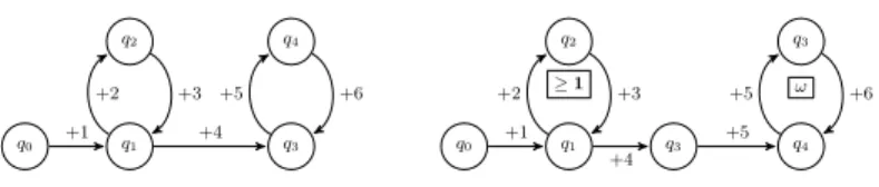
Lemma 4. Given a flat counter system S = hQ, Cn, ∆, li, the total number of minimal path schemas of S is finite and is smaller than card(∆)(2×card(∆)). This is a simple consequence of the fact that in a minimal path schema, each transition occurs at most twice. In Figure 1, we present a flat counter system S with a unique counter and one of its minimal path schemas. Each transition δi labelled by +i corresponds to a transition with the guard > and the update value +i. The minimal path schema shown in Figure 1 corresponds to the ω-regular expression δ1(δ2δ3)+δ4δ5(δ6δ5)ω. Note that in the representation of path schemas, a state may occur several times, as it is the case for q3 (this cannot occur in the representation of counter systems). Minimal path schemas play a crucial role in the sequel. Indeed, given a path schema P , there is a minimal path schema P0 such that every run respecting P respects P0 too. This can be easily
q0 q1 q2 q3 q4 q0 q1 q2 q3 q4 q3 ≥ 1 ω +1 +2 +3 +4 +5 +6 +1 +2 +3 +4 +5 +5 +6
Fig. 1. A flat counter system and one of its minimal path schemas
shown since whenever a maximal number of copies of a simple loop is identified as a factor of p1l1· · · pklk, this factor is replaced by the simple loop unless it is already present in the path schema.
Finally, the conditions imposed on the structure of path schemas implies the following corollary which states that the number of minimal path schemas for a given flat counter system is at most exponential in the size of the system (see similar statements in [20]).
Corollary 5. Given a flat counter system S and a configuration c0, there is a finite set of minimal path schemas X of cardinality at most card(∆)(2×card(∆)) such that lab(c0) = lab(SP ∈XP, c0).
4.2 Complexity Results
We write CPS [resp. KPS] to denote the class of path schemas from counter systems [resp. the class of path schemas from Kripke structures]. As a preliminary step, we consider the problem MC(PLTL[∅], KPS) that takes as inputs a path schema P in KPS, and φ ∈ PLTL[∅] and asks whether there is a run respecting P that satisfies φ. Let ρ and ρ0 be runs respecting P . For α ≥ 0, we write ρ ≡α ρ0
def
⇔ for every i ∈ [1, nbloops(P ) − 1], we have Min(iterP(ρ)[i], α) = Min(iterP(ρ0)[i], α). We state below a result concerning the runs of flat counter systems when respecting the same path schema.
Proposition 6. Let S be a flat counter system, P be a path schema, and φ ∈ PLTL[∅]. For all runs ρ and ρ0 respecting P such that ρ ≡
2td (φ)+5 ρ0, we have ρ, 0 |= φ iff ρ0, 0 |= φ.
This property can be proved by applying Theorem 3 repeatedly in order to get rid of the unwanted iterations of the loops. Our algorithm for MC(PLTL[∅], KPS) takes advantage of a result from [18] for model-checking ultimately periodic models with formulae from Past LTL. An ultimately periodic path is an infi-nite word in ∆ω of the form uvω were uv is a path segment and consequently first (v) = last (v). According to [18], given an ultimately periodic path w, and a formula φ ∈ PLTL[∅], the problem of checking whether there exists a run ρ such that lab(ρ) = w and ρ, 0 |= φ is in PTime (a tighter bound of NC can be obtained by combining results from [15] and Theorem 3).
The proof is a consequence of Proposition 6 and [18]. Indeed, given φ ∈ PLTL[∅] and P = p1l1+p2l2+. . . pklωk, first guess m ∈ [1, 2td (φ) + 5]
k−1 and check whether ρ, 0 |= φ where ρ is the obvious ultimately periodic word such that lab(ρ) = p1l
m[1] 1 p2l
m[2]
2 . . . pklkω. Since m is of polynomial size and ρ, 0 |= φ can be checked in polynomial time by [18], we get the NP upper bound.
From [16], we have the lower bound for MC(PLTL[∅], KPS).
Lemma 8. [16] MC(PLTL[∅], KPS) is NP-hard even if restricted to X and F. For a fixed n ∈ N, we write MC(PLTL[∅], KPS(n)) to denote the restriction of MC(PLTL[∅], KPS) to path schemas with at most n loops. When n is fixed, the number of ultimately periodic paths w in L(P ) such that each loop (except the last one) is visited is at most 2td (φ) + 5 times is bounded by (2td (φ) + 5)n, which is polynomial in the size of the input (because n is fixed).
Theorem 9. MC(PLTL[∅], KPS) is NP-complete. Given a fixed n ∈ N, MC(PLTL[∅], KPS(n)) is in PTime.
Note that it can be proved that MC(PLTL[∅], KPS(n)) is in NC, hence giving a tighter upper bound for the problem. This can be obtained by observing that we can run the NC algorithm for model checking PLTL[∅] over ultimately periodic paths parallelly on (2td (φ) + 5)n (polynomially many) different paths.
Now, we present how to solve MC(PLTL[∅], KF S) using Lemma 7. From Lemma 4, we know that the number of minimal path schemas in a flat Kripke structure S = hQ, ∆, li is finite and the length of a minimal path schema is at most 2 × card(∆). Hence, for solving the model-checking problem for a state q and a PLTL[∅] formula φ, a possible algorithm consists in choosing non-deterministically a minimal path schema P starting at q and then apply the algorithm used to establish Lemma 7. This new algorithm would be in NP. Fur-thermore, thanks to Corollary 5, we know that if there exists a run ρ of S such that ρ, 0 |= φ then there exists a minimal path schema P such that ρ respects P . Consequently there is an algorithm in NP to solve MC(PLTL[∅], KFS). Theorem 10. MC(PLTL[∅], KF S) is NP-complete.
NP-hardness can be established as a variant of the proof of Lemma 8.
Similarly, CPS(k) denotes the class of path schemas obtained from flat counter systems with number of loops bounded by k.
Lemma 11. For k ≥ 2, MC(PLTL[C], CPS(k)) is NP-hard.
The proof by reduction from SAT and it is less straightforward than the proof for Lemma 8 or the reduction presented in [16] when path schemas are involved. Indeed, we cannot encode the nondeterminism in the structure itself and the structure has only a constant number of loops. Actually, we cannot use a separate loop for each counter; the reduction is done by encoding the nondeterminism in the (possibly exponential) number of times a single loop is taken, and then using its binary encoding as an assignment for the propositional variables. Hence, the reduction uses in an essential way the counter values and the arithmetical constraints in the formula. By contrast, MC(PLTL[C], CPS(1)) can be shown in PTime.
5
Model-checking PLTL[C] over Flat Counter Systems
In this section, we provide a nondeterministic polynomial-time algorithm to solve MC(PLTL[C], CF S) (see Algorithm 1). To do so, we combine Theorem 3 with small solutions of constraint systems.
5.1 Characterizing Runs by System of Equations
In this section, we show how to build a system of equations from a path schema P and a configuration c0 such that the system of equations encodes the set of all runs respecting P from c0. This can be done for path schemas without disjunctions in guards that satisfy an additional validity property. A path schema P = p1l1+p2l2+. . . pklkω is valid whenever effect (lk)[i] ≥ 0 for every i ∈ [1, n] (see Section 4 for the definition of effect (lk)) and if all the guards in transitions in lk are conjunctions of atomic guards, then for each guard occurring in the loop lk of the form Piaixi ∼ b with ∼∈ {≤, <} [resp. with ∼∈ {=}, with ∼∈ {≥, >}] , we have P
iai× effect (lk)[i] ≤ 0 [resp.Piai× effect (lk)[i] = 0, P
iai× effect (lk)[i] ≥ 0]. It is easy to check that these conditions are necessary to visit the last loop lkinfinitely. More specifically, if a path schema is not valid, then no infinite run can respect it. Moreover, given a path schema, one can decide in polynomial time whether it is valid.
Now, let us consider a (not necessarily minimal) valid path schema P = p1l+1p2l+2 . . . pklωk (k ≥ 1) obtained from a flat counter system S such that all the guards on transitions are conjunctions of atomic guards of the formP
iaixi∼ b where ai∈ Z, b ∈ Z and ∼∈ {=, ≤, ≥, <, >}. Hence, disjunctions are disallowed in guards. The goal of this section (see Lemma 12 below) is to characterize the set iterP(c0) ⊆ Nk−1for some configuration c0as the set of solutions of a constraint system. For each loop li, we introduce a variable yi, whence the number of variables of the system/formula is precisely k − 1. A constraint system E over the set of variables {y1, . . . , yn} is a quantifier-free Presburger formula built over {y1, . . . , yn} as a conjunction of atomic constraints of the formPiaiyi∼ b where ai, b ∈ Z and ∼∈ {=, ≤, ≥, <, >}. Conjunctions of atomic counter constraints and constraint systems are essentially the same objects but the distinction allows to emphasize the different purposes: guard on counters in operational models and symbolic representation of sets of tuples.
Lemma 12. Let S = hQ, Cn, ∆, li be a flat counter system without disjunctions in guards, P be a valid path schema and c0 be a configuration. One can compute in polynomial time a constraint system E such that the set of solutions of E is equal to iterP(c0), E has nbloops(P ) − 1 variables, E has at most len(P ) × 2 × size(S)2 conjuncts and the greatest absolute value from constants in E is bounded by n × nbloops(P ) × K4× len(P )3where K is the greatest absolute value for constants occurring in S.
5.2 Elimination of Arithmetical Constraints and Disjunctions As stated in Lemma 12, the procedure for characterizing infinite runs in a counter system by a system of equations works only for a flat counter system with no
disjunction in guards (convexity of guards is essential). In this section, we show how to obtain such a system from a general flat counter system. Given a flat counter system S = hQ, Cn, ∆, li, a configuration c0 = hq0, v0i and a minimal path schema P starting from the configuration c0, we show that it is possible to build a finite set YP of path schemas such that (1) each path schema in YP has transitions without disjunctions in guards, (2) existence of a run ρ respecting P is equivalent to the existence of a path schema in YP having a run similar to ρ respecting it and (3) each path schema in YP is obtained from P by unfolding loops so that the terms in each loop satisfy the same atomic guards. Note that disjunctions could be easily eliminated at the cost of adding new transitions between states but this type of transformation may easily destroy flatness. Hence, the necessity to present a more sophisticated elimination procedure
We first introduce a few definitions. A (syntactic) resource R is a triple hX, T, Bi such that X is a finite set of propositional variables, T is a finite set of terms t appearing in some guards of the form t ∼ b (with b ∈ Z) and B is a finite set of integers. We say that a resource R = hX, T, Bi is coherent with a counter system S [resp. with a path schema P ] if B contains all the constants b occurring in guards of S [resp. of P ] of the form t ∼ b and T contains all the terms t occurring in guards of S [resp. of P ] of the form t ∼ b. The resource R is coherent with a formula φ ∈ PLTL[C], whenever the atomic formulae of φ are either of the form p ∈ X or t ∼ b with t ∈ T and b ∈ B. In the sequel, we assume that the considered resource is always coherent with S.
Assuming that B = {b1, . . . , bm} with b1 < · · · < bm, we write I to de-note the finite set of intervals I = {(−∞, b1− 1], [b1, b1], [b1+ 1, b2− 1], [b2, b2], · · · , [bm, bm], [bm+ 1, ∞)}. Note that I contains exactly 2m + 1 intervals. A term map m is a map m : T → I that abstracts term values. A footprint is an ab-straction of a model for PLTL[C] restricted to elements from the resource R: it is of the form ft : N → 2X× IT where I is the set of intervals built from B. The satisfaction relation |= involving models or runs can be adapted to footprints as follows (formulae and footprints are from the same resource):
– ft, i |=symbp def ⇔ p ∈ π1(ft(i)); ft, i |=symbt ≥ b def ⇔ π2(ft(i))(t) ⊆ [b, +∞), – ft, i |=symbt ≤ b def ⇔ π2(ft(i))(t) ⊆ (−∞, +b], – ft, i |=symbXφ def ⇔ ft, i + 1 |=symbφ, – ft, i |=symbφUψ def
⇔ ∃j ≥ i s.t. ft, j |=symbψ and ∀j0 ∈ [i, j − 1], ft, j0 |=symbφ. We omit the other obvious clauses. |=symb is the satisfaction relation for Past LTL when arithmetical constraints are understood as abstract propositions. Let R = hX, T, Bi be a resource and ρ = hq0, v0i, hq1, v1i · · · be an infinite run of S. The footprint of ρ with respect to R is the footprint ft(ρ) such that for i ≥ 0, we have ft(ρ)(i)def= hl(qi) ∩ X, mii where for every term t =Pjajxj∈ T , we have P
jajvi[j] ∈ mi(t). Note thatPjajvi[j] belongs to a unique element of I since I is a partition of Z. Hence, this definition makes sense. Lemma 13 below roughly states that satisfaction of a formula on a run can be checked symbolically from the footprint (this is useful for the correctness of forthcoming Algorithm 1).
Lemma 13. Let φ be in PLTL[C], R = hX, T, Bi be coherent with φ, ρ = hq0, v0i, hq1, v1i · · · be an infinite run and i ≥ 0. (I) Then ρ, i |= φ iff ft(ρ), i |=symb φ. (II) If ρ0 is an infinite run s.t. ft(ρ) = ft(ρ0), then ρ, i |= φ iff ρ0, i |= φ. In [6] we explain in details how to build a set YP of path schemas without disjunctions from a minimal path schema P , an initial configuration hq0, v0i and a resource R. The main idea of this construction consists in adding to the control states of path schemas some information on the intervals to which be-longs each term of T . In fact, in the transitions appearing in path schemas of YP the states belong to Q0 = Q × IT. Before stating the properties of YP, we introduce some notations. Given t = Pjajxj ∈ T , u ∈ Zn and a term map m, we write ψ(t, u, m(t)) to denote the formula below (b, b0 ∈ B): ψ(t, u, (−∞, b])def=P jaj(xj+u(j)) ≤ b; ψ(t, u, [b, +∞)) def =P jaj(xj+u(j)) ≥ b and ψ(t, u, [b, b0]) = ((P jaj(xj + u(j)) ≤ b0) ∧ ((Pjaj(xj+ u(j)) ≥ b). We write G?(T, B, U ) to denote the set of guards of the form ψ(t, u, m(t)) where t ∈ T , U is the finite set of updates from P and m : T → I. Each guard in G?(T, B, U ) is of linear size in the size of P . We denote ˜∆ the set of transitions Q0× G?(T, B, U ) × U × Q0. Note that the transitions in ˜∆ do not contain guards with disjunctions and ˜∆ is finite. We also define a function proj which associates to w ∈ ˜∆ω
the ω-sequence proj(w) : N → 2X × IT
such that for all i ∈ N, if w(i) = hhq, mi, g, u, hq0, m0ii and l(q) ∩ X = L then proj(w)(i)def
= hL, mi. We show that it is possible to build a finite set YP of path schemas over ˜∆ such that if P0 = p01(l01)+p0
2(l02)+. . . p0k0(l0k0)ω is a path schema in YP and ρ is a run hhq0, m0i, v0i −→ hhq1, m1i, v1i −→ hhq2, m2i, v2i · · · respecting P0 we have that proj(lab(ρ)) = ft(ρ). This point will be useful for Algorithm 1. The following theorem lists the main properties of the set YP.
Theorem 14. Given a flat counter system S, a minimal path schema P , a resource R = hX, T, Bi coherent with P and a configuration hq0, v0i, there is a finite set of path schemas YP over ˜∆ satisfying (1)–(6) below.
1. No path schema in YP contains guards with disjunctions in it. 2. There exists a polynomial q?(·) such that for every P0 ∈ Y
P, len(P0) ≤ q?(len(P ) + card(T ) + card(B)).
3. Checking whether a path schema P0 over ˜∆ belongs to YP can be done in polynomial time in size(P ) + card(T ) + card(B).
4. For every run ρ respecting P and starting at hq0, v0i, we can find a run ρ0 respecting some P0 ∈ YP such that ρ |= φ iff ρ0|= φ for every φ built over R. 5. For every run ρ0 respecting some P0 ∈ YP with initial values v0, we can find
a run ρ respecting P such that ρ |= φ iff ρ0|= φ for every φ built over R. 6. For every ultimately periodic word w · uω ∈ L(P0), for every φ built over R
checking whether proj(w · uω), 0 |=symb φ can be done in polynomial time in the size of w · u and in the size of φ.
5.3 Main Algorithm
In Algorithm 1 below, a polynomial p?(·) is used. We can define polynomial p?(·) using the small solutions for constraint systems [2], see details in [6]. Note that
y0 is a refinement of y (for all i, we have y0[i] ≈2td(φ)+5 y[i]) in which counter values are taken into account.
Algorithm 1 The main algorithm in NP with inputs S, c0= hq, v0i, φ
1: guess a minimal path schema P of S
2: build a resource R = hX, T, Bi coherent with P and φ 3: guess a valid schema P0 = p1l+1p2l
+ 2 . . . pkl
ω
k such that len(P 0
) ≤ q?(len(P ) + card(T ) + card(B))
4: guess y ∈ [1, 2td(φ) + 5]k−1; guess y0∈ [1, 2p?(size(S)+size(c0)+size(φ))]k−1
5: check that P0belongs to YP 6: check that proj(p1ly[1]1 p2l
y[2] 2 . . . l y[k−1] k−1 pkl ω k), 0 |=symbφ
7: build E over y1, . . . , yk−1 for P0 with initial values v0 (obtained from Lemma 12) 8: for i = 1 → k − 1 do
9: if y[i] = 2td(φ) + 5 then ψi← “yi≥ 2td(φ) + 5” else ψi← “yi= y[i]” 10: end for
11: check that y0|= E ∧ ψ1∧ · · · ∧ ψk−1
Algorithm 1 starts by guessing a path schema P (line 1) and an unfolded path schema P0 = p1l+1p2l+2 . . . pklωk (line 3) and check whether P
0 belongs to YP (line 5). It remains to check whether there is a run ρ respecting P0 such that ρ |= φ. Suppose there is such a run ρ; let y be the unique tuple in [1, 2td(φ) + 5]k−1 such that y ≈
2td(φ)+5 iterP0(ρ). By Proposition 6, we have
proj(p1l y[1] 1 p2l y[2] 2 . . . l y[k−1]
k−1 pklωk), 0 |=symb φ. Since the set of tuples of the form iterP0(ρ) is characterized by a system of equations, by the existence of small
so-lutions from [2], we can assume that iterP0(ρ) contains only small values. Hence
line 4 guesses y and y0(corresponding to iterP0(ρ) with small values). Line 6
pre-cisely checks proj(p1l y[1] 1 p2l y[2] 2 . . . l y[k−1] k−1 pkl ω
k), 0 |=symbφ whereas line 11 checks whether y0 encodes a run respecting P0 with y0≈2td(φ)+5y.
Lemma 15. Algorithm 1 runs in nondeterministic polynomial time. It remains to check that Algorithm 1 is correct.
Lemma 16. S, c0|= φ iff Algorithm 1 on inputs S, c0, φ has an accepting run. In the proof of Lemma 16, we take advantage of all our preliminary results. Proof. By way of example, we show that if Algorithm 1 on inputs S, c0= hq0, v0i, φ has an accepting computation, then S, c0|= φ. This means that there are P , P0, y, y0that satisfy all the checks. Let w = p1l
y0[1]
1 · · · pk−1l y0[k−1]
k−1 pklωk and ρ = hhq0, m0i, v0ihhq1, m1i, x1ihhq2, m2i, x2i · · · ∈ (Q0× Zn)ωbe defined as follows: for every i ≥ 0, qi
def
= π1(source(w(i))), and for every i ≥ 1, we have xi
def
= xi−1+ update(w(i)). By Lemma 12, since y0|= E ∧ ψ1∧ · · · ∧ ψk−1, ρ is a run respecting P0starting at the configuration hhq0, m0i, v0i. Since y0|= ψ1∧· · ·∧ψk−1and y |= ψ1∧· · ·∧ψk−1, by Proposition 6, (z) proj(p1l y[1] 1 p2l y[2] 2 . . . l y[k−1] k−1 pklωk), 0 |=symbφ, iff (zz) proj(p1l y0[1] 1 p2l y0[2] 2 . . . l y0[k−1]
k−1 pklωk), 0 |=symb φ. Algorithm 1 guarantees that proj(p1l y[1] 1 p2l y[2] 2 . . . l y[k−1]
k−1 pklωk), 0 |=symb φ, whence we have (zz). Since proj(p1l y0[1] 1 p2l y0[2] 2 . . . l y0[k−1] k−1 pkl ω
φ. By Theorem 14(5), there is an infinite run ρ0, starting at the configuration hq0, v0i and respecting P , such that ρ0, 0 |= φ.
For the other direction, see [6]. ut
As a corollary, we can state the main result of the paper. Theorem 17. MC(PLTL[C], CF S) is NP-complete.
6
Conclusion
Classes of Systems PLTL[∅] PLTL[C] Reachability
KPS NP-complete —– PTime
See [16] for X and U
CPS NP-complete NP-complete (Theo. 17) NP-complete KPS(n) PTime (Theo. 9) —– PTime CPS(n), n > 1 ?? NP-complete (Lem. 11) ??
CPS(1) PTime PTime PTime
KF S NP-complete —– PTime
See [16] for X and U
CF S NP-complete NP-complete (Theo. 17) NP-complete
We have investigated the computational complexity of the model-checking problem for flat counter systems with formulae from an enriched version of LTL. Our main result is the NP-completeness of MC(PLTL[C], CFS), significantly improving the complexity upper bound from [7]. This also improves the results about the effective semilinearity of the reachability relations for such flat counter systems from [5,11] and it extends the recent result on the NP-completeness of model-checking flat Kripke structures with LTL from [16] by adding counters and past-time operators. Our main results are presented above and compared to the reachability problem.
As far as the proof technique is concerned, the NP upper bound is obtained as a combination of a general stuttering property for LTL with past-time operators (a result extending what is done in [17] with past-time operators) and the use of small integer solutions for quantifier-free Presburger formulae [2]. There are several related problems which are not addressed in the paper. For instance, the extension of the model-checking problem to full CTL? is known to be decid-able [7] but the characterization of its exact complexity is open.
References
1. B. Boigelot. Symbolic methods for exploring infinite state spaces. PhD thesis, Université de Liège, 1998.
2. I. Borosh and L. Treybig. Bounds on positive integral solutions of linear Diophan-tine equations. American Mathematical Society, 55:299–304, 1976.
3. M. Bozga, R. Iosif, and F. Konecný. Fast acceleration of ultimately periodic rela-tions. In CAV’10, volume 6174 of LNCS, pages 227–242. Springer, 2009.
4. H. Comon and V. Cortier. Flatness is not a weakness. In CSL’00, volume 1862 of LNCS, pages 262–276. Springer, 2000.
5. H. Comon and Y. Jurski. Multiple counter automata, safety analysis and PA. In CAV’98, volume 1427 of LNCS, pages 268–279. Springer, 1998.
6. S. Demri, A. Dhar, and A. Sangnier. Taming past LTL and flat counter systems. Technical report, 2012. ArXiv.
7. S. Demri, A. Finkel, V. Goranko, and G. van Drimmelen. Model-checking CTL∗ over flat Presburger counter systems. JANCL, 20(4):313–344, 2010.
8. C. Dixon, M. Fisher, and B. Konev. Temporal logic with capacity constraints. In FROCOS’07, volume 4720 of LNCS, pages 163–177. Springer, 2007.
9. J. Esparza, A. Finkel, and R. Mayr. On the verification of broadcast protocols. In LICS’99, pages 352–359, 1999.
10. K. Etessami and T. Wilke. An until hierarchy and other applications of an Ehrenfeucht-Fraïssé game for temporal logic. I&C, 160(1–2):88–108, 2000. 11. A. Finkel and J. Leroux. How to compose Presburger accelerations: Applications
to broadcast protocols. In FST&TCS’02, volume 2256 of LNCS, pages 145–156. Springer, 2002.
12. A. Finkel, E. Lozes, and A. Sangnier. Towards model-checking programs with lists. In Infinity in Logic & Computation, volume 5489 of LNAI, pages 56–82. Springer, 2009.
13. D. Gabbay. The declarative past and imperative future. In Temporal Logic in Specification, Altrincham, UK, volume 398 of LNCS, pages 409–448. Springer, 1987. 14. C. Haase, S. Kreutzer, J. Ouaknine, and J. Worrell. Reachability in succinct and parametric one-counter automata. In CONCUR’09, volume 5710 of LNCS, pages 369–383. Springer, 2009.
15. L. Kuhtz. Model Checking Finite Paths and Trees. PhD thesis, Universität des Saarlandes, 2010.
16. L. Kuhtz and B. Finkbeiner. Weak Kripke structures and LTL. In CONCUR’11, volume 6901 of LNCS, pages 419–433. Springer, 2011.
17. A. Kučera and J. Strejček. The stuttering principle revisited. Acta Informatica, 41(7–8):415–434, 2005.
18. F. Laroussinie, N. Markey, and P. Schnoebelen. Temporal logic with forgettable past. In LICS’02, pages 383–392. IEEE, 2002.
19. F. Laroussinie and P. Schnoebelen. Specification in CTL + past for verification in CTL. I&C, 156:236–263, 2000.
20. J. Leroux and G. Sutre. Flat counter systems are everywhere! In ATVA’05, volume 3707 of LNCS, pages 489–503. Springer, 2005.
21. C. Lutz. NEXPTIME-complete description logics with concrete domains. In IJ-CAR’01, volume 2083 of LNCS, pages 46–60. Springer, 2001.
22. M. Minsky. Computation, Finite and Infinite Machines. Prentice Hall, 1967. 23. D. Peled and T. Wilke. Stutter-invariant temporal properties are expressible
with-out the next-time operator. IPL, 63:243–246, 1997.
24. C. Rackoff. The covering and boundedness problems for vector addition systems. TCS, 6(2):223–231, 1978.