Robust nonparametric estimation of the conditional tail dependence coefficient

HAL Id: hal-02269476

https://hal.archives-ouvertes.fr/hal-02269476

Preprint submitted on 22 Aug 2019

HAL is a multi-disciplinary open access

archive for the deposit and dissemination of sci-entific research documents, whether they are pub-lished or not. The documents may come from teaching and research institutions in France or

L’archive ouverte pluridisciplinaire HAL, est destinée au dépôt et à la diffusion de documents scientifiques de niveau recherche, publiés ou non, émanant des établissements d’enseignement et de recherche français ou étrangers, des laboratoires

Robust nonparametric estimation of the conditional tail

dependence coefficient

Yuri Goegebeur, Armelle Guillou, Nguyen Khanh Le Ho, Jing Qin

To cite this version:

Yuri Goegebeur, Armelle Guillou, Nguyen Khanh Le Ho, Jing Qin. Robust nonparametric estimation of the conditional tail dependence coefficient. 2019. �hal-02269476�

Robust nonparametric estimation of the conditional tail

dependence coefficient

Yuri Goegebeurp1q_{, Armelle Guillou}p2q_{, Nguyen Khanh Le Ho}p1q_{, Jing Qin}p1q

p1q _{Department of Mathematics and Computer Science, University of Southern Denmark, Campusvej}

55, 5230 Odense M, Denmark

p2q _{Institut Recherche Math´ematique Avanc´ee, UMR 7501, Universit´e de Strasbourg et CNRS, 7 rue}

Ren´e Descartes, 67084 Strasbourg cedex, France

Abstract

We consider robust and nonparametric estimation of the coefficient of tail dependence in presence of random covariates. The estimator is obtained by fitting the extended Pareto distribution locally to properly transformed bivariate observations using the minimum den-sity power divergence criterion. We establish convergence in probability and asymptotic normality of the proposed estimator under some regularity conditions. The finite sample performance is evaluated with a small simulation experiment, and the practical applicability of the method is illustrated on a real dataset of air pollution measurements.

Keywords: Coefficient of tail dependence, robustness, local estimation, empirical process.

1

Introduction

Many problems involving extreme events are inherently multivariate, and hence they should be handled with appropriate multivariate extreme value methods. Of particular interest is the estimation of the extremal dependence between two or more variables. A full characterization of the extremal dependence between variables can be obtained from functions like the spectral dis-tribution function or the Pickands dependence function. We refer to Beirlant et al. (2004), and de Haan and Ferreira (2006), and the references therein, for more details about this approach. Alternatively, similar to classical statistics one can try and summarize the extremal dependency in a number of well-chosen coefficients that give a representative picture of the full dependency structure, like, e.g., the coefficient of tail dependence (Ledford and Tawn, 1997). Modelling tail dependence is a critical issue in many scientific disciplines. For instance, in finance and actuarial science an important problem is to estimate very large quantiles of the distribution of the sums of possibly dependent risks (Barbe et al., 2006). In environmental science, study-ing dependence in extreme levels of pollutants like ozone, particulate matter, carbon monoxide and temperature is important as combined high levels of these variables may pose a major threat to human health (Escobar-Bach et al., 2018). In this paper, we will consider robust and nonparametric estimation of the coefficient of tail dependence when there are random covariates.

Let pYp1q_{, Y}p2q_{q be a bivariate random vector recorded along with a random covariate X P R}p_.

The covariate X has density function fX with support SX Ă Rp, having non-empty interior.

The continuous conditional marginal distribution functions of Ypjq_{given X “ x are denoted by}

Fjp¨|xq, j “ 1, 2, and the joint conditional distribution function of the pair satisfies that for all

x P SX and y P r0, 1s P ´ 1 ´ F1pYp1q|xq ă y, 1 ´ F2pYp2q|xq ă y ˇ ˇ ˇX “ x ¯ “ Cpxq y 1 ηpxq ˆ 1 ` 1 ηpxqδpy|xq ˙ ,

where ηpxq P p0, 1s is the conditional tail dependence coefficient, and |δp¨|xq| is a regularly vary-ing function in the neighborhood of zero with index τ pxq ą 0. In this paper we focus on the estimation of ηpxq, and introduce a nonparametric estimator, which is obtained from local fits of the above model in a neigborhood of x, a point of interest in the covariate space. In absence of covariates, several estimators for η have been introduced in the extreme value literature. We refer to Ledford and Tawn (1997), Peng (1999), Draisma et al. (2004), Beirlant et al. (2011), and Goegebeur and Guillou (2013), to name but a few.

Our aim in this paper is to estimate the conditional tail dependence coefficient in a robust way, in order to ensure that our estimation procedure works in the presence of possible outliers. To achieve this, we will use the idea of the density power divergence introduced by Basu et al. (1998). In particular, the density power divergence between density functions h and g is given by

∆αph, gq :“

# ş

R“g 1`α

pyq ´`1 `_α1˘ gαpyqhpyq ` 1<sub>α</sub>h1`αpyq‰ dy, α ą 0, ş

Rlog hpyq

gpyqhpyqdy, α “ 0.

(1)

Here h is assumed to be the true (typically unknown) density of the data, whereas g is a paramet-ric model, depending on a parameter vector θ which is determined by minimizing the empiparamet-rical version of (1). The resulting estimator will be called, in the sequel, minimum density power divergence (MDPD) estimator. In the present paper we will adjust this criterion to the local estimation context with focus on estimating conditional extreme dependence. Dutang et al. (2014) used this criterion to obtain a robust estimator for η, but in a context without covariates. To the best of our knowledge, robust nonparametric estimation of the conditional coefficient of tail dependence has not been considered so far in the extreme value literature.

The remainder of the paper is organized as follows. In Section 2, we simplify the problem to the case where the conditional marginal distributions are known and we prove the existence, convergence in probability and asymptotic normality of the MDPD estimator of the conditional tail dependence coefficient. Then in Section 3, the realistic situation where the margins are unknown is considered and similar results are established. The efficiency and robustness of our MDPD estimator are illustrated in a small simulation study in Section 4 and on a real dataset on air pollution in Section 5. Finally, all the proofs are postponed to the appendix.

2

Case of known margins

In this section, we assume that the conditional marginal distribution functions F1p¨|xq and

F2p¨|xq are known. Define Z :“ min ´ 1 1´F1pYp1q|Xq, 1 1´F2pYp2q|Xq ¯

. Direct computations yield for all x P SX

FZpz|xq :“ PpZ ą z|X “ xq “ Cpxqz´ 1 ηpxq ˆ 1 ` 1 ηpxqδZpz|xq ˙ , (2) where δZpz|xq :“ δ ˆ 1 z ˇ ˇ ˇx ˙ .

Here |δZp¨|xq| is a regularly varying function at infinity with index ´τ pxq, which is additionally

assumed to be normalized, i.e., such that δZpz|xq “ Apxq exp ˆżz 1 εpu|xq u du ˙ , (3)

with Apxq P R and εpz|xq Ñ ´τ pxq as z Ñ 8.

Note that the conditional distribution of Z, given X “ x, satisfies Condition pRq in Dierckx et al. (2014) with second order parameter ρpxq :“ ´τ pxqηpxq. Thus, one can approximate the conditional distribution of Z{u, given Z ą u, where u denotes a high threshold value, by the extended Pareto distribution given by

Gpz; η, δ, ρq “ $ & % 1 ´ ” z ´ 1 ` δ ´ δzρη ¯ı´1_η , z ą 1, 0, z ď 1,

and density function

gpz; η, δ, ρq “ $ & % z´ 1η ´1 η ” 1 ` δ ´ 1 ´ zρη ¯ı´1<sub>η</sub>´1” 1 ` δ ´ 1 ´ ´ 1 `ρ_η ¯ zρη ¯ı , z ą 1, 0, z ď 1,

where η ą 0, ρ ă 0, and δ ą maxt´1, η{ρu.

Indeed, as shown in Beirlant et al. (2009), we have sup zě1 ˇ ˇ ˇ ˇ FZpuz|xq FZpu|xq ´ Gpz; ηpxq, δZpu|xq, ρpxqq ˇ ˇ ˇ ˇ“ opδZpu|xqq if u Ñ 8.

Clearly, based on this result, one can obtain an estimator for ηpxq by fitting the extended Pareto distribution to the relative excesses over a high threshold.

Let pX1, Z1q, . . . , pXn, Znq be independent copies of the random vector pX, Zq. We develop a

nonparametric, robust and asymptotically unbiased estimator for ηpxq by fitting g locally to the relative excesses Zi{un, i “ 1, . . . , n, by means of the MDPD criterion, adjusted to locally

weighted estimation, i.e., we minimize p ∆αpη, δZ; ρq :“ 1 n n ÿ i“1 Khnpx ´ Xiq "ż8 1 g1`αpz; η, δZ, ρqdz ´ ˆ 1 ` 1 α ˙ gαˆ Zi un ; η, δZ, ρ ˙* 1l_tZiąunu, in case α ą 0 and p ∆0pη, δZ; ρq :“ ´ 1 n n ÿ i“1 Khnpx ´ Xiq ln g ˆ Zi un ; η, δZ, ρ ˙ 1ltZiąunu, in case α “ 0, where Khnpxq :“ Kpx{hnq{h p

n, K is a joint density function on Rp, hn is a

non-random sequence of bandwidths with hn Ñ 0 if n Ñ 8, 1ltAu is the indicator function on the

event A and unis a local non-random threshold sequence satisfying unÑ 8 if n Ñ 8. Note that

in case α “ 0, the local empirical density power divergence criterion corresponds with a locally weighted log-likelihood function. The parameter α controls the trade-off between efficiency and robustness of the MDPD criterion: the estimator becomes more efficient but less robust as α gets closer to zero, whereas for increasing α the robustness increases and the efficiency decreases. Note that we only estimate ηpxq and δZpun|xq with the MDPD criterion, while the second order

parameter ρpxq will be fixed at some value. Fixing second order parameters like ρpxq here at some value is a common practice in extreme value statistics, and was also proposed in Beirlant et al. (1999), Feuerverger and Hall (1999), and Gomes and Martins (2004). Alternatively, one can replace ρpxq by an external consistent estimator. However, the estimation of ρpxq in a robust way is still an open problem, and moreover, using an external consistent estimator rather than a canonical value, does not, in general, improve the performance of the final MDPD estimator in practice. For all these reasons, we only use a canonical value for the parameter ρpxq in the sequel. The MDPD estimators of pηpxq, δZpun|xqq satisfy the estimating equations

0 “ 1 n n ÿ i“1 Khnpx ´ Xiq1ltZiąunu ż8 1 gαpz; η, δZ, ρq Bgpz; η, δZ, ρq Bη dz ´1 n n ÿ i“1 Khnpx ´ Xiqg α´1ˆ Zi un ; η, δZ, ρ ˙_Bg ´ Zi un; η, δZ, ρ ¯ Bη 1ltZiąunu, (4) 0 “ 1 n n ÿ i“1 Khnpx ´ Xiq1ltZiąunu ż8 1 gαpz; η, δZ, ρqBgpz; η, δZ , ρq BδZ dz ´1 n n ÿ i“1 Khnpx ´ Xiqg α´1ˆ Zi un ; η, δZ, ρ ˙_Bg ´ Zi un; η, δZ, ρ ¯ BδZ 1l_tZiąunu. (5)

The following statistic is crucial for studying the asymptotic behavior of the estimators. Set ln`x :“ ln maxtx, 1u, x ą 0, and

TnpK, s, t|xq :“ 1 n n ÿ i“1 Khnpx ´ Xiq ˆ Zi un ˙sˆ ln` Zi un ˙t 1ltZiąunu,

where s ď 0 and t ě 0. The motivation for considering this type of statistic is that the estimat-ing equations (4) and (5) only depend on statistics of this form. Note that ln`x is introduced

to ensure that pln`Zi{unqt is always well defined (t is nonnegative, not necessary integer).

Due to the regression context, we need the following classical H¨older-type conditions. Here } ¨ } denotes some norm on Rp.

Assumption pHq There exist positive constants MfX, MC, MA, Mη, Mε, δfX, δC, δA, δη, and

δε, such that for all px, zq P SX ˆ SX:

|fXpxq ´ fXpzq| ď MfX}x ´ z} δ_fX, |Cpxq ´ Cpzq| ď MC}x ´ z}δC, |Apxq ´ Apzq| ď MA}x ´ z}δA, |ηpxq ´ ηpzq| ď Mη}x ´ z}δη, sup yě1 |εpy|xq ´ εpy|zq| ď Mε}x ´ z}δε.

Also, the following assumption, standard in the context of local estimation, is required on the kernel function.

Assumption pK1q K is a bounded density function on Rp, with support SK included in the unit

ball of Rp_.

In order to establish the asymptotic normality of the consistent sequence of solutions pηpnpxq, pδZ,npxqq of the estimating equations (4) and (5), we introduce

Spjqn psq :“ b nhpnFZpun|xqfXpxq « TnpK, s, j|xq FZpun|xqfXpxq ´ j!η j 0pxq r1 ´ sη0pxqsj`1 ff , j P t0, 1, 2, 3u,

where we denote by η0pxq, resp. ρ0pxq, the true conditional tail dependence coefficient, resp.

second order parameter.

Theorem 2.1 Let pX1, Z1q, . . . , pXn, Znq be a sample of independent copies of the random

vec-tor pX, Zq where the distribution of Z, given X “ x, satisfies (2) and (3), X follows a distribu-tion with density funcdistribu-tion fX, and assume pHq and pK1q hold. For all x P IntpSXq with fXpxq ą

0, we assume that un Ñ 8 and hn Ñ 0 in such a way that hδnεln unÑ 0, nhpnFZpun|xq Ñ 8,

b nhpnFZpun|xqδZpun|xq Ñ λ P R, b nhpnFZpun|xqh δ_fX^δC n Ñ 0, b nhpnFZpun|xqh δη n ln un Ñ 0. Then in C4prS, 0sq, S ă 0, pSp0qn , Sp1qn , Sp2qn , Snp3qq pSp0q, Sp1q, Sp2q, Sp3qq, for n Ñ 8,

a Gaussian process, with, for s P rS, 0s, mean functions ErSpjqpsqs “ ´λafXpxqj!η0j´1pxq „ 1 r1 ´ sη0pxqsj`1 ´ 1 ´ ρ0pxq r1 ´ ρ0pxq ´ sη0pxqsj`1  , j P t0, 1, 2, 3u,

and covariance functions given by CovpSpjqps1q, Spkqps2qq “ pj ` kq!η j`k 0 pxq}K}22 r1 ´ ps1` s2qη0pxqs1`j`k , pj, kq P t0, 1, 2, 3u2.

Note that Dierckx et al. (2014) obtained a similar result, though under their high level assump-tion called pMq, which is avoided in the present paper.

Based on this theorem, one can now establish the existence, convergence in probability and asymptotic normality of the MDPD estimators of pη0pxq, δZpun|xqq, when suitably normalized.

This theorem is similar to Theorems 2 and 3 in Dierckx et al. (2014) with our new conditions given in our Theorem 2.1, and thus the proof is omitted.

Theorem 2.2 Let pX1, Z1q, . . . , pXn, Znq be a sample of independent copies of the random

vec-tor pX, Zq where the distribution of Z, given X “ x, satisfies (2) and (3), X follows a distribu-tion with density funcdistribu-tion fX, and assume pHq and pK1q hold.

For all x P IntpSXq with fXpxq ą 0, let unÑ 8 and hnÑ 0 in such a way that nhpnFZpun|xq Ñ

8 and hδnη^δεln un Ñ 0. Then with probability tending to 1, there exists sequences of

solu-tions pηpnpxq, pδZ,npxqq of the estimating equations (4) and (5), with ρ fixed at ρ0pxq such that ppηnpxq, pδZ,npxqqÝÑ pηP 0pxq, 0q. If additionally, b nhpnFZpun|xq δZpun|xq ÝÑ λ P R, (6) b nhpnFZpun|xq h δ_fX^δC n ÝÑ 0, (7) b nhpnFZpun|xq hδnη ln un ÝÑ 0, (8) then b nhpnFZpun|xqfXpxq „ p ηnpxq ´ η0pxq p δZ,npxq ´ δZpun|xq  N2`0, C´1pρ0pxqqBpρ0pxqqΣpρ0pxqqB1pρ0pxqqC´1pρ0pxqq˘ ,

for n Ñ 8, where the matrix Bpρ0pxqq is defined by

Bpρ0pxqq :“ η´α´20 pxq » — – ´αη_r1`αp1`η0pxqp1`η0pxqq 0pxqqs2 η0pxq 0 ´1 ´<sub>r1`αp1`η</sub>αη0pxqρ0pxqp1`η0pxqq 0pxqqsr1´ρ0pxq`αp1`η0pxqqs η0pxq ´η0pxqp1 ´ ρ0pxqq 0 fi ffi fl,

the elements of the symmetric p4 ˆ 4q matrix Σpρ0pxqq are given by σ11pρ0pxqq :“ }K}22 σ21pρ0pxqq :“ }K} 2 2 1 ` αp1 ` η0pxqq σ22pρ0pxqq :“ }K} 2 2 1 ` 2αp1 ` η0pxqq σ31pρ0pxqq :“ }K} 2 2 1 ´ ρ0pxq ` αp1 ` η0pxqq σ32pρ0pxqq :“ }K} 2 2 1 ´ ρ0pxq ` 2αp1 ` η0pxqq σ33pρ0pxqq :“ }K} 2 2 1 ´ 2ρ0pxq ` 2αp1 ` η0pxqq σ41pρ0pxqq :“ η0pxq}K}22 r1 ` αp1 ` η0pxqqs2 σ42pρ0pxqq :“ η0pxq}K}22 r1 ` 2αp1 ` η0pxqqs2 σ43pρ0pxqq :“ η0pxq}K}22 r1 ´ ρ0pxq ` 2αp1 ` η0pxqqs2 σ44pρ0pxqq :“ 2η2₀pxq}K}22 r1 ` 2αp1 ` η0pxqqs3

and those of the symmetric p2 ˆ 2q matrix Cpρ0pxqq by

C11pρ0pxqq :“ η´α´20 pxq 1 ` α2p1 ` η0pxqq2 r1 ` αp1 ` η0pxqqs3 C21pρ0pxqq :“ η´α´20 pxq ρ0pxqp1 ´ ρ0pxqqr1 ` αp1 ` η0pxqq ` α2p1 ` η0pxqq2s ` α3ρ0pxqp1 ` η0pxqq3 r1 ` αp1 ` η0pxqqs2r1 ´ ρ0pxq ` αp1 ` η0pxqqs2 C22pρ0pxqq :“ η´α´20 pxq p1 ´ ρ0pxqqρ20pxq ` αρ20pxqp1 ` η0pxqqrαp1 ` η0pxqq ´ ρ0pxqs r1 ` αp1 ` η0pxqqsr1 ´ ρ0pxq ` αp1 ` η0pxqqsr1 ´ 2ρ0pxq ` αp1 ` η0pxqqs . Note that the expected value of the limiting random vector in Theorem 2.2 is zero, whatever the value of λ. The estimator is therefore said to be asymptotically unbiased.

The following proposition deals with the behavior of the MDPD estimators ppηnpxq, pδZ,npxqq when the parameter ρpxq is fixed at some value ρ ă 0, possibly mis-specified.r

Proposition 2.1 Under the assumptions of Theorem 2.2, but now with ρ fixed at ρ in the es-r timating equation (4) and (5), with probability tending to 1, there exists sequences of solutions pηpnpxq, pδZ,npxqq of the estimating equations such that pηpnpxq, pδZ,npxqq

P

If additionally (6), (7) and (8) hold, then b nhpnFZpun|xqfXpxq „ p ηnpxq ´ η0pxq p δZ,npxq  N2 ´ ´λafXpxqC´1prρqBprρqD, C´1prρqBprρqΣpρqBr 1 prρqC´1prρq ¯ , for n Ñ 8, where the elements of the vector D are the following

D1 :“ 0 D2 :“ ´ αρ0pxqp1 ` η0pxqq η0pxqr1 ` αp1 ` η0pxqqsr1 ´ ρ0pxq ` αp1 ` η0pxqqs D3 :“ ´ rαp1 ` η0pxqq ´ρsρr 0pxq η0pxqr1 ´ρ ` αp1 ` ηr 0pxqqsr1 ´ ρ0pxq ´ρ ` αp1 ` ηr 0pxqqs D4 :“ ρ0pxqp1 ´ ρ0pxqq ´ α2ρ0pxqp1 ` η0pxqq2 r1 ` αp1 ` η0pxqqs2r1 ´ ρ0pxq ` αp1 ` η0pxqqs2 .

Again the proof of Proposition 2.1 is similar to the one of Proposition 1 in Dierckx et al. (2014) and thus is omitted. Note that in caseρ is mis-specified, then the mean of the limiting normalr distribution is not necessarily zero, and hence one possible loses the asymptotic unbiasedness. However, as will be clear from the simulations, even though ρ is mis-specified, the proposedr MDPD estimator performs well with respect to bias. Also note that the asymptotic variance expression in Proposition 2.1 is the same as that in Theorem 2.2, though with ρ0pxq replaced byρ.r

3

Case of unknown margins

In this section, we consider the general framework where both F1p¨|xq and F2p¨|xq are unknown

conditional distribution functions. We want to mimic what has been done in the previous section. To this aim, we define

q Z :“ min ˆ 1 1 ´ Fn,1pYp1q|Xq , 1 1 ´ Fn,2pYp2q|Xq ˙ ,

for suitable estimators Fn,j of Fj, j “ 1, 2. Then similarly as in the previous section, the statistic

q TnpK, s, t|xq :“ 1 n n ÿ i“1 Khnpx ´ Xiq ˜ q Zi un ¸s˜ ln` q Zi un ¸t 1l_{t qZ} iąunu,

is the cornerstone for the MDPD estimator, denotedηqnpxq. In particular, the main result relies essentially on the asymptotic properties of this statistic, and so the idea will be to decompose

b nhpnFZpun|xqfXpxq « q TnpK, s, j|xq FZpun|xqfXpxq ´ j!η j 0pxq r1 ´ sη0pxqsj`1 ff

into the two terms b nhpnFZpun|xqfXpxq « TnpK, s, j|xq FZpun|xqfXpxq ´ j!η j 0pxq r1 ´ sη0pxqsj`1 ff ` b nhpnFZpun|xqfXpxq « q TnpK, s, j|xq FZpun|xqfXpxq ´ TnpK, s, j|xq FZpun|xqfXpxq ff . (9)

The first term can be dealt with using the results from the previous section, whereas we have to show that the second term is negligible for all s ă 0 with j P t0, 1, 2, 3u or ps, jq “ p0, 0q. In the sequel, we will use the empirical kernel estimator of the unknown distribution functions

Fn,jpy|xq :“ řn i“1Kcpx ´ Xiq1ltY_ipjqďyu řn i“1Kcpx ´ Xiq , j “ 1, 2,

where the bandwidth c :“ cn is a positive non-random sequence satisfying cn Ñ 0 as n Ñ 8.

Here we kept the same kernel K as in the divergence objective function, but of course any other kernel function can be used.

Before stating our main results, we need to impose again some assumptions, in particular a H¨older-type condition on each conditional marginal distribution function Fj similar to those

imposed in Section 2.

Assumption pF q. There exist MFj ą 0 and δFj ą 0 such that |Fjpy|xq ´ Fjpy|zq| ď MFj}x ´

z}δFj_{, for all y P R and all px, zq P S}

Xˆ SX, and j “ 1, 2.

Concerning the kernel K a stronger assumption than pK1q is needed. Denote by Bzprq the closed

ball with center z and radius r with respect to }.}.

Assumption pK2q. K satisfies Assumption pK1q, there exists δ, m ą 0 such that B0pδq Ă SK

and Kpuq ě m for all u P B0pδq, and K belongs to the linear span (the set of finite

lin-ear combinations) of functions k ě 0 satisfying the following property: the subgraph of k, tps, uq : kpsq ě uu, can be represented as a finite number of Boolean operations among sets of the form tps, uq : qps, uq ě ϕpuqu, where q is a polynomial on Rpˆ R and ϕ is an arbitrary real function.

The latter assumption has already been used in Gin´e and Guillou (2002) or Gin´e et al. (2004). In particular, it allows us to measure the discrepancy between the conditional distribution function Fjand its empirical kernel version Fn,j, as stated in the following lemma established by

Escobar-Bach et al. (2018).

Lemma 3.1 Assume that there exists b ą 0 such that f pxq ě b, @x P SX Ă Rp, f is bounded,

and pK2q and pF q hold. Consider a sequence c tending to 0 as n Ñ 8 such that for some q ą 1

| log c|q

Also assume that there exists an ε ą 0 such that for n sufficiently large inf

xPSX

λ ptu P B0p1q : x ´ cu P SXuq ą ε,

where λ denotes the Lebesgue measure. Then, for any 0 ă δ ă minpδF1, δF2q, we have

sup py,xqPRˆSX |Fn,jpy|xq ´ Fjpy|xq| “ oP ˜ max ˜c | log c|q ncp , c δ ¸¸ , for j “ 1, 2. We are now able to study the second term in (9).

Theorem 3.1 Let pX1, Z1q, . . . , pXn, Znq be a sample of independent copies of the random

vector pX, Zq where the distribution of Z, given X “ x, satisfies (2) and (3), X follows a distribution with a bounded density function fX, and such that there exists b ą 0 satisfying

f pxq ě b, @x P SX Ă Rp. Assume also Assumptions pHq, pK2q and pF q.

Consider now a sequence c tending to 0 as n Ñ 8 such that for some q ą 1 | log c|q

ncp ÝÑ 0.

Also assume that there exists an ε ą 0 such that for n sufficiently large inf

xPSX

λ ptu P B0p1q : x ´ cu P SXuq ą ε,

where λ denotes the Lebesgue measure. Let un Ñ 8 and hn Ñ 0 in such a way that for any

δ P p0, minpδF1, δF2qq nhp_nrn:“ nhpnmax ˜c | log c|q ncp , c δ ¸ ÝÑ 0 (10) nhp_nFZpun|xq ÝÑ 8, (11)

then for any s ă 0 with j P t0, 1, 2, 3u or ps, jq “ p0, 0q, we have d nhpn FZpun|xqfXpxq ” q TnpK, s, j|xq ´ TnpK, s, j|xq ı “ oPp1q.

Using Theorem 3.1 we can now establish the main theorem of this paper, stating consistency and asymptotic normality of the conditional η estimator, in case of general conditional marginal distribution functions, which are estimated with kernel estimators.

Theorem 3.2 Under the same assumptions as in Theorem 3.1, let x P IntpSXq and suppose

that hδnη^δεln un Ñ 0. Then with probability tending to 1, there exists sequences of solutions

pqηnpxq, qδZ,npxqq of the estimating equations (4) and (5) such that pqηnpxq, qδZ,npxqqÝÑ pηP 0pxq, 0q.

If additionally (6), (7) and (8) hold, then b nhpnFZpun|xqfXpxq „ q ηnpxq ´ η0pxq q δZ,npxq  N2 ´ ´λafXpxqC´1prρqBprρqD, C´1prρqBprρqΣpρqBr 1 prρqC´1 prρq ¯ . The result of Theorem 3.2 follows directly from the decomposition (9) and Theorem 3.1, and

4

A simulation study

Our aim in this section is to illustrate the performance of our robust conditional tail depen-dence coefficient estimator with a small simulation study in case p “ 1. The joint conditional distribution function of the pair has the following form:

P ´ 1 ´ F1pYp1q|xq ă y1, 1 ´ F2pYp2q|xq ă y2 ˇ ˇ ˇX “ x ¯ “ Cpy1, y2|xq,

where Cp., .|xq is one of the three copulas:

Case 1: The BB6 copula in Joe (1997, p. 152) defined for θpxq ě 1 and ζpxq ě 1, as follows

Cpy1, y2|xq “ 1 ´ « 1 ´ exp # ´ ˆ ” ´ log ! 1 ´ p1 ´ y1qθpxq )ıζpxq ` ” ´ log ! 1 ´ p1 ´ y2qθpxq )ıζpxq˙ 1 ζpxq +ff_θpxq1 . For this model exact independence is obtained for θpxq “ 1 with ζpxq “ 1, and perfect

depen-dence is achieved if either θpxq Ñ 8 or ζpxq Ñ 8. We can easily see that in case θpxq ą 1, this model satisfies our model assumption (2) with ηpxq “ 2´ζpxq1 _{, Cpxq “ rθpxqs}2

1 ζpxq_´1

and τ pxq “ 1. We take X „ U p1, 6q, θpxq “ 2 and ζpxq “ x.

Case 2: The Farlie Gumbel Morgenstern copula defined for ζpxq P p´1, 1s, as follows Cpy1, y2|xq “ y1y2r1 ` ζpxqp1 ´ y1qp1 ´ y2qs .

Exact independence is obtained for ζpxq “ 0, and perfect dependence is not attainable under this model. Clearly, for ζpxq ‰ 0, our model assumption (2) is also satisfied, with ηpxq “ 1{2, Cpxq “ 1 ` ζpxq and τ pxq “ 1. We take X „ U p´0.9, 1q and ζpxq “ x .

Case 3: The BB9 or Crowder copula in Joe (1997, p. 154) defined for αpxq ě 0 and θpxq ě 1, as follows Cpy1, y2|xq “ exp ˆ ´ ” tαpxq ´ logpy1quθpxq` tαpxq ´ logpy2quθpxq´ αθpxq ı 1 θpxq ` αpxq ˙ . Exact independence is obtained for θpxq “ 1 or αpxq Ñ 8, and perfect dependence for θpxq Ñ 8. We can check that this model has the form of (2) with ηpxq “ 2´

1 θpxq_{, Cpxq “} exp ! αpxq ” 1 ´ 2θpxq1 ı)

, but τ pxq “ 0. That means that this case does not fit our model assump-tion, but we use it here to show the robustness of our approach in case our main assumption is violated. We set X „ U p1, 6q, αpxq “ 1 and θpxq “ x.

These copula models are combined with unit Fr´echet marginal distributions, leading to F py1, y2|xq “ expp´1{y1q ` expp´1{y2q ´ 1 ` Cp1 ´ expp´1{y1q, 1 ´ expp´1{y2q|xq.

Contamination will be introduced according to the following mixture model Fεpy1, y2|xq “ p1 ´ εqF py1, y2|xq ` εFcpy1, y2|xq,

where ε denotes the fraction of contamination, and Fcis the contaminating distribution function.

We take here

Fcpy1, y2|xq “ e´pminty1,y2u´aq

´1

, y1, y2 ą a,

i.e., the distribution function of completely dependent unit Fr´echet random variables, translated by a. We take for a quantile 0.999 of the unit Fr´echet distribution, and consider ε “ 0, 5% and 10%.

Concerning the kernel function K, we take the bi-quadratic function Kpxq “ 15

16p1 ´ x

2

q21l_txPr´1,1su.

To compute our estimator qηnpxq, two sequences hn and c have to be chosen. Concerning c, we can use the following cross validation criterion introduced by Yao (1999), and used in an extreme value context by Daouia et al. (2011, 2013) and Escobar-Bach et al. (2018):

cj :“ arg min cPCg n ÿ i“1 n ÿ k“1 „ 1l! Y_ipjqďY_kpjq )´ rF_n,´i,jpYpjq k |Xiq 2 , j “ 1, 2,

where Cg is a grid of values of c and rFn,´i,jpy|xq :“

řn

k“1,k‰iKcpx ´ Xkq1ltY_kpjqďyu

řn

k“1,k‰iKcpx ´ Xkq

. We take Cg “ RX ˆ t0.05, 0.10, . . . , 0.30u, where RX is the range of the covariate X. The bandwidth

parameter hn is determined from the condition

nhn c | log c|q nc ÝÑ 0, by taking hn“ RX a

c{pn| log c|κ_{q, where κ ą q and c :“ minpc}

1, c2q. Next to hn and c, our

es-timation procedure also requires the selection of a threshold parameter un. As usual in extreme

value statistics, this parameter will be set at the pk ` 1q-th largest of the qZ for which the X coordinate is in Bpx, hnq.

As mentioned before, we only estimate ηpxq and δZpun|xq with the MDPD method, while the

parameter ρ is fixed at some value. Here we set ρ “ ´1, which is a mis-specification.

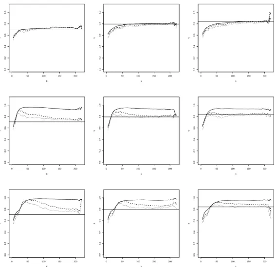
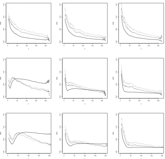
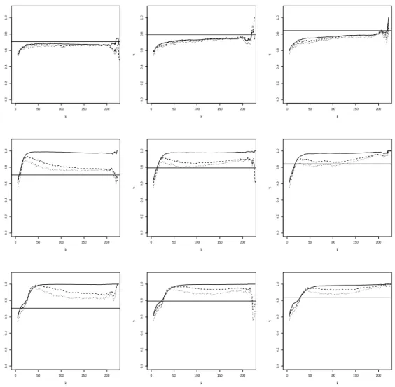
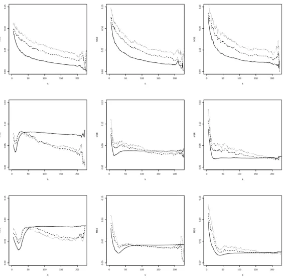
For each of the above distributions we simulate N “ 500 samples of size n “ 1 000. The results of the simulation experiment are reported in Figures 1 till 6. In Figure 1 we show the mean of ηqnpxq as a function of k for α “ 0 (solid line), α “ 0.5 (dashed line) and α “ 1 (dotted line) for the BB6 copula. The true value of η is represented by the horizontal reference line. The columns of the figure represent three different values of x, while the rows correspond with the contamination percentages, 0%, 5% and 10% from top to bottom. Figure 2 displays the empirical mean squared error (MSE) as a function of k, but has otherwise a layout that is similar to Figure 1. Concerning the selection of hn and c, we note the following. In a first step

criterion. This implies that the range of k varies from one dataset to the other, so means and MSE’s would be based on a different number of observations when plotted as a function of k. In order to avoid this we take the median of the hnand c values obtained in the 500 simulations

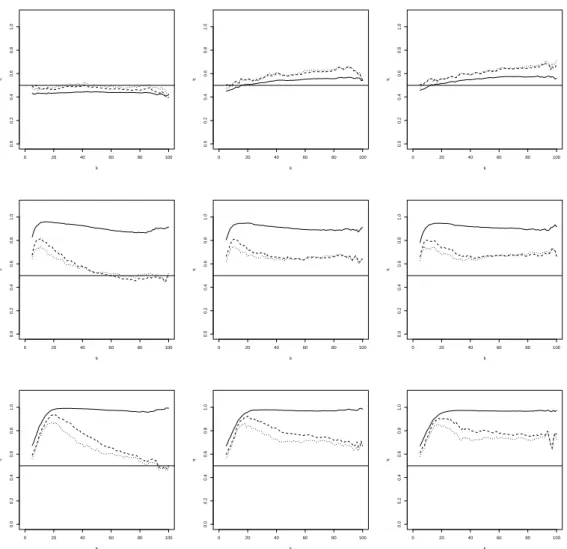
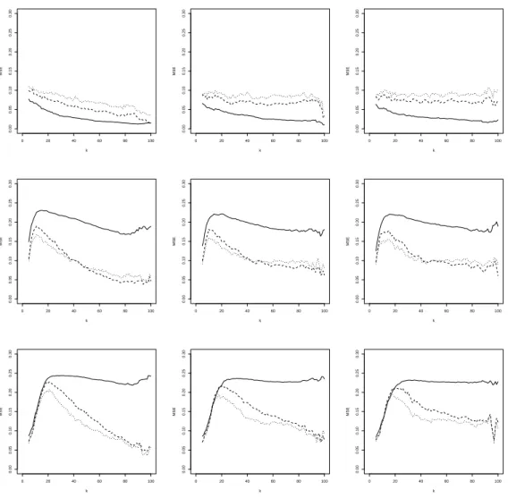
and use this for all estimations. Figures 3 and 4, and Figures 5 and 6, show the corresponding results for the Farlie Gumbel Morgenstern and BB9 copula, respectively. From the simulation we can draw the following conclusions:

• In absence of contamination, the estimators show generally a quite stable pattern for a wide range of k, close to the true value of η, despite the mis-specification of the parameter ρ. In terms of MSE we see that, the estimator with α “ 0, which corresponds to maximum likelihood, performs best, followed by α “ 0.5 and α “ 1. This can be explained as follows: in terms of bias the estimators with different values of α perform similarly, while for the variance we have that α “ 0, corresponding to maximum likelihood, performs best. It is well-known that the efficiency of the MDPDE decreases with increasing α, see, e.g., Basu et al. (1998).

• When there is contamination, then the non-robust estimator pα “ 0q is clearly affected, with a sample mean that can be far from the true value, while the robust estimators generally stay closer to the true value. The estimator with α “ 1, which offers the highest robustness, performs best in terms of bias. In terms of minimal MSE, using α “ 0.5 gives the best result. The advantage of α “ 1 in terms of bias is offset by its increased variance compared to α “ 0.5.

• The performance of the estimators deteriorates under increasing contamination percent-ages.

• For the BB6 distribution, the effect of the contamination is strongest for the smaller x values. This could be expected, as the dependence in the data is weakest at the smaller x. The dependence increases with x, and therefore at x “ 4 the effect of contamination on the diagonal is least.

• The Farlie Gumbel Morgenstern distribution has η “ 0.5, corresponding to near indepen-dence. For this distribution, contamination on the diagonal is clearly very severe.

• For the BB9 distribution, which does not satisfy our model assumptions, we still have very good estimation results, which also illustrates the robustness of our methodology with respect to violation of the model assumption. Also here we see that the effect of the contamination is biggest at the x positions where the dependence in the data is weakest. • Overall, using α “ 0.5 and 1 leads to estimators that are robust with respect to outliers. In

terms of minimal MSE the estimator with α “ 0.5 performs typically best, and is therefore the recommended value. This is in line with the findings of Dutang et al. (2014) in the context without covariates.

0 50 100 150 200 0.0 0.2 0.4 0.6 0.8 1.0 k η 0 50 100 150 200 0.0 0.2 0.4 0.6 0.8 1.0 k η 0 50 100 150 200 0.0 0.2 0.4 0.6 0.8 1.0 k η 0 50 100 150 200 0.0 0.2 0.4 0.6 0.8 1.0 k η 0 50 100 150 200 0.0 0.2 0.4 0.6 0.8 1.0 k η 0 50 100 150 200 0.0 0.2 0.4 0.6 0.8 1.0 k η 0 50 100 150 200 0.0 0.2 0.4 0.6 0.8 1.0 k η 0 50 100 150 200 0.0 0.2 0.4 0.6 0.8 1.0 k η 0 50 100 150 200 0.0 0.2 0.4 0.6 0.8 1.0 k η

Figure 1: BB6 simulation with (shifted) diagonal contamination. Mean of ηqnpxq with α “ 0 (solid line), α “ 0.5 (dashed line) and α “ 1 (dotted line), as a function of k at x “ 2 (left), x “ 3 (middle) and x “ 4 (right). From top to bottom: 0%, 5% and 10% of contamination.

5

A real data analysis

In this section, the proposed methodology is applied to a dataset of air pollution measurements. In environmental science, one needs to consider simultaneous high levels of several pollutants, possibly combined with high temperatures, as these may pose a major threat to human health. Estimation of the extreme dependence is thus of crucial importance in this context. We consider the data collected by the United States Environmental Protection Agency (EPA), publicly avail-able at https:{{aqsdr1.epa.gov{aqsweb{aqstmp{airdata{download files.html. The dataset under consideration contains monthly maxima on, among others, temperature, and ground-level ozone,

0 50 100 150 200 0.00 0.05 0.10 0.15 k MSE 0 50 100 150 200 0.00 0.05 0.10 0.15 k MSE 0 50 100 150 200 0.00 0.05 0.10 0.15 k MSE 0 50 100 150 200 0.00 0.05 0.10 0.15 k MSE 0 50 100 150 200 0.00 0.05 0.10 0.15 k MSE 0 50 100 150 200 0.00 0.05 0.10 0.15 k MSE 0 50 100 150 200 0.00 0.05 0.10 0.15 k MSE 0 50 100 150 200 0.00 0.05 0.10 0.15 k MSE 0 50 100 150 200 0.00 0.05 0.10 0.15 k MSE

Figure 2: BB6 simulation with (shifted) diagonal contamination. MSE of ηqnpxq with α “ 0 (solid line), α “ 0.5 (dashed line) and α “ 1 (dotted line), as a function of k at x “ 2 (left), x “ 3 (middle) and x “ 4 (right). From top to bottom: 0%, 5% and 10% of contamination.

carbon monoxide and particulate matter concentrations, for the time period 1999 to 2013. These data are collected at stations spread over the U.S. We will estimate the extreme dependence between ground-level ozone and particulate matter concentrations, conditional on the covariates time and location, where the latter is expressed by latitude and longitude. The method is imple-mented with the same cross-validation criteria as in the simulations, though for convenience we rescaled each covariate to the interval r0, 1s. As for the kernel function, we used the bi-quadratic kernel, generalised to the case p “ 3, as follows

Khnpxq “ 1 h3 n K ˆ }x} hn ˙ ,

0 20 40 60 80 100 0.0 0.2 0.4 0.6 0.8 1.0 k η 0 20 40 60 80 100 0.0 0.2 0.4 0.6 0.8 1.0 k η 0 20 40 60 80 100 0.0 0.2 0.4 0.6 0.8 1.0 k η 0 20 40 60 80 100 0.0 0.2 0.4 0.6 0.8 1.0 k η 0 20 40 60 80 100 0.0 0.2 0.4 0.6 0.8 1.0 k η 0 20 40 60 80 100 0.0 0.2 0.4 0.6 0.8 1.0 k η 0 20 40 60 80 100 0.0 0.2 0.4 0.6 0.8 1.0 k η 0 20 40 60 80 100 0.0 0.2 0.4 0.6 0.8 1.0 k η 0 20 40 60 80 100 0.0 0.2 0.4 0.6 0.8 1.0 k η

Figure 3: FGM simulation with (shifted) diagonal contamination. Mean of ηqnpxq with α “ 0 (solid line), α “ 0.5 (dashed line) and α “ 1 (dotted line), as a function of k at x “ ´0.5 (left), x “ 0.5 (middle) and x “ 0.8 (right). From top to bottom: 0%, 5% and 10% of contamination.

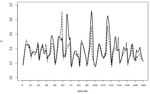
where x P R3, and }.} denotes the Euclidean norm. In Figure 7, we show the estimate of ηpxq with α “ 0 (solid line), α “ 0.5 (dashed line) and α “ 1 (dotted line) for the city of Los Angeles at different points in time. The reported estimate is medianpηqnpxq; k “ n

˚

{2, . . . , n˚´ 1q, where n˚ _{denotes the number of observations in Bpx, h}

nq. Overall, the extreme dependence between

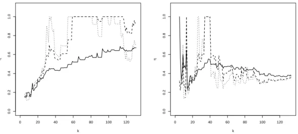
ground-level ozone and particulate matter concentrations shows a seasonal pattern, where the dependence is stronger in summer than winter. For some months the estimate with α “ 0 differs noticeably from those obtained with α “ 0.5 and α “ 1, which indicates the presence of observations that are disturbing for the estimation of the dependence structure. In Figure 8, we show the estimate ηqnpxq with α “ 0 (solid line), α “ 0.5 (dashed line) and α “ 1 (dotted line)

0 20 40 60 80 100 0.00 0.05 0.10 0.15 0.20 0.25 0.30 k MSE 0 20 40 60 80 100 0.00 0.05 0.10 0.15 0.20 0.25 0.30 k MSE 0 20 40 60 80 100 0.00 0.05 0.10 0.15 0.20 0.25 0.30 k MSE 0 20 40 60 80 100 0.00 0.05 0.10 0.15 0.20 0.25 0.30 k MSE 0 20 40 60 80 100 0.00 0.05 0.10 0.15 0.20 0.25 0.30 k MSE 0 20 40 60 80 100 0.00 0.05 0.10 0.15 0.20 0.25 0.30 k MSE 0 20 40 60 80 100 0.00 0.05 0.10 0.15 0.20 0.25 0.30 k MSE 0 20 40 60 80 100 0.00 0.05 0.10 0.15 0.20 0.25 0.30 k MSE 0 20 40 60 80 100 0.00 0.05 0.10 0.15 0.20 0.25 0.30 k MSE

Figure 4: FGM simulation with (shifted) diagonal contamination. MSE of ηqnpxq with α “ 0 (solid line), α “ 0.5 (dashed line) and α “ 1 (dotted line), as a function of k at x “ ´0.5 (left), x “ 0.5 (middle) and x “ 0.8 (right). From top to bottom: 0%, 5% and 10% of contamination.

for months 59 and 100 as a function of k. For month 59, the robust estimates show a stable pattern around ηpxq “ 1 for the second half of the k range, while the non-robust estimate shows nearly no stability as a function of k. On the contrary, for month 100, the robust estimates are below the non-robust estimate. Again the robust estimates show a stable horizontal pattern for the second half of the k range, which is not present for the non-robust estimate.

0 50 100 150 200 0.0 0.2 0.4 0.6 0.8 1.0 k η 0 50 100 150 200 0.0 0.2 0.4 0.6 0.8 1.0 k η 0 50 100 150 200 0.0 0.2 0.4 0.6 0.8 1.0 k η 0 50 100 150 200 0.0 0.2 0.4 0.6 0.8 1.0 k η 0 50 100 150 200 0.0 0.2 0.4 0.6 0.8 1.0 k η 0 50 100 150 200 0.0 0.2 0.4 0.6 0.8 1.0 k η 0 50 100 150 200 0.0 0.2 0.4 0.6 0.8 1.0 k η 0 50 100 150 200 0.0 0.2 0.4 0.6 0.8 1.0 k η 0 50 100 150 200 0.0 0.2 0.4 0.6 0.8 1.0 k η

Figure 5: BB9 simulation with (shifted) diagonal contamination. Mean of ηqnpxq with α “ 0 (solid line), α “ 0.5 (dashed line) and α “ 1 (dotted line), as a function of k at x “ 2 (left), x “ 3 (middle) and x “ 4 (right). From top to bottom: 0%, 5% and 10% of contamination.

6

Appendix

6.1 Proof of Theorem 2.1

The first step consists to show that, under our assumptions, ErTnpK, s, j|xqs “ fXpxqFZpun|xqη0jpxqj! ˆ " 1 p1 ´ sη0pxqqj`1 ´δZpun|xq η0pxq „ 1 p1 ´ sη0pxqqj`1 ´ 1 ´ ρ0pxq p1 ´ ρ0pxq ´ sη0pxqqj`1  ` opδZpun|xqq `O ´ hδnfX^δC ¯ ` O ´ hδη n ln un ¯) ,

0 50 100 150 200 0.00 0.05 0.10 0.15 k MSE 0 50 100 150 200 0.00 0.05 0.10 0.15 k MSE 0 50 100 150 200 0.00 0.05 0.10 0.15 k MSE 0 50 100 150 200 0.00 0.05 0.10 0.15 k MSE 0 50 100 150 200 0.00 0.05 0.10 0.15 k MSE 0 50 100 150 200 0.00 0.05 0.10 0.15 k MSE 0 50 100 150 200 0.00 0.05 0.10 0.15 k MSE 0 50 100 150 200 0.00 0.05 0.10 0.15 k MSE 0 50 100 150 200 0.00 0.05 0.10 0.15 k MSE

Figure 6: BB9 simulation with (shifted) diagonal contamination. MSE of ηqnpxq with α “ 0 (solid line), α “ 0.5 (dashed line) and α “ 1 (dotted line), as a function of k at x “ 2 (left), x “ 3 (middle) and x “ 4 (right). From top to bottom: 0%, 5% and 10% of contamination.

0.0 0.2 0.4 0.6 0.8 1.0 Month η 0 12 24 36 48 60 72 84 96 108 120 132 144 156 168 180

Figure 7: Air pollution data. Time plot ofηqnpxq with α “ 0 (solid line), α “ 0.5 (dashed line) and α “ 1 (dotted line) for the city of Los Angeles.

To obtain this result for the case j ą 0, use the following decomposition ErTnpK, s, j|xqs “ fXpxq ż8 1 ppzqFZpunz|xqdz ` ż SK Kpvq ż8 1 ppzqFZpunz|xqdzrfXpx ´ hnvq ´ fXpxqsdv `fXpxq ż SK Kpvq ż8 1 ppzqrFZpunz|x ´ hnvq ´ FZpunz|xqsdz dv ` ż SK Kpvq ż8 1 ppzqrFZpunz|x ´ hnvq ´ FZpunz|xqsdz rfXpx ´ hnvq ´ fXpxqsdv,

where ppzq :“ szs´1pln zqj ` jzs´1pln zqj´1. Each term can be treated using our H¨older-type conditions, which imply in particular that, for n large enough, z ě un, and some constants

M1, M2, M3 ˇ ˇ ˇ ˇ FZpz|x ´ hnvq FZpz|xq ´ 1 ˇ ˇ ˇ ˇď M1 ´ hδC n ` zM2h δη n <sub>h</sub>δη n ln z ` |δZpz|xq|hδnA` |δZpz|xq|zM3h δε n _hδε n ln z ¯ (12) combined with a slight modification of Proposition 2.3 in Beirlant et al. (2009) which ensures

0 20 40 60 80 100 120 0.0 0.2 0.4 0.6 0.8 1.0 k η 0 20 40 60 80 100 120 0.0 0.2 0.4 0.6 0.8 1.0 k η

Figure 8: Air pollution data. ηqnpxq with α “ 0 (solid line), α “ 0.5 (dashed line) and α “ 1 (dotted line) as a function of k for months 59 (left) and 100 (right).

that sup zě1 z 1 ηpxq ˇ ˇ ˇ ˇ FZpunz|xq FZpun|xq ´ Gpz; ηpxq, δZpun|xq, ρpxqq ˇ ˇ ˇ ˇ“ op|δZpun|xq|q as unÑ 8. In case j “ 0 we obtain ErTnpK, s, 0|xqs “ ż SK Kpvq ż8 1 ppzqFZpunz|x ´ hnvqdzfXpx ´ hnvqdv ` ż SK KpvqFZpun|x ´ hnvqfXpx ´ hnvqdv,

where ppzq “ szs´1. Both terms can be analysed with decompositions similar to the ones used for the case j ą 0.

Then we can follow the lines of proofs of Theorem 1 and Corollary 1 in Dierckx et al. (2014) in order to achieve the proof of Theorem 2.1.

6.2 Proof of Theorem 3.1

d nhpn FZpun|xqfXpxq ” q TnpK, s, j|xq ´ TnpK, s, j|xq ı “ d nhpn FZpun|xqfXpxq ” q TnpK, s, j|xq ´ TnpK, s, j|xq ´ E ´ q TnpK, s, j|xq ´ TnpK, s, j|xq ¯ı ` d nhpn FZpun|xqfXpxq E ´ q TnpK, s, j|xq ´ TnpK, s, j|xq ¯ “: Rn,1` Rn,2.

We will study the two terms Rn,1and Rn,2separately. First, we start with the term Rn,1. Define

for any s ă 0 with j P J :“ t0, 1, 2, 3u or ps, jq “ p0, 0q

gps,jq_ξ,n py1, y2, vq :“ d hpn FZpun|xqfXpxq Khnpx ´ vqq ps,jq ξ,n py1, y2, vq with q_ξ,nps,jqpy1, y2, vq :“ ˆ Z_ξpy1, y2, vq un ˙sˆ lnZξpy1, y2, vq un ˙j 1ltZξpy1,y2,vqąunu, Zξpy1, y2, vq :“ min ˆ 1 |1 ´ ξ1py1, y2, vq| , 1 |1 ´ ξ2py1, y2, vq| ˙ , and measurable ξ P H :“ tξ “ pξ1, ξ2q; ξ : R ˆ R ˆ SX Ñ R2u.

For convenience, denote ξn“ pFn,1, Fn,2q and ξ0 “ pF1, F2q. According to Lemma 3.1, r´1n |ξn´ξ0|

converges in probability towards the null function H0 “ t0u in H, endowed with the norm

}ξ}H :“ }ξ1}8` }ξ2}8 for any ξ P H. Consider now the class

Eps,jq n pbq :“ tg ps,jq ξ0`rnξ,n´ g ps,jq ξ0,n : ξ P H, }ξ}H ď bu,

with envelope function Gps,jqn pbq. Our aim is to apply Theorem 2.3 in van der Vaart and Wellner

(2017). To reach this goal, we need to introduce some notations. Let P denote the law of the vector pYp1q_{, Y}p2q_{, Xq and define the expectation of any real-valued measurable function f under}

P by P f “ş fdP .

We have now to show the two following results:

Assertion 1: For any s ă 0 with j P J or ps, jq “ p0, 0q, we have ?

nP Gps,jq

n pbnq ÝÑ 0 for all bnÑ 0,

and

Assertion 2: For any s ă 0 with j P J or ps, jq “ p0, 0q, we have P

´

pGps,jq_n pbqq2 ¯

6.2.1 Proof of Assertion 1

We start to consider the case where s ă 0 with j P J . As a first step we derive an envelope function for Enps,jqpbnq. We have

ˇ ˇ ˇq ps,jq ξ0`rnξ,n´ q ps,jq ξ0,n ˇ ˇ ˇ “ ˇ ˇ ˇ ˇ ż8 1

ppaq1l_tunăunaăZ_{ξ0`rnξ</sub>u1ltZ<sub>ξ0`rnξ}ąunuda ´

ż8

1

ppaq1l_tunăunaăZ_ξ0u1ltZ_ξ0ąunuda

`1ltj“0u1ltZ<sub>ξ0`rnξ</sub>ąunu´ 1ltj“0u1ltZ_ξ0ąunu

ˇ ˇ ˇ ď ż8 1 |ppaq| ˇ ˇ

ˇ1ltunăunaăZ_{ξ0`rnξ</sub>u1ltZ<sub>ξ0`rnξ}ąunu´ 1ltunăunaăZ_ξ0u1ltZ_ξ0ąunu

ˇ ˇ ˇ da `1ltj“0u ˇ ˇ ˇ1ltZ<sub>ξ0`rnξ</sub>ąunu´ 1ltZ_ξ0ąunu ˇ ˇ ˇ ď ż8 1 |ppaq| ˇ ˇ

ˇ1ltunăunaăZ_ξ0u´ 1ltunăunaăZ_ξ0`rnξu

ˇ ˇ ˇ 1ltZ_ξ0ąunuda ` ż8 1

|ppaq| 1ltunăunaăZ_ξ0`rnξu

ˇ ˇ ˇ1ltZ<sub>ξ0`rnξ</sub>ąunu´ 1ltZ<sub>ξ0</sub>ąunu ˇ ˇ ˇ da `1ltj“0u ˇ ˇ ˇ1ltZ_ξ0`rnξąunu´ 1ltZ_ξ0ąunu ˇ ˇ ˇ ď ż8 1

|ppaq| 1ltminpZ_ξ0,Z_{ξ0`rnξ</sub>qďunaďmaxpZ<sub>ξ0</sub>,Z<sub>ξ0`rnξ}qu1ltZ_ξ0ąunuda

` ż8

1

|ppaq| 1ltunăunaăZ_{ξ0`rnξ</sub>u1ltminpZ<sub>ξ0</sub>,Z<sub>ξ0`rnξ}qďunďmaxpZ_ξ0,Z_ξ0`rnξquda

`1ltj“0u1ltminpZ<sub>ξ0</sub>,Z<sub>ξ0`rnξ</sub>qďunďmaxpZ_ξ0,Z_ξ0`rnξqu. (13)

tuna P rminpZξ0, Zξ0`rnξq; maxpZξ0, Zξ0`rnξqsu “ " una P „ min ˆ min ˆ 1 |1 ´ F1´ rnξ1| , 1 |1 ´ F2´ rnξ2| ˙ , min ˆ 1 1 ´ F1 , 1 1 ´ F2 ˙˙ ; max ˆ min ˆ 1 |1 ´ F1´ rnξ1| , 1 |1 ´ F2´ rnξ2| ˙ , min ˆ 1 1 ´ F1 , 1 1 ´ F2 ˙˙* “ " 1 una

P rmin pmax p|1 ´ F1´ rnξ1|, |1 ´ F2´ rnξ2|q , max p1 ´ F1, 1 ´ F2qq ;

max pmax p|1 ´ F1´ rnξ1|, |1 ´ F2´ rnξ2|q , max p1 ´ F1, 1 ´ F2qqsu

Ă " 1 una P rmin p|1 ´ F1´ rnξ1|, 1 ´ F1q , max p|1 ´ F1´ rnξ1|, 1 ´ F1qs * Y " 1 una P rmin p|1 ´ F2´ rnξ2|, 1 ´ F2q , max p|1 ´ F2´ rnξ2|, 1 ´ F2qs * Ă " 1 una P r1 ´ F1´ rnbn, 1 ´ F1` rnbns * Y " 1 una P r1 ´ F2´ rnbn, 1 ´ F2` rnbns * “: An,1paq Y An,2paq. (14) Also,

1ltZ_ξ0`rnξąunau “ 1lt|1´F1´rnξ1|ă_una1 ,|1´F2´rnξ2|ă_una1 u

ď 1l_t´ 1 una´rnbnă1´F1ă 1 una`rnbn,´ 1 una´rnbnă1´F2ă 1 una`rnbnu “ 1l_t1´F 1ă_una1 `rnbn,1´F2ă<sub>una</sub>1 `rnbnu,

and, taking into account that 1l_tZ ξ0ąunu “ 1lt1´F1ă_un1 ,1´F2ă_un1 u, we obtain 1ltZ<sub>ξ0`rnξ</sub>ąunau ď 1lt1´F1ă<sub>un</sub>1 p1<sub>a</sub>`rnunbnq,1´F2ă_un1 p1_a`rnunbnqu “ 1ltZ<sub>ξ0</sub>ą<sub>1</sub> un a `rnunbn u. (15)

Thus, combining (13), (14) and (15), we obtain the following envelope for Enps,jqpbnq:

Gps,jq_n pbnq :“ d hpn FZpun|xqfXpxq Khnpx ´ .q „ż8 1

|ppaq| 1ltAn,1paqYAn,2paqu1ltZ_ξ0ąunu da

` ż8 1 |ppaq| 1l" Z<sub>ξ0</sub>ą<sub>1</sub> un a `rnunbn *1l tAn,1p1qYAn,2p1qu da

with ? nP Gps,jq n pbnq “ d nhpn FZpun|xqfXpxq ˆ " E „ Khnpx ´ Xq ż8 1 |ppaq| E ´ 1l_{tAn,1paqYAn,2paqu}1l_tZ ξ0ąunu ˇ ˇ ˇX ¯ da  `E « Khnpx ´ Xq ż8 1 |ppaq| E ˜ 1l" Z<sub>ξ0</sub>ą<sub>1</sub> un a `rnunbn *1l tAn,1p1qYAn,2p1qu ˇ ˇ ˇ ˇ ˇ X ¸ da ff `1ltj“0uE « Khnpx ´ XqE ˜ 1l_{tAn,1p1qYAn,2p1qu} ˇ ˇ ˇ ˇ ˇ X ¸ff+ “ d nhpn FZpun|xqfXpxq ˆ "ż SK Kpvq ż8 1 |ppaq| E ´

1ltAn,1paqYAn,2paqu1ltZ_ξ0ąunu

ˇ ˇ ˇX “ x ´ hnv ¯ dafXpx ´ hnvqdv ` ż SK Kpvq ż8 1 |ppaq| E ˜ 1l" Z<sub>ξ0</sub>ą<sub>1</sub> un a `rnunbn *1l tAn,1p1qYAn,2p1qu ˇ ˇ ˇ ˇ ˇ X “ x ´ hnv ¸ dafXpx ´ hnvqdv `1ltj“0u ż SK KpvqE ´ 1l<sub>tAn,1p1qYAn,2p1qu</sub> ˇ ˇ ˇX “ x ´ hnv ¯ fXpx ´ hnvqdv * “: d nhpn FZpun|xqfXpxq tT1` T2` T3u .

Consider T1. By the Cauchy-Schwarz inequality

T1ď ż SK Kpvq ż8 1 |ppaq| b

PpAn,1paq Y An,2paq|X “ x ´ hnvqFZpun|x ´ hnvqdafXpx ´ hnvqdv.

The sub-additivity of probability measures and some straightforward calculations give then PpAn,1paq Y An,2paq|X “ x ´ hnvq ď PpAn,1paq|X “ x ´ hnvq ` PpAn,2paq|X “ x ´ hnvq

“ ż1 0 1l_t 1 un aPrz´rnbn,z`rnbnsudz ` ż1 0 1l_t 1 un aPrz´rnbn,z`rnbnsudz ď 2rnbn` 2rnbn“ 4rnbn. (17) Thus T1 ď 2 b rnbnFZpun|xq ż8 1 |ppaq| da ż SK Kpvq d FZpun|x ´ hnvq FZpun|xq fXpx ´ hnvqdv,

and hence, by (12) and the H¨older continuity of fX, we have T1“ O

ˆb

rnFZpun|xq

˙ .

As for T2 use again the Cauchy-Schwarz inequality and (17) to obtain T2 ď 2 a rnbn ż8 1 |ppaq| da ż SK Kpvq d FZ ˆ un 1 ` rnunbn ˇ ˇ ˇx ´ hnv ˙ fXpx ´ hnvqdv “ 2 d rnbnFZ ˆ un 1 ` rnunbn ˇ ˇ ˇx ˙ ż8 1 |ppaq| da ż SK Kpvq g f f f e FZ ´ un 1`rnunbn ˇ ˇ ˇx ´ hnv ¯ FZ ´ un 1`rnunbn ˇ ˇ ˇx ¯ fXpx ´ hnvqdv.

Note that under our assumptions, rnunÑ 0, as n Ñ 8. Thus using (12) and the fact that

FZ ´ un 1`rnunbn ˇ ˇ ˇx ¯ FZpun|xq Ñ 1, (18) we have that T2“ O ˆb rnFZpun|xq ˙ .

By similar arguments, we get T3 “ Oprnq “ o

ˆb

rnFZpun|xq

˙

under our assumptions (10) and (11).

Combining the above

? nP Gps,jq n pbnq “ O ´a nhpnrn ¯ .

Now, we move to the case ps, jq “ p0, 0q and use a similar proof. In that case, using (17), we have ? nP Gp0,0q_n pbnq “ d nhpn FZpun|xqfXpxq ż SK KpvqP ´ An,1p1q Y An,2p1q ˇ ˇ ˇX “ x ´ hnv ¯ fXpx ´ hnvqdv ď 4rnbn d nhpn FZpun|xqfXpxq ż SK KpvqfXpx ´ hnvqdv “ O ˜d nhpn FZpun|xq rnbn ¸ “ o´anhpnrn ¯

6.2.2 Proof of Assertion 2

Again, we start to look at the case s ă 0 and j P J . From (16) and straightforward bounds, we deduce that ´ Gps,jq_n pbq ¯2 ď h p n FZpun|xqfXpxq K_h2_npx ´ ¨q ˆ # ˆż8 1 |ppaq|da ˙ ż8 1 |ppaq|1l" Z_ξ0ą1 un a `rnunb *1l tAn,1p1qYAn,2p1quda `3 ˆż8 1 |ppaq|da ˙ ż8 1

|ppaq|1ltAn,1paqYAn,2paqu1ltZ_ξ0ąunuda

` ˆ 1 ` 4 ż8 1 |ppaq|da ˙ 1l_{tAn,1p1qYAn,2p1qu} * .

Since ş8₁ |ppaq|da ă 8, using again the Cauchy-Schwarz inequality combined with (17), we deduce that P ˆ ´ Gps,jq n pbq ¯2˙ ď C ? rn FZpun|xqfXpxq ż SK K2pvq ż8 1 |ppaq| g f f eF_Z ˜ un 1 a ` rnunb ˇ ˇ ˇ ˇ ˇ x ´ hnv ¸ da fXpx ´ hnvq dv ` C ? rn FZpun|xqfXpxq ż SK K2pvq ż8 1 |ppaq| b FZpun|x ´ hnvq da fXpx ´ hnvq dv ` Crn FZpun|xqfXpxq ż SK K2pvq fXpx ´ hnvq dv,

where C is a constant which can change from one line to each other. Finally, combining (12) with (18), we deduce that

P ˆ ´ Gps,jq_n pbq ¯2˙ “ O ˆc rn FZpun|xq ˙ . The case ps, jq “ p0, 0q can be dealt with similarly and leads to

P ˆ ´ Gp0,0q n pbq ¯2˙ “ O ˆ rn FZpun|xq ˙ . This achieves the proof of Assertion 2.

Combining Assertions 1 and 2 with Theorem 2.3 in van der Vaart and Wellner (2017) yields that Rn,1“ oPp1q.

Now, it remains to study the term Rn,2. To this aim, note that, for n large, |Rn,2| ď d nhpn FZpun|xqfXpxq E ˇ ˇ ˇTqnpK, s, j|xq ´ TnpK, s, j|xq ˇ ˇ ˇ ď ?nE ˇ ˇ ˇg ps,jq ξn,npY p1q_{, Y}p2q_{, Xq ´ g}ps,jq ξ0,npY p1q_{, Y}p2q_{, Xq}ˇˇ ˇ ď ?nP Gps,jq n pbq,

since ξnP ξ0` rnBp0, bq where Bp0, bq :“ tξ : }ξ}H ď bu (where we use the Skorohod

represen-tation). According to the proof of Assertion 1, since bnÑ 0 can be replaced by any fixed value

b without changing the conclusion, we have Rn,2“ op1q.

Combining the results for Rn,1 and Rn,2 achieves the proof of Theorem 3.1.

References

Barbe, P., Foug`eres, A.-L. and Genest, C. (2006). On the tail behavior of sums of dependent risks. Astin Bull., 36, 361–373.

Basu, A., Harris, I.R., Hjort, N.L. and Jones, M.C. (1998). Robust and efficient estimation by minimizing a density power divergence. Biometrika, 85, 549–559.

Beirlant, J., Dierckx, G., Goegebeur, Y. and Matthys, G. (1999). Tail index estimation and an exponential regression model. Extremes, 2, 177–200.

Beirlant, J., Dierckx, G. and Guillou, A. (2011). Bias-reduced estimators for bivariate tail mod-elling. Insurance Math. Econom., 49, 18–26.

Beirlant, J., Goegebeur, Y., Segers, J. and Teugels, J. (2004). Statistics of Extremes – Theory and Applications. Wiley.

Beirlant, J., Joossens, E. and Segers, J. (2009). Second-order refined peaks-over-threshold mod-elling for heavy-tailed distributions. J. Statist. Plann. Inference, 139, 2800–2815.

Daouia, A., Gardes, L. and Girard, S. (2013). On kernel smoothing for extremal quantile regres-sion. Bernoulli, 19, 2557–2589.

Daouia, A., Gardes, L., Girard, S. and Lekina, A. (2011). Kernel estimators of extreme level curves. TEST, 20, 311–333.

Dierckx, G., Goegebeur, Y. and Guillou, A. (2014). Local robust and asymptotically unbiased estimation of conditional Pareto type-tails. TEST, 23, 330–355.

Draisma, G., Drees, H., Ferreira, A. and de Haan, L., (2004). Bivariate tail estimation: depen-dence in asymptotic independepen-dence. Bernoulli, 10, 251–280.

Dutang, C., Goegebeur, Y. and Guillou, A. (2014). Robust and unbiased estimation of the coefficient of tail dependence. Insurance Math. Econom., 57, 46–57.

Escobar-Bach, M., Goegebeur, Y. and Guillou, A. (2018). Local robust estimation of the Pickands dependence function. Ann. Statist., 46, 2806–2843.

Feuerverger, A. and Hall, P. (1999). Estimating a tail exponent by modelling departure from a Pareto distribution. Ann. Statist., 27, 760–781.

Gin´e, E. and Guillou, A. (2002). Rates of strong uniform consistency for multivariate kernel density estimators. Ann. Inst. Henri Poincar´e Probab. Stat., 38, 907–921.

Gin´e, E., Koltchinskii, V. and Zinn, J. (2004). Weighted uniform consistency of kernel density estimators. Ann. Probab., 32, 2570–2605.

Goegebeur, Y. and Guillou, A. (2013). Asymptotically unbiased estimation of the coefficient of tail dependence. Scand. J. Stat., 40, 174–189.

Gomes, M.I. and Martins, M.J. (2004). Bias reduction and explicit estimation of the extreme value index. J. Statist. Plann. Inference, 124, 361–378.

de Haan, L. and Ferreira, A. (2006). Extreme Value Theory: An Introduction. Springer. Joe, H. (1997). Multivariate models and dependence concepts. Chapman and Hall, London. Ledford, A.W. and Tawn, J.A. (1997). Modelling dependence within joint tail regions. J. Roy.

Statist. Soc. Ser. B, 59, 475–499.

Peng, L. (1999). Estimation of the coefficient of tail dependence in bivariate extremes. Statist. Probab. Lett., 43, 399–409.

van der Vaart, A. W. and Wellner, J. A. (2007). Empirical processes indexed by estimated func-tions, Asymptotics: Particles, Processes and Inverse Problems, IMS Lecture Notes Monogr. Ser., 55, 234–252.

Yao, Q. (1999). Conditional predictive regions for stochastic processes. Technical report, Uni-versity of Kent at Canterbury.