Numerical simulation of wave propagation in the Grenoble basin: Benchmark ESG2006

HAL Id: hal-00714032

https://hal-brgm.archives-ouvertes.fr/hal-00714032

HAL is a multi-disciplinary open access archive for the deposit and dissemination of sci-entific research documents, whether they are pub-lished or not. The documents may come from teaching and research institutions in France or abroad, or from public or private research centers.

L’archive ouverte pluridisciplinaire HAL, est destinée au dépôt et à la diffusion de documents scientifiques de niveau recherche, publiés ou non, émanant des établissements d’enseignement et de recherche français ou étrangers, des laboratoires publics ou privés.

Hideo Aochi, Julien Rey, John Douglas

To cite this version:

Hideo Aochi, Julien Rey, John Douglas. Numerical simulation of wave propagation in the Grenoble basin: Benchmark ESG2006. Third International Symposium on the Effects of Surface Geology on Seismic Motion, Aug 2006, Grenoble, France. Paper Number: 32. �hal-00714032�

Third International Symposium on the Effects of Surface Geology on Seismic Motion Grenoble, France, 30 August - 1 September 2006

Paper Number: 32

NUMERICAL SIMULATION OF WAVE PROPOGATION IN THE

GRENOBLE BASIN: BENCHMARK ESG2006

Hideo AOCHI1, Julien REY1, John DOUGLAS1

1 BRGM – ARN/RIS, Orléans, France

ABSTRACT - Numerical simulations of wave propagation in the Grenoble basin are undertaken using the finite difference method (FDM) in a staggered grid framework (4th order in space) for an elastic medium with a flat ground surface and perfectly matching layer absorbing boundaries. The seismic source is introduced in the form of a seismic moment tensor irrespective of whether a point source or expanding finite source model is used. This is the same methodology adopted in our previous studies (Aochi and Douglas, 2006; Douglas et al., 2006). As the FD grids in our code are equally spaced in both horizontal and vertical directions, the grid size should be fine enough to describe the Grenoble Basin where a low velocity (300m/s) zone is present near the surface (a few 100 m depth at maximum) while the surrounding bedrock has a velocity ten times higher. We carry out the simulations with different resolutions (a grid size of 100 m and of 50 m). Both of them require high performance computation resources.

This benchmark test is an interesting application for seismic hazard evaluation because of the high contrast basin structure and its non-negligible dimensions. For the two large earthquake scenarios (S1 and S2 of magnitude 6), our numerical simulations are compared with empirical ground-motion models for peak ground velocity (PGV) to validate the calculations and to evaluate the local effect of the Grenoble basin. The equations derived by Campbell (1997) better match the simulations for the rock sites outside the basin than for the soil sites within the basin. It is remarkable that PGVs at some basin sites show changes of several times at the same distance from the earthquake fault. We also observe strong directivity effects from rupture propagation along the fault. The obtained scatter is compatible with other simulations which we have performed recently using dynamic rupture models and different crust structure models (Aochi & Douglas, 2006; Douglas et al., 2006). As the resolution of the basin model is not enough good and the inelastic attenuation is not fully taken into account, it is still difficult to quantitatively compare signal durations. However it is visible that the basin resonates a long time after the passage of body waves.

1. Introduction

This article presents the ground motions computed for the three earthquake scenarios of the ESG2006 benchmark on ground motion simulation. First simulations from two small real earthquakes (M 2.8-2.9, named W1 and W2) are compared with the velocity time-histories observed at three different stations. The other two scenarios consist of hypothetical pure strike-slip earthquakes of Mw 6.0, occurring close to the Grenoble

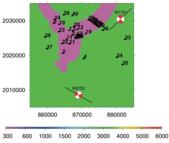
sediment-filled valley, named S1 and S2, whose hypocenters are the same as W1 and W2 respectively. Ground velocities at 40 (9 on rock and 31 within the valley) stations are discussed (Figure 1).

The first section of this paper briefly introduces the simulation method used, both in terms of the kinematic rupture model adopted and the computation method used for wave propagation. The following section presents the simulated ground velocities for the four scenarios. In particular, comparisons are made between the simulated PGV and those predicted by recent empirical ground motion estimation equations.

Figure 1. 2D map (S-wave velocity on the ground surface) simulated in this study. Map scale is in meters.

2. Simulation method

For the simulations here the following simulation scheme was used, which is a similar scheme to that used by Douglas et al. (2006) to model ground motions in three French regions. A standard equally spaced staggered finite difference method (FDM), which is fourth order in space and second order in time (Levander, 1988, Olsen, 1994), is used. Our code was previously used for testing dynamic rupture propagation and the consequent wave propagation along finite segmented faults for the 1999 Izmit earthquake (Aochi & Madariaga, 2003). Other aspects of this type of FDM are detailed in Graves (1996). Furthermore, our procedure is characterised by the implementation of a finite fault model (Olsen et al., 1999) and the PML absorbing condition (Collino & Tsogka, 2001). The lower depth of the basin shape is given within a file at every 250m. In our simulation, we linearly interpolate it where necessary. We truncate the northern end of the given model by a few km to improve calculating efficiency. Our modelling volume is then 30km x 30 km x 10 km. The medium heterogeneity is averaged in the manner of Graves (1996). The qualify factor of the attenuation Q is taken as infinity in the bedrock and 50 within the basin. The station location is approximated at one of the closest FD grid points after converting the given WGS coordinates into geographical Lambert coordinates. As in Figure 1, our model globally conforms to the true situation, but in detail, for example, station 1 is located on the bedrock in the field but is on sediment in the simulation. Though station 8 (541.5 m depth) is located correctly in the bedrock medium, the lower depth of the basin is embedded at around 480-500 m depth in our simulations. The output at this station is strongly affected by this medium boundary. The border area of the strong contrast in the medium is not suitable for quantitative comparison because of the

numerical treatment in the program as well as the inherent numerical instability of the FDM.

Due to the strong contrast of the basin sediment and its non-negligible dimension, it is necessary to calculate with a fine grid spacing. Preliminary simulations are carried out using a grid of 100 m (time step 0.005 sec), with which our regional scale simulations are often executed. However, our target earthquakes generally have a magnitude of more than 4 and the assumed slowest S-wave velocity is around 1000 – 2000 m/s, that is, the usual target is a few Hz at rock sites. Finer simulations with a grid of 50 m (time step 0.003) are tested here with help of our Computational System and Technology division (STI). This size is required by a simple analogy of the need of 5 grid points for a target wavelength (1 Hz wave for Vs=300m/s and the thickness of sediment layer of a few hundred meters). This may allow observation up to 1 Hz in the basin (on the sediment) and 10 Hz at rock sites at best. Through a brief study, the waveforms calculated with different resolutions are similar at rock sites. The early phase of waveforms at sediment sites seems similar, while the significant differences appear in later phases (resonance of the basin). However, even with these finer simulations, it is difficult to physically discuss those later phases, because the given structure model and the grids may not be sufficient and because the method of wave attenuation is too simple.

Concerning the seismic sources used as input, we use a locally supported B-spline function of order 4 (degree 3) for describing a smoothed piece-like function instead of the differential error function. It is an advantage that the B-spline function has a local support (finite duration) so that the origin time is always zero in our simulations. When this function is used as a source time function of a point source, it is known that the frequency context is not the one expected (i.e. flat at low frequencies in acceleration) (Douglas et al., 2006). However this is sufficient to discuss the wave form in the time domain such as PGV, if we choose a reasonable duration according to the magnitude. When this is used as a slip function in a finite fault model, the form of the function becomes less important than the other factors such as rupture velocity, directivity, dimension etc. One has to introduce a complex asymmetric function for the slip history for more realistic simulations. In any case, in our simulation, we do not introduce any further factors generating complexity in the waveforms. Some further remarks should be added. Though a rise time of 0.03 s is required for the small earthquakes, but it is in fact too short to realise because it may lead to unnecessary numerical oscillations. We limit the rise time to 0.2 s (5 Hz) for the tests. The simulation results are comparable not with the amplitudes and frequency contents of the observations but with the arrival times and with relative comparisons among different stations. For the large earthquakes, the proposed values of a rise time of 1.116 s, a uniform final slip of 1.116 m and a rupture velocity of 2.8 km/s as well as the given fault location and dimension are followed except for the mechanism of S2 (which was originally stated to be right lateral faulting).

3. Results

This section presents the results obtained for the 4 scenarios (W1, W2, S1 and S2), which are compared with the observed ground motions at the given stations, within the simulations with different numerical procedures and with empirical equations.

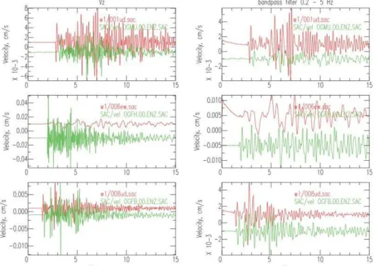
Figure 2 compares the simulated ground velocities for the seismic source W1 at the stations 1, 6 and 8, which correspond to OGMU, OGFH and OGFB, respectively. This simulation is carried out with a grid of 100 m, which is not fine enough for wave propagation within the basin. In the simulation, station 8 is just located on bedrock (the output is sampled at a depth of 600m) like the corresponding station OGFB so both should be comparable. Characteristic waveforms are commonly observed, but the arrivals are systematically shifted (they are earlier in the simulation). This may be because the event time or location and/or the medium properties are not well constrained, unless the problem is due to numerical problems. Station 6 shows the surface ground motion at the same location. The waveforms are not similar because of the lack of resolution. We recall again that station 1 is located on sediments in the simulation unlike the corresponding station OGMU. The

Figure 2. Simulated (red) and observed (green) ground velocities for W1.

3.2 Duration of event (W2: Mw 2.8)

Figure 3 compares the ground motion at three different stations on rock between two simulations for the seismic source W2. One of the simulation uses a rise time of 0.2 s as in all the other simulations, while the other adopted 0.003 s as proposed. Briefly it may be estimated that the resolution is up to 5 Hz at most with respect to wave propagation in the bedrock (Vs of about 3000 m/s, grid size of 100m). As clearly observed, there are very strong spikes after the arrivals of body waves in the raw output (left column). They must be from inevitable numerical disturbances within the FDM because they do not disappear until the application of a filter with a cut off up to 5 Hz. In this case, the information on the high frequency generation (source duration shorter than this period) is lost and the obtained synthetic waveforms become identical. It leads to the conclusion that short period behaviors of the seismic source become unimportant when compare with the numerical resolution of the FDM.

Figure 3. Comparison of ground motions at stations on bedrock for the seismic source W1 using different event durations: 0.2 s in red, and 0.03 in green.

3.3 Large event (S1: Mw 6.0)

Figure 4 shows the simulated ground velocity for six different stations for the seismic source S1 from two simulations using different grid sizes. As expected, both waveforms are similar for the rock sites (numerical resolution is sufficient). From the waveforms at these rock sites, it can be seen that the rupture process is very simple without any complexity regardless of its finite dimension. On the other hand, within the basin on the sediments, the early phases seem to be similar in both simulations, but the later phases differ especially for stations in the near field and in the horizontal direction due to a lack of resolution. It confirms that high resolution should be required for discussing the ground motions in the basin. In general, the simulations well reproduce the amplification and long shaking duration in the basin. The same tendency is observed in the simulations obtained for the source S2.

Figure 4. Simulated ground velocities with different grid sizes: 100m (red) and 50m (green) at six different stations. The left two columns are for stations on bedrock and the right two columns are

for stations in the basin (on sediment).

3.4 Comparison to empirical ground-motion estimates

Similarly to the approach adopted by Aochi & Douglas (2006), the predicted ground motions from the M6.0 earthquakes (S1 and S2) are compared to empirical ground-motion models for the estimation of PGV. These five recent equations for the estimation of PGV from shallow crustal earthquakes have been selected: Campbell (1997), Sadigh & Egan (1998), Chapman (1999), Tromans & Bommer (2002) and Pankow & Pechmann (2004). For the equation of Tromans & Bommer (2002), which uses surface-wave magnitude (Ms) rather than moment magnitude (Mw), the conversion formulae of

Ambraseys & Free (1997) has been used, which in fact gives a Ms of 6.0 for a Mw of 6.0.

The different distance metrics needed by the different models have been calculated for the source and site geometries of the benchmark. The empirical models have been evaluated for the site classes corresponding to the site conditions at the receivers. For the models of Sadigh & Egan (1998), Chapman (1999), Tromans & Bommer (2002) and Pankow & Pechmann (2004) this means either rock or soil or rock or soft soil. However, for the model of Campbell (1997), which seeks to model the effect of sediment depth, account was also taken for the depth of the sediments at receivers within the basin. Residuals defined as the difference between the common logarithm of the simulated PGV minus the common logarithm of the PGV predicted by the empirical equation are calculated.

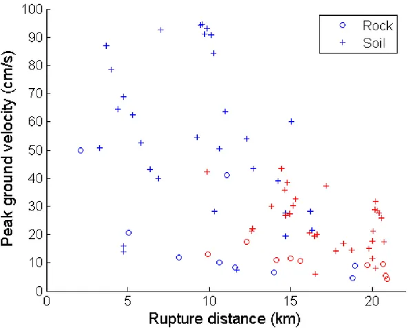
Figure 5. Simulated peak ground velocities for scenario 1 (blue) and scenario 2 (red) against rupture distance.

Figure 5 shows the simulated peak ground velocity (PGV) for the two scenarios against rupture distance. It shows that, as expected, the ground motions decay with distance for rock sites. However, the amplification of ground motions due to the basin and the generation of surface waves mean that PGV values at sites within the basin do not show much decay with distance. It is remarkable that the PGV at station 4 (at about 11km) on rock for scenario 1 is large (42 cm/s). This station is located on the extension of the earthquake fault, so this large value may be attributable to strong directivity and a maximum within the radiation pattern for shear waves.

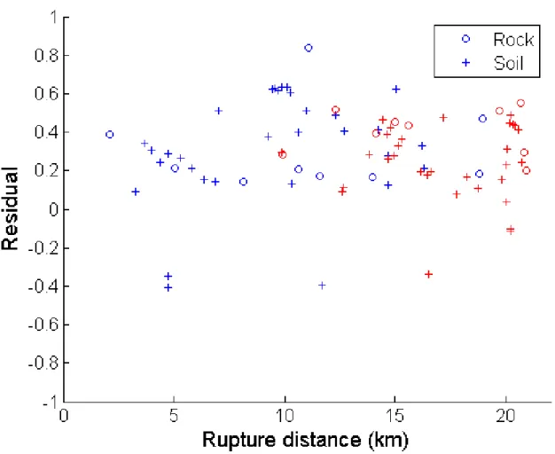
Figure 6 shows the computed residuals for both scenarios using the model of Campbell (1997) with respect to rupture distance. The pattern of residuals is similar for the other empirical models although the absolute value of the residuals changes. Table I lists the mean and standard deviation of the residuals for the five empirical models for both rock and soil stations. The figure and the table show that, in general, the simulated PGV values are reasonably well predicted, however, ground motions in the basin are, in general, underestimated by an average factor of two to three times.

Figure 6. Residuals using model of Campbell (1997) for scenario 1 (blue) and scenario 2 (red) against rupture distance.

Table I. Mean residuals for the five empirical models for rock and soil sites

Model Mean and standard

deviation of residuals (rock)

Mean and standard deviation of residuals (soil)

Campbell (1997) 0.36 (0.18) 0.27 (0.25)

Sadigh & Egan (1998) 0.10 (0.19) 0.40 (0.25)

Chapman (1999) 0.21 (0.19) 0.35 (0.25)

Tromans & Bommer (2002) 0.23 (0.18) 0.43 (0.23)

Pankow & Pechmann (2004) 0.21 (0.19) 0.45 (0.24)

As a continuation of the work present here, it would be interesting to compare the simulated long-period motions within the basin with those predicted by the recent models of basin effects developed for use in California (e.g. Joyner, 2000; Choi et al., 2005). These models use the depth to the bedrock and, for some models, the distance from the edge of the basin to the site.

4. Conclusions

Numerical simulations of wave propagation in the Grenoble basin are carried out using a FDM for a few earthquake scenarios. The obtained ground motions are compared with the observed ground motions at the given stations, within the simulations for different

numerical procedures and with empirical equations. The equations derived by Campbell (1997) better match the simulations for the rock sites outside the basin than for the soil sites within the basin. It is remarkable that PGVs at some basin sites show changes of several times at the same distance from the earthquake fault. We also observe strong directivity effects from rupture propagation along the fault. The obtained scatter is compatible with other simulations which we have performed recently (Aochi and Douglas, 2006; Douglas et al., 2006) so that this is considered to be inherent due to the complexity in the rupture process and the crust structure models.

5. Acknowledgements

We first appreciate the effort of the organizers at LGIT Grenoble for preparing this benchmark test. The basic simulations of this study have been carried out as a part of the European project Interreg SISMOVALP (Seismic Movements of Alpine Valleys, 2003-2006) and the French national project SISMODT (2004-2003-2006) funded by MEDD. A part of the comparison between the simulated ground motions with empirical equations is a contribution to the national project QSHA (Quantitative Seismic Hazard Analysis, 2006-2008) funded by ANR. The high performance simulations with fine grids were undertaken by the Computational System and Technology division (STI) of BRGM in the framework of the national project NUMASIS (2006-2008) funded by ANR. This work is also a general contribution to the seismic risk research project of BRGM (SEISMORISK).

6. References

Ambraseys, N. N., M. W. Free (1997) Surface-wave magnitude calibration for European region earthquakes, Journal of Earthquake Engineering, 1(1), 1–22.

Aochi, H., J. Douglas. Testing the validity of simulated strong ground motion from the dynamic rupture of a finite fault, by using empirical equations. Bulletin of Earthquake Engineering. In press.

Aochi, H., R. Madariaga (2003), The 1999 Izmit, Turkey, earthquake: Nonplanar fault structure, dynamic rupture process, and strong ground motion. Bulletin of the Seismological Society of America, 93(3), 1249–1266.

Campbell, K. W. (1997), Empirical near-source attenuation relationships for horizontal and vertical components of peak ground acceleration, peak ground velocity, and pseudo-absolute acceleration response spectra,” Seismological Research Letters, 68(1), 154–179.

Chapman, M.C. (1999), On the use of elastic input energy for seismic hazard analysis, Earthquake Spectra, 15(4), 607-635.

Choi, Y., J. P. Stewart, R. W. Graves (2005), Empirical model for basin effects accounts for basin depth and source location, Bulletin of the Seismological Society of America, 95(4), 1412-1427.

Collino, F., Tsogka, C. (2001) Application of the Perfectly Matched Absorbing Layer Model to the Linear Elastodynamic Problem in Anisotropic Heterogeneous Media, Geophysics, 66, 294–307.

Douglas, J., H. Aochi, P. Suhadolc, G. Costa (2006), The importance of crustal structure in explaining the observed uncertainties in ground motion estimation. Bulletin of Earthquake Engineering, submitted. Graves, R. W. J. (1996), Simulating seismic wave propagation in 3D elastic media using staggered grid

finite differences. Bulletin of the Seismological Society of America, 86(4),1091–1106.

Joyner, W. B. (2000), Strong motion from surface waves in deep sedimentary basins, Bulletin of the Seismological Society of America, 90 (6B), S95-S112.

Levander, A. R. (1988), Fourth-order finite-difference P-SV seismograms. Geophysics, 53, 1425-1436. Olsen, K. B. (1994), Simulation of three-dimensional wave propagation in the Salt Lake Basin. Ph.D. thesis,

University of Utah.

Olsen, K. B., E. Fukuyama, H. Aochi, R. Madaraiaga (1999) Hybrid Modeling of Curved Fault Radiation in a 3D Heterogeneous Medium, 2nd ACES Workshop Proceedings (ed. M. Matsu’ura, K. Nakajima and P. Mora) pp 343–349.

Pankow, K. L., J. C. Pechmann, J. C. (2004) The SEA99 ground-motion predictive relations and new peak ground velocity relation, Bulletin of the Seismological Society of America, 94(1), 341–348.

Sadigh, R. K., J. A. Egan, (1998), Updated relationships for horizontal peak ground velocity and peak ground displacements for shallow crustal earthquakes, Proceedings of the Sixth US National Conference on Earthquake Engineering, Seattle, Paper No. 317.

Tromans, I. J., J. J. Bommer (2002), The attenuation of strong-motion peaks in Europe, Proceedings of the Twelfth European Conference on Earthquake Engineering, London, Paper 394.