Modeling of plasma transport and negative ion extraction in a magnetized radio-frequency plasma source

(1)

HAL Id: hal-02326878

https://hal.archives-ouvertes.fr/hal-02326878

Submitted on 22 Oct 2019

HAL is a multi-disciplinary open access

archive for the deposit and dissemination of

sci-entific research documents, whether they are

pub-lished or not. The documents may come from

teaching and research institutions in France or

abroad, or from public or private research centers.

L’archive ouverte pluridisciplinaire HAL, est

destinée au dépôt et à la diffusion de documents

scientifiques de niveau recherche, publiés ou non,

émanant des établissements d’enseignement et de

recherche français ou étrangers, des laboratoires

publics ou privés.

extraction in a magnetized radio-frequency plasma

source

Gwenaël Fubiani, Laurent Garrigues, G J M Hagelaar, Nicolas Kohen,

Jean-Pierre Boeuf

To cite this version:

Gwenaël Fubiani, Laurent Garrigues, G J M Hagelaar, Nicolas Kohen, Jean-Pierre Boeuf. Modeling

of plasma transport and negative ion extraction in a magnetized radio-frequency plasma source. New

Journal of Physics, Institute of Physics: Open Access Journals, 2017, 19 (1), pp.015002.

�10.1088/1367-2630/19/1/015002�. �hal-02326878�

(2)

This content has been downloaded from IOPscience. Please scroll down to see the full text.

Download details:

IP Address: 130.120.99.16

This content was downloaded on 11/01/2017 at 11:41 Please note that terms and conditions apply.

Modeling of plasma transport and negative ion extraction in a magnetized radio-frequency

plasma source

View the table of contents for this issue, or go to the journal homepage for more 2017 New J. Phys. 19 015002

(http://iopscience.iop.org/1367-2630/19/1/015002)

Modeling of plasma transport and negative ion extraction in a

magnetized radio-frequency plasma source

G Fubiani, L Garrigues, G Hagelaar, N Kohen and J P Boeuf LAPLACE, Université de Toulouse, CNRS, INPT, UPS, France

E-mail:gwenael.fubiani@laplace.univ-tlse.fr

Keywords: modeling, negative ions, particle in cell, plasma, ITER, ion source

Abstract

Negative ion sources for fusion are high densities plasma sources in large discharge volumes. There are

many challenges in the modeling of these sources, due to numerical constraints associated with the

high plasma density, to the coupling between plasma and neutral transport and chemistry, the

presence of a magnetic

ﬁlter, and the extraction of negative ions. In this paper we present recent results

concerning these different aspects. Emphasis is put on the modeling approach and on the methods

and approximations. The models are not fully predictive and not complete as would be engineering

codes but they are used to identify the basic principles and to better understand the physics of the

negative ion sources.

1. Introduction

Negative ion sources are used in a variety of researchﬁelds and applications [1] such as in tandem type

electrostatic accelerators, cyclotrons, storage rings in synchrotrons, nuclear and particle physics(for instance to produce neutrons in the Spallation Neutron Source[2]) and in magnetic fusion devices (generation of high

power neutral beams[3]). High brightness negative ion sources (i.e., which produces large negative ion currents)

use cesium vapor to signiﬁcantly enhance the production of negative ions on the source cathode surface. Cesium lowers the work function of the metal and hence facilitates the transfer of an electron from the metal surface to a neutral hydrogen atom by a tunneling process. The main types of devices that use cesium are magnetrons, Penning and multi-cusps ion sources. The former have applications in accelerators and the latter are often large volume ion sources like those developed for fusion applications. The plasma in large volume devices can be generated by hot cathodes(heated ﬁlaments) or radio-frequency (RF) antennas (inductively coupled-plasma, ICP discharges) standing either inside or outside the discharge [1]. Ion sources for fusion are tandem type

devices with a so-called expansion chamber juxtaposed next to the discharge region. The expansion chamber is often magnetized with magneticfield lines perpendicular to the electron flux exiting the discharge. The magnetic field strength is typically of the order of ∼100 G and is generated either by permanent magnets placed along the lateral walls of the ion source or via a large currentflowing through the plasma electrode (which is also called ‘plasma grid’). The plasma grid (PG) separates the ion source plasma from the accelerator region, where the extracted negative ions are accelerated to high energies. The axial electron mobility is strongly reduced by the magneticfield inside the expansion chamber and the electron temperature is hence significantly reduced as electrons loose a large amount of energy through collisions. In ion sources for fusion, the background gas pressure(either hydrogen or deuterium type) is ∼0.3Pa and the electron temperature is of the order of 10eV in the discharge region. The magneticfilter reduces the electron temperature down to the eV level in the extraction region, close to the PG. The role of the magneticfilter field in the expansion chamber is threefold: (i) a large versus low electron temperature between the discharge and the extraction region allows the production of negative ions through the dissociative impact between an electron and an hydrogen(or deuterium) molecule

n

(  )

H2 4, whereν is the vibrational level. The vibrational excitation of the hydrogen molecule is maximized at high electron temperatures(typicallyTe~10eV) while the cross-section for the dissociative attachment ofH2

and hence the production of a negative ion is the largest forTe~1 eV.(ii) A low electron temperature in the

OPEN ACCESS

RECEIVED

8 September 2016

REVISED

24 November 2016

ACCEPTED FOR PUBLICATION

29 November 2016

PUBLISHED

6 January 2017 Original content from this work may be used under the terms of theCreative Commons Attribution 3.0 licence.

Any further distribution of this work must maintain attribution to the author(s) and the title of the work, journal citation and DOI.

(4)

vicinity of the PG significantly increases the survival rate of the negative ions and (iii) the magnetic filter more or less lowers the electronflux onto the PG but this is not sufficient and a suppression magnetic field is used to limit the co-extracted electron current. Co-extracted electrons have a damaging effect inside the electrostatic

accelerator[4]. The electron beam is unfocused and induces a large parasitic power deposition on the accelerator

parts. Note that in fusion-type, high power, large volume and low pressure ion sources, negatives ions produced via dissociative attachment of the background gas molecules(so called ‘volume processes’) range between 10%– 20% of the total amount of extracted negative ion current[5,6], the remaining part corresponds to ions

generated on the cesiated PG surface through neutral atom and positive ion impacts. In magnetic fusion applications, negative ion sources are a subset of a neutral beam injector(NBI) producing high power neutral beams which are injected into the Tokamak plasma. Neutrals are insensitive to magneticfields and can hence penetrate into the hot plasma core. The neutral beam provides power to the plasma, current(which is necessary to sustain the poloidalfield) and are helpful to minimize the buildup of some type of instabilities. In the future International Thermonuclear Experimental Reactor(ITER), NBIs are designed to inject 33MW of power (split over two beam lines) with an energy of 1MeV into the Tokamak plasma [7]. The ITER project is the first fusion

device which will mainly be heated by alpha particles(H_e2+). The plasma will consist of Deuterium and Tritium ions providing 500MW of fusion power. 50MW of additional external power will be necessary in order to heat and control the plasma during the operating phase while the alpha particles will re-inject 100MW of power to the fusion plasma(the total heating power is 150 MW). The remaining 400 MW is carried by the neutrons toward the wall of the Tokamak[8]. The external heating system for ITER also includes 20MW of electron

cyclotron heating at 170GHz and 20MW of ion cyclotron heating in the –35 65 MHz frequency range[9]. Total

power is consequently 73MW (including neutral beams), slightly above the required 50MW for ITER. In this paper we illustrate and analyze, on the basis of new results, the work performed in our group in the last ten years on the modeling and simulation of the negative ion source and negative ion extraction. The modeling of the negative ion source in all its complexity(power absorption, plasma chemistry, coupling with neutral transport and chemistry, transport across magneticﬁeld, negative ion production and extraction) is a formidable task and we address the different questions separately with dedicated models using simplifying assumptions. In most cases the models are applied to the ITER prototype negative ion source BATMAN[5,10– 12] (BAvarian Test MAchine for Negative ions) developed at the Max-Planck-Institut für Plasmaphysik,

Garching, Germany. The source is a tandem type device similar to the ITER conﬁguration but with one ICP discharge(driver) and a smaller expansion chamber volume, accordingly. The driver dimensions are a cylinder of diameter 24.5cm and length 16cm [11,13]. An external cylindrical antenna confers to the background gas

(either molecular hydrogen or deuterium) about 100kW of RF power, which generates a high density plasma of the order of4´10 m17 -3_{(averaged over the whole ion source volume). The expansion chamber, which is}

connected to the driver, has a larger volume and is magnetized; its size is approximately 57.9cm in height, width of 30.9 and 24.4cm in depth.

Most results presented and discussed in this paper have been obtained with particle-in-cell Monte Carlo collisions(PIC-MCC) methods. In section2we describe in details the method and discuss different points such as(1) parallelization, (2) use of scaling to make the simulations more tractable, (3) 3D versus 2D and 2.5D calculations,(4) a method for injecting power into the plasma (electron heating), (5) implementation of collisions(including physical-chemistry) and lastly (6) the modeling of the production of negative ions on the PG surface.

The negative ion source is a high density plasma in a large volume, i.e. the Debye length is much smaller than the dimensions of the source. The strong constraints on the grid spacing and time steps of a PIC-MCC

simulation make it difficult to deal with the real values of the plasma density or dimensions. In several recent publications we have been using scaling of the plasma density(or, equivalently, of the vacuum permittivity) to keep the computation time within reasonable limits. Section3is devoted to the study of the effect of density scaling on the simulation results in a simplified problem of plasma transport across a magnetic filter where the Hall effect contributes to the cross-field transport and leads to plasma asymmetry (as in the ITER negative ion source).

We have previously published the results of aﬂuid model of the negative ion source where the plasma properties were analyzed as a function of power and pressure[14,15]. The plasma ﬂuid model was coupled to a

ﬂuid description of the neutral transport and chemistry. Interesting outcomes of the simulation were the strong neutral depletion due to gas heating and ionization, and the high temperature of hydrogen atoms with respect to molecules. The Knudsen number can be close to one in the negative ion source and this may have consequences on the velocity distribution functions of neutral particles. In section4we look at the possible effects of the low gas density on neutral transport and on the velocity distribution of hydrogen atoms and molecules. The particle transport in this section is described by a direct-simulation-Monte-Carlo(DSMC) model.

In section5, we provide a detailed description of the plasma transport across the magneticfilter field inside the expansion chamber of the ion source(potential profiles, electron density and temperature). We discuss the

(5)

incidence of the Hall effect on the plasma dynamics(induction of a transverse asymmetry), the kinetics of negative ions and the role of positive ions in the production of negative ions on the cesiated surface of the PG. Section6compares the model predictions with experimental measurements. We show that the plasma asymmetry(and hence the incidence of the Hall effect) is observed in both cases. Section7analyses the numerical issues associated with the modeling of negative ion extraction from the PG surface. The simulation geometry is restricted to a zoom around a single aperture. PIC simulations are difﬁcult to use with the real values of the plasma density. We present calculations obtained for plasma densities lower than in a real negative ion source and discuss the possible scaling laws that can be use to extrapolate the results to more realistic conditions.

2. Numerical model

2.1. PIC simulations

The principles of the PIC-MCCs method are described in textbooks[16,17] and in various publications. In this

section we discuss some specific issues associated with the simulation of ITER-type negative ion sources, i.e. (1) need to use parallel computing,(2) difficulty to simulate the high plasma density conditions of these sources (and consequences of performing density scaling), (3) 2D versus 2.5D and 3D calculations (4) implementation of a simplified model for the external power absorption inside the ICP discharge, (5) hydrogen plasma chemistry and(6) on the method to model the generation of negative ions onto the cesiated PG surface.

2.1.1. General features and parallelization of PIC-MCC simulation

We have developed and used 2D and 3D parallel Cartesian electrostatic explicit PIC-MCC models[16,17] to

study the plasma of negative ion sources for fusion. Due to he strong constraints on the grid spacing and time step in the high density plasma of negative ion sources, the PIC method must be optimized and parallelized. In this section we recall the principles of PIC-MCC simulations and brieﬂy describe the technique of parallelization that is used in our models and its performance in term of computer time as a function of number of computer cores(or threads).

In an explicit algorithm, the particle trajectories are calculated based on thefields evaluated at the previous time step. The(self) electric field is derived self-consistently from the densities estimated on the grid nodes of the simulation domain. The magneticfields, filter and suppression fields (the latter is generated by permanent magnets embedded in thefirst grid of the accelerator), are prescribed in this work. The time step must be a fraction of the electron plasma period and the grid size close to the electron Debye length, accordingly(both are set by the lightest of the simulated particles). The parallelization is performed in an hybrid manner using OpenMP[18] and MPI libraries. We use a particle-decomposition scheme for the particle pusher where each

core(thread) have access to the whole simulation domain (as opposed to a domain-decomposition approach). The number of particles per core is nearly identical. We further implemented a sorting algorithm[19] in order to

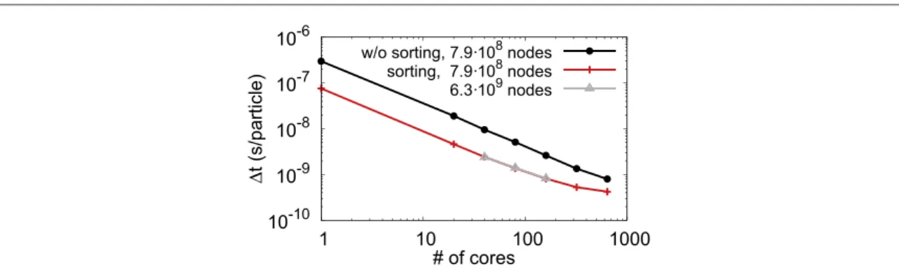
limit the access to the computer memory(RAM) and boost the execution time, Dtpush, of the pusher subroutine.

The latter includes electron heating(inside the ICP discharge), field interpolations, update of the velocities and positions together with the charge deposition on the grid nodes. Particles are sorted per grid cell. Thefield and density arrays are hence accessed sequentially. Dtpushis shown infigure1normalized to the number of particles

in the simulation. The best performance is obtained by attaching a MPI thread per socket and a number of OpenMP thread identical to the number of cores per socket. For the simulations offigure1, we set the number of OpenMP threads to 10. We sort particles every 10 time steps without any loss of performance. The calculation is performed with a 3D PIC-MCC model and the numerical resolution is either96 ´64´128 grid nodes or eight times larger with 80 particles-per-cell(ppc). The time gained in the pusher with the particle sorting is a factor∼4. The sorting algorithm remains efficient as long as there is on average at least one particle per cell per thread. Beyond this limit Dtpushconverges toward the value without sorting as shown infigure1. We define the

efﬁciency of the pusher without sorting as,

b = D D ( ) ( ) t t N , 1 push 1 push core

whereNcoreis the number of cores(threads) and Dtpush( )1 the execution time of the pusher forNcore=1.β should

be equal to 1 for a perfect parallelization of the pusher. Weﬁnd b78% for 20 cores, 70% for 320 cores and lastly, dropping to∼60% for 640 cores (i.e., about 23% loss in efﬁciency with respect to 20 cores).

Poisson’s equation is solved iteratively on the grid nodes with a 3D multi-grid solver [20]. The latter is

parallelized via a domain-decomposition approach. In multi-grid algorithms, a hierarchy of discretizations(i.e., grids) is implemented. A relaxation method (so-called successive-over-relaxation, SOR, in our case) is applied successively on the different grid levels(from ﬁne to coarse grid levels and vice versa). Multigrid algorithms hence accelerate the convergence of a basic iterative method because of the fast reduction of short-wavelength

(6)

errors by cycling through the different sub-grid levels. Each sub-domain(i.e., a slice of the simulated geometry) is attached to a MPI thread while the do-loops are parallelized with OpenMP(SOR, restriction and prolongation subroutines[20]). Once there is less that one node per MPI thread in the direction where the physical domain is

decomposed then the numerical grid is merged between all the MPI thread. The parallelization for the coarsest grids in consequently only achieved by the OpenMP threads. This is clearly a limiting factor and more work is needed to further improve the algorithm. As an example, using a mesh of 5123nodes, the speedup is about∼30 for 80 cores(b 40%). The execution time of the Poisson solver (normalized to the number of grid nodes) versus the number of cores in the simulation is shown inﬁgure2.

Lastly, for the numerical resolution which we typically implement to characterize the plasma properties of the ITER-prototype ion source at BATMAN, that is,192 ´128´256 grid nodes with 20 ppc, the fraction of the execution time per subroutine averaged over one time step is,∼55% for the particle pusher, ∼8% for the Poisson solver,∼16% for Monte-Carlo (MC) collisions, ∼4% for the sorting. The remaining time concerns both the evaluation of the electricﬁeld and the calculation of the total charge density on the grid nodes (which involve some communication between MPI threads).

2.1.2. Scaling of PIC-MCC simulations

The high plasma density and large volume of negative ion sources make it practically impossible to perform multi-dimensional PIC-MCC simulations for real conditions. The ratio of discharge dimension to Debye length is on the order of 104(tens of centimeters versus tens of micrometers) so a simple 2D PIC-MCC simulation in real conditions would involve 108grid points and more than 109super-particles. This is clearly prohibitive for parametric studies with 2D simulations and impossible for 3D. The 3D simulation of negative ion extraction is also difﬁcult although the plasma density there is smaller than in the driver and one generally consider a small simulation domain around a grid aperture.

To overcome this problem, one solution is to perform some‘scaling’ i.e. to run the simulations for more tractable conditions(e.g. smaller plasma densities or smaller dimensions) and extrapolate the results to the real conditions by using some scaling laws[21–24]. The simplest scaling is the scaling on plasma density. The

Figure 1. Execution time of the particle pusher(per time step) normalized to the number of macroparticles in the simulation versus the number of cores. The time is shown either with(red and gray lines) or without implementing a sorting algorithm (black-line). We use 80 particles-per-cell(ppc), a numerical resolution of96´64´128grid nodes(black and red lines) and192´128´256(gray line). The calculation is performed with a 3D PIC-MCC model on a 10 cores Intel Xeon processor E5-2680 v2 (25M cache, 2.80 GHz). There is 2 sockets per CPU, 20 cores in total.

Figure 2. Execution time of the geometric multigrid Poisson solver(per time step) normalized to the number of grid nodes in the simulation versus the number of cores. the numerical resolution is 5123_{(black line), 1024}3_{(red) and 2048}3_{(gray) grid nodes,}

respectively. The calculation is performed on a 10 cores Intel Xeon processor E5-2680 v2_{(25M cache, 2.80 GHz). We set the number} of OpenMP threads to 10.

(7)

Boltzmann equation for electrons or ions is linear in the density of charged particles if the collision term is linear (i.e. when only charged particle collisions with neutrals are considered, with a given, constant velocity

distribution function of neutral species), i.e. the equation is invariant if the distribution function (hence the charged particle density) f is divided by a constant α:

a a a a ¶ ¶ + ¶ ¶ + ¶ ¶ = - - -[ ] ( ) f t f f I f v r a v . . , 2 1 1 1 1

whereais the acceleration of the charged particles due to the Lorentz force:

= q ( + ´ ) ( )

m

a E v B , 3

and I is the collision operator.

In a quasineutral plasma, the electricﬁeld is deduced from current continuity and is invariant when the plasma density n is divided by a constantα. This can be easily seen on the electron and ion momentum equations (from which the total current density can be deduced). A simpliﬁed form of the electron current density is:

n

- ´ = - +P m ( )

E J B J

ene e e en e, 4

whereJeis the electron current density, Pethe electron pressure andnenthe electron-neutral collision frequency.

In this equation, the electricﬁeld is invariant when the electron density is multiplied by a given factor. A similar argument can be made for ions.

Therefore we can conclude that the properties of a quasineutral plasma are not changed when the plasma density is scaled by a constant factor(for linear collision terms) and a PIC-MCC simulation of a quasineutral plasma can be performed with scaled densities. In a real problem the plasma is bounded which implies the presence of non-neutral Debye sheaths next to the walls. The sheath properties are clearly not invariant with a scaling of the plasma density(the sheath length is generally proportional to the Debye length), but the sheath voltage and hence the plasma potential do not depend on plasma density(the plasma potential depends only of the electron temperature and electron to ion mass ratio). Therefore, when a PIC-MCC simulation is performed with scaled densities(i.e. plasma density smaller that the real density) only the wall sheath thickness is modiﬁed. If the sheath thickness is still much smaller than the discharge dimensions the scaled simulation gives an accurate description of the real problem. However, care must be taken in the following situations:

• Since the sheath is larger for lower plasma densities it may become more collisional. The charged particle ﬂuxes to the walls may be modiﬁed if the scaling is too important (ionization can also take place and be enhanced by secondary emission if present).

• In a magnetized plasma, the ratio of the charged particle gyroradius to the sheath length is also modified by the density scaling. This may also impact the charged particle transport and charged particlefluxes to the walls. • The properties of the ion beam extracted from the plasma source are modified by the plasma density for a

given extraction voltage(Child Langmuir law in the case of a collisionless sheath) and therefore the applied voltage should be scaled accordingly. This is clearly an important issue when scaling is used in a model of negative ion extraction(see section7.5).

• In the presence of instabilities or turbulence associated with space charge separation (e.g. in a magnetized plasma) the density scaling no longer works. The instabilities and associated anomalous transport across the magneticﬁeld do not scale linearly with the plasma density and density scaling cannot be used.

If Coulomb collisions(or other nonlinear collisions such as electron–ion recombination) are important in the real conditions, the collision module of the scaled PIC-MCC simulation can easily be modiﬁed to take into account the real collision frequencies(by using the real value of the target particle densities instead of the scaled value).

Note that in some published papers the scaling used is presented as a scaling of the vacuum permittivity instead of a scaling of the density[21–23]. It is easy to see (in Poisson’s equation) that dividing the plasma density

by a factorα is exactly equivalent to multiplying the vacuum permittivity by the same factor. In that case no scaling needs to be done for Coulomb collisions since the plasma density in the simulation is the real one.

Finally some authors have been using scaling on the discharge dimensions instead of a density scaling(see, eg,[25,26]). In a quasineutral plasma, the system formed by the Boltzmann equations coupled with the

generalized Ohm’s law is invariant when the dimensions are reduced by a factor β provided that the gas density (i.e. collision operator) and magnetic ﬁeld are multiplied by β (the time scale is also divided by β). The

(8)

b b ¶ ¶ + ¶ ¶ + ¶ ¶ = [ ] ( ) f t f f I f v r a v . . . 5

We see that this equation is invariant if the collision term is multiplied byβ, i.e. if the gas density is multiplied byβ (the collision term is proportional to the gas density in the absence of Coulomb collisions), and if the acceleration,a= q(E+ ´v B)

m is multiplied byβ. The electric ﬁeld E being a potential gradient is

automatically multiplied byβ when the dimensions are reduced by the same factor, while the external magnetic ﬁeld B must be multiplied by β.

The scaling, deﬁned above, on density, permittivity and dimensions, are all equivalent since in these three cases, the ratios l Lc and rL Lare the same as in the real problem while the ratio lD Lis larger than in the real

problem by a factor a1 2_{in the density scaling and by a factor}_{β in the dimensions scaling. The density scaling}

and dimensions scaling are therefore strictly identical, for a quasineutral plasma, ifb =a1 2_{. l}

c, rL,lD, and L

are respectively the charged particle mean free paths, Larmor radii, Debye lengths, and discharge dimensions. 2.1.3. 2D, 2.5D, and 3D simulations

3D PIC-MCC calculations are restricted to low plasma densities, typically ~10 m13 -3_{on 40 cores with}

´ ´

192 128 256 grid nodes(20 ppc) for the prototype source at BATMAN. The density is about 105times lower than the real density(i.e. a = 105_{, see previous sub-section). In 2D rectangular PIC simulations, on the}

other hand, one may simulate a significantly larger plasma density. The plasma in the direction perpendicular to the simulation domain is implicitly supposed to be uniform and infinite and no charged particle losses along this direction are taken into account. A solution that allows to implement approximately the charged particle losses in the direction perpendicular to a 2D simulation domain without performing a 3D calculation is the so-called 2.5D model[23,24]. For magnetized plasmas, the particle transport is simulated in the plane perpendicular toB (i.e. where the magnetized drift motion takes place). We assume that the plasma is uniform along the un-simulated direction, perpendicular to the 2D simulation plane(i.e., parallel to the magnetic field lines), and we use the following considerations to estimates the charged particle losses:

• The ion dynamics in the direction perpendicular to the 2D simulation plane is not calculated but we estimate the ion losses from the Bohmﬂuxes to the walls. The loss frequency at a given location in the simulation plane is obtained from[27] n = hu LL 2 B y, whereuB= eT x ze( , ) miis the local Bohm velocity, Lyis the length of

the ion source in the third dimension,h=ns á ñn 0.5, nsis the local plasma density at the sheath edge, á ñn

the averaged density, Te(mi), the local electron temperature (ion mass), respectively.

• The electron and negative ion trajectories are followed in the third dimension assuming that the plasma potential isﬂat (i.e., no electric ﬁeld). When a negatively charged particle reaches a wall, it is removed if its kinetic energy along the un-simulated dimension is greater than the difference between the plasma potential and the wall, i.e.,1 2m v_{i z}2f (x z, )for a grounded wall. miis the particle mass.

Macroparticles are created anywhere between0 y Lyin the third dimension(via ionization processes).

The 2.5D model estimates plasma characteristics which are averaged over Ly. Note that this model is restricted to

simplified magnetic field maps, where the field lines are straight in the un-simulated direction. The comparison between 2D, 2.5D and 3D models has been extensively discussed in[23].

2.1.4. External RF power absorption and Maxwellian heating in the driver

The ITER-type tandem reactors have an ICP discharge which couples a high RF power(typically 100 kW at 1 MHz frequency) to a hydrogen or deuterium plasma. We do not simulate directly the interaction of the RF ﬁeld with the plasma but assume instead, a given absorbed power. Every time step, macroparticles which are found inside the region of RF power deposition are heated according to some artiﬁcial heating collision frequency. Electrons, being the lightest particles, are assumed to absorb all of the external power. Redistribution of energy to the heavier ions and neutrals is done through collisions(both elastic and inelastic) and the ambipolar potential. Electrons undergoing a heating collision have their velocities replaced by a new set sampled from a Maxwellian distribution with a temperature calculated from the average specie energy(inside the power deposition region) added to the absorbed energy per colliding particles, i.e.,

n = á ñ + ( ) T E P eN 3 2 h kh , 6 abs eh h

where Th(eV) is the heating temperature in electron-Volts (eV), á ñEk his the average electron energy,Pabs(W) is

the absorbed power, nhthe heating frequency and Nehthe number of electrons, respectively. For a given time

step,Nemn Dh tcolliding macro-electrons are chosen randomly where Nemis the total number of macroparticles

(9)

The simulated electron temperature proﬁle is constant inside the discharge region. This is consistent with plasma conditions which are found in devices running at low pressure, low RF frequency(∼1 MHz) where electrons have typically a large thermal velocity in the driver(Te~10eV), and a low collision frequency (a mean-free-path of the order of the discharge radius). These non-local heating conditions allow electrons, which can move freely, to deposit energy over the whole driver volume. Kinetic effects such as collisionless heating (leading to a so-called anomalous skin depth) and a non-negligible ponderomotive force (due to the high power and the low frequency of the RF antenna) are also expected inside the ICP discharge. The electron distribution function is typically non-Maxwellian in these conditions. A complete self-consistent model of the energy coupling in the ICP would be required to obtain a better estimation of the electron distribution in the driver. A non-self-consistent but much simpler and useful approach would be to study the inﬂuence of a non-Maxwellian distribution on the plasma parameters by imposing in the driver electron distributions that are deduced from experiments.

2.1.5. Implementation of collisions in a particle model—MC and DSMC methods In a PIC-MCC algorithm, the Boltzmann equation,

¶ ¶ + ¶ ¶ + ¶ ¶ = ¶ ¶ ( ) ⎛ ⎝ ⎜ ⎞ ⎠ ⎟ f t f f f t v r a v . . , 7 i i i i c

is solved numerically in two steps[28,29].

å

s ¶ ¶ =

∬

( ¢ ¢ - ) W ( ) ⎛ ⎝ ⎜ f ⎞_⎠⎟ t f f f f v d d ,v 8 i c t i t i t r tT t

is the collision operator, fi( ft) is the distribution function for the incident (target) specie, respectively, mithe

mass, F the forceﬁeld, =vr ∣vi-vt∣the relative velocity, s ( )tT vr the total differential cross-section(summed

over all the collision processes between the incident and the target particles) and, lastly, Ω the solid angle. Primes denote the distribution function after the collision. For small time steps, equation(7) may be rewritten as,

+ D = + D + D

( ) ( )( ) ( ) ( )

f x v t_i , , t 1 tI 1 tD f x v t_i , , , 9 wheref x v t_i( , , )is known explicitly from the previous time step. Thisﬁnite-difference analog of equation (7) is

second order correct inDt. The operators D and I are,

= - ¶ ¶ -¶ ¶ ( ) ( ) D f v f f r a v . . , 10 i i i

andI f( )_i = ¶ ¶( f_i t)c. Applying the operator( - DtD1 ) on the distribution function fiis equivalent to solving

the Vlasov equation,

¶ ¶ + ¶ ¶ + ¶ ¶ = ( ) f t f f v r a v . . 0. 11 i i i

The PIC procedure[16,17] is a characteristic solution of equation (11). Once the particle trajectories have been

updated, then the second operator( - DtI1 ) may be applied on the (updated) distribution function. A macroparticle is equivalent to a Dirac delta function in position-velocity space(Eulerian representation of a point particle) and hence a probability may be derived from equation (9) for each collision processes [28,29].

The probability for an incident particle to undergo an elastic or inelastic collision with a target particle during a time stepDtis

å

s = D = ( )Pi t (n v) , (12) c N c c r max 1 max c

with Nccorresponding to the total number of reactions for the incident specie, ncthe density of the target specie

associated with a given collision index andvr=∣vi-vc∣. s( c r maxv) is artiﬁcially set to its maximum value and

hence ( )Pi maxis greater than the real probability and is constant over the entire simulation domain. There is

consequently a probability,

å

= -= ( ) ( ) ( ) P P P 1 , 13 i c N c i null 1 max c

that a particle undergoes a fake collision(dubbed ‘null’ collision), which will be discarded.Pc=nc c r rs( )v vDt.

The total number of incident particles which will hence collide during a time stepDt(including a ‘null’ collision) is,

= ( ) ( )

Nmax N Pi imax, 14

where Niis the number of incident macroparticles in the simulation. Nimust be replaced by(Ni-1 2) for

(10)

particles and consequently the latter may be chosen randomly inside the simulation domain. In the model, one checksﬁrst if the incident macroparticle experienced a real collision,

- ( ) ( )



r 1 Pi null, 15

where r is a random number between 0 and 1. The probabilities Pcfor each reactions(whose total number is Nc

for a given incident specie) are ordered from the smallest to the largest and a reaction k occurred if,

å

= ( ) ( )  r P P . 16 c k c i 1 max

Once a collision type is selected then the macroparticles(both incident and target) are scattered away in the center-of-mass(CM) frame (see next section). In the model, neutrals are either considered as a non-moving background specie with a given density proﬁle or are actually implemented as macroparticles and their

trajectories integrated. In the case of the former, collisions between charged particles and neutrals are performed by the so-called MC method while for the latter, actual particle–particle collisions are evaluated using a DSMC algorithm[30]. Both are similar except that in the MC method, one artiﬁcially extract a neutral particle velocity

from a Maxwellian distribution function. Collisions between charged particles are always performed by a DSMC algorithm in the model. Collisions(both elastic and inelastic), are implemented assuming that particles

(incident, target or newly created) are scattered isotropically in the CM. Energy and momentum is conserved and we assume for simplicity that each byproduct partner after the collision have identical momentum in the CM frame. This implies that the lightest particles will equally share most of the available energy. For further details, please refer to[21].

2.1.6. Physical chemistry of charged particles

We describe below the most complete version of the plasma chemistry module embedded in our PIC-MCC model(we often use a simpliﬁed sub-set of this module, depending on the purpose of the model). In this model, the plasma consists of electrons, molecular hydrogen(background) gasH2, hydrogen atomsH, molecular ions

+

H2 andH+3, protons and lastly negative ionsH-. Collisions between electrons, ions and neutrals are considered;

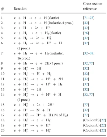
the set of reactions is presented in tables1and2(66 collision processes in total) and is very similar to the one used

by previous authors[15,31]. Table1corresponds to the collision processes associated with electrons. Reactions #2, 6, 7, 8 and 14 combine multiple inelastic processes included in the model in order to correctly account for the electron energy loss. Reaction#2 regroups the excitation of the hydrogen atom from the ground state to the electronic leveln= –2 5[32]. Reaction #7 combines the ground state excitation of the hydrogen molecule

n

S+ =

( )

H X2 1 g; 0 to the vibrational levels n¢ = –1 3[32,33], electronic levels (for alln¢) SB1 u, ¢ SB1 u,  SB1 u,

Table 1. Electron collisions.

# Reaction Cross section reference 1 e + H  e + H(elastic) [71–75] 2 e + H  e + H(inelastic, 4 proc.) [32] 3 e + H  2e + H+ [32] 4 e + H2  e + H2(elastic) [76] 5 e + H2  2e + H+2 [32] 6 _e + _H  _2e + _H+ + _H 2 (2 proc.) [ 32_] 7 e + H2  e + H2(inelastic, 16 proc.) [32–38] 8 e + H2  e + 2H(3 proc.) [32,77] 9 e + H+3  3H [32] 10 e + H+3  H + H2 [32] 11 e + H+3  e + H+ + 2H [32] 12 e + H3+  e + H+ + H2 [32] 13 e + H+2  2H [32] 14 e + H+2  e + H+ + H (2 proc.) [32,77] 15 e + H+2  2e + 2H+ [77] 16 e + H-  2e + H [32] 17 e + H*2  H- + H(1% ofH2) [77] 18 e + H+2  e + H+2 (Coulomb) [22] 19 e + H+  e + H+ (Coulomb) [22] 20 e + H+3  e + H+3 (Coulomb) [22]

(11)

P

C1 u,D1Pu,D¢ P1 u, Sa3 +g,c3Pu,d3Pu[32], Rydberg states [34] and lastly rotational levels J=2 [35,36] and 3

[37,38]. Reaction #17 models in a simple manner the generation of negative ions in the ion source volume,

which are a byproduct of the dissociative impact between an electron and molecular hydrogenH2(n4)[32]. The concentration of excited species is not calculated self-consistently in the model. To estimate the volume production of negative ions, we assume that 1% ofH2molecules are excited in vibrational levels withn  4.

This is in accordance with theH2vibrational distribution function calculated either with a 0D model[39] or a 3D

particle tracking code[40]. Table2summarizes the collision processes of heavy ions with neutrals. Reaction#9 corresponds to the excitation of the hydrogen molecule from the ground state to vibrationally excited levels

n¢ = –1 2[41,42] and to the rotational levels = –J 2 3[43]. To our knowledge there is no reliable data available

for the elastic collision betweenH+₃ and neutral atoms(reaction #2), we consequently use the same cross-section as in reaction#1.

2.1.7. Physical chemistry of neutrals

Cross-sections for collisions between neutrals inside the ion source volume, which are summarized in table2

(reactions #18-20), as well as backscattering, dissociation or recombination probabilities against the ion source walls are required for the modeling of the neutral particle dynamics(and the associated neutral depletion). Table3shows the surface processes and corresponding coefﬁcients. In a low-pressure plasma device such as the one used for fusion applications(ITER or DEMO for instance. DEMO is a concept for the next generation of Tokamaks), the plasma-wall processes have a strong impact on the source characteristics. Low-temperature backscattered molecular hydrogen is assumed to be in thermal equilibrium with the wall. An average

Table 2. Heavy particle processes.

# Reaction Cross section reference 1 H+3 + H2  H3+ + H2(elastic) [78] 2 H+3 + H  H+3 + H(elastic) 3 H+2 + H2  H3+ + H [43,78] 4 H+2 + H2  H2 + H+2 [78] 5 H+2 + H  H+2 + H(elastic) [79] 6 H+ + H  H + H+ [80] 7 H+ + H  H+ + H(elastic) [80] 8 H+ + H2  H+ + H2(elastic) [78] 9 H+ + H2  H+ + H2(inelastic, 4 proc.₎ [41–43,78] 10 H- + H  e + 2H [32] 11 H- + H  e + H2 [32] 12 H- + H2  H- + H2(elastic) [43] 13 _H- + _H  _H- + _H_(elastic) _[₄₃_] 14 H+ + H-  2H(2 proc.) [32] 15 H+ + H-  H+2 + e [32] 16 H- + H2  H2 + H + e [32] 17 _H- + _H  _H + _H- _[₈₁_] 18 H + H  H + H [80] 19 H + H2  H + H2 [80] 20 H2 + H2  H2 + H2 [82]

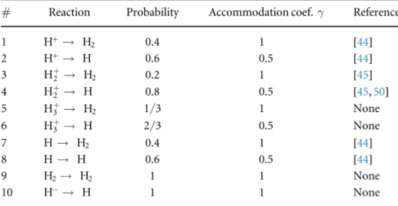
Table 3. Surface processes.

# Reaction Probability Accommodation coef._γ Reference

1 H+ H2 0.4 1 [44] 2 _H+ _H _0.6 _0.5 _[₄₄_] 3 H+2  H2 0.2 1 [45] 4 H+₂  H 0.8 0.5 [45,50] 5 _H+ _H 3 2 1/3 1 None 6 _H+ _H 3 2/3 0.5 None 7 H H2 0.4 1 [44] 8 H H 0.6 0.5 [44] 9 H2 H2 1 1 None 10 H- H 1 1 None

(12)

backscattered energy is considered for fast atoms and ions, i.e. a thermal accommodation coefﬁcientg < 1 (g = 1corresponds to the wall temperature). These estimates are based on Monte Carlo calculations from the code TRIM[44]. Average reﬂection probability is also taken from the same database. Furthermore, we assume

that atoms which are not backscattered will recombine. The interaction ofH+₃andH+₂ions with the walls and the corresponding coefficients are not well known. The coefficients used in the simulations are reported in table3. ForH+₂we use coefficients that are consistent with the measurements of [45]. ForH+₃ we assume guessed values(theH+3 flux to the walls is relatively small with respect to theH+2andH+, and the results are not very

sensitive to these coefﬁcients). 2.1.8. Negative ions

Negative ions are produced on the cesiated PG surface as a byproduct of the impact of hydrogen atoms and positive ions. Our PIC-MCC model has not been coupled to a neutral transport module so the negative ionﬂux emitted by the surface is not obtained self-consistently from aﬂux of neutral atoms deduced from the

simulation. The magnitude of the negative ion current density due to the impact of H atoms on the cesiated PG is either derived from plasma parameters measured experimentally or from DSMC calculations. Assuming a Maxwellian velocity distribution of the hydrogen atoms, theﬂux of these atoms on the PG is:

p G = n eT ( ) m 1 4 8 , 17 H H H H

where nHis the atomic hydrogen density, mHthe mass and e the electronic charge. The negative ion current is

deduced from,

= G

- ( ) ( )

j_H eY TH H, 18

withY T( H)the yield[46], which was not obtained in a plasma (the experiment produced hydrogen from thermal dissociation in a tungsten oven) and consequently remains approximate for the ITER-type ion sources. For typical BATMAN working conditions, weﬁndnH10 m19 -3,TH~1 eVwhich givesjH-~600 A m-2[47– 49]. Negative ions are generated on the PG assuming a Maxwellian ﬂux distribution function with a temperature

=

Tn 1eVin the model. Furthermore, the surface production of negative ions resulting from positive ion impacts is calculated self consistently. For each ion impinging the PG, the yield is evaluated assuming a molecular ion may be considered as an ensemble of protons sharing the incident ion kinetic energy(aH+₃ion for instance would be equivalent to three protons each with an energyE Hk( +)=E Hk( 3+) 3). Each of these ‘protons’ may produce a negative ion. The condition r Ymust be fulﬁlled for the negative ion to be generated with r a

random number between 0 and 1. The yield is taken from Seidl et al[46] for Mo/Cs surface with dynamic

cesiation. The negative ions are scattered isotropically toward the ion source volume with a kinetic energy assumed to beE Hk( -)=E Hk( +) 2. There is experimental evidence that negative ions may capture a large amount of the incident positive ion energy[50]. In addition, for clean metallic surfaces (tungsten) the reﬂected

atomic hydrogen particle energy is numerically evaluated to be around 65% of the impact energy at normal incidence and forEk=1 eV[51]. Lastly, it has been reported in the experiments that the extracted negative ion current increases only slightly with cesium when the PG is water-cooled[52] while a PG heated to a temperature

of ~100 C –250◦C induces a signiﬁcant increase of the negative ion current, by a factor ~ –4 5 in the experimental conditions of[5,52] (the other walls of the ion-source were water-cooled). In the model, we consequently

assume that negative ions may only be produced on the cesiated PG surface. 2.2. Simulation domain

The simulation domain for the 3D PIC-MCC modeling of the BATMAN device is shown inﬁgures3(a) and (b).

The magneticfilter field is generated in the model by permanent magnet bars which are located on the lateral side of the ion source walls close to the PG. Thefield is calculated by a third-party code [53]. In 2.5D, solely the

XZ plane is considered(ﬁgure3(b)) but with a higher numerical resolution (or similarly plasma density) than in

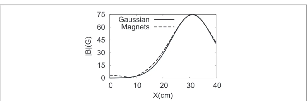
3D. We assumedLy=32 cmfor both the driver and the expansion chamber and we implemented a Gaussian proﬁle for the magnetic ﬁlter (i.e., mirror effects are neglected [23]),

= -( ) ⎡ ( ) ( ) ⎣ ⎢ ⎤ ⎦ ⎥ B x z B x x L , exp 2 , 19 y m 0 0 2 2

with an amplitude B0, width Lmand a maximum located at x0. The magneticﬁeld generated by the permanent

magnets has a shape very similar to a Gaussian proﬁle on the ion source axis [23], as shown in ﬁgure4. Figure3(c)

shows the simulation domain for higher numerical resolution 2D and 3D PIC-MCC modeling of negative ion extraction from the PG surface.BDcorresponds to the deﬂection magnetic ﬁeld from permanent magnets

embedded into the extraction grid(EG). A domain restricted to the vicinity of the PG allows the implementation of plasma densities closer to the real one. This will be discussed in section7.

(13)

3. Density scaling and Hall effect

As said above, the high plasma density and large volume of negative ion sources for fusion make it practically impossible to run full scale PIC simulations in 3D(and very difﬁcult in 2D) and scaling the plasma density to lower values or the permittivity to higher values allow to perform computationally tractable simulations. As discussed in section2.1.2the scaling provides an approximate solution of the problem, the validity of the approximation depending for example on the size and role of the wall sheath in the considered problem.

In this section we provide a quantitative description of the effects of the density scaling in a simplified plasma source with magneticfilter. This example allows us to discuss both the influence of the density scaling on the results and the physics of the Hall effect induced by the presence of the magneticfilter and which contributes to non-collisional charged particle transport across thefilter, and to the development of an asymmetry in the plasma properties.

Figure 3. Schematic view of the BATMAN geometry. On the left side, the driver where the power from RF coils(unsimulated) is coupled to the plasma. The box on the rhs is the expansion chamber which is magnetized. The magneticﬁlter ﬁeldBFis generated by a

set of permanent magnets located on the lateral walls of the chamber near the PG. Field lines are outlined in blue. The dashed line on the rhs of(a) and (b) correspond to the PG. The simulation domain for the modeling of negative ion extraction from the PG surface with a higher numerical resolution is displayed in(c). BDis the magneticﬁeld generated by permanent magnet bars embedded inside

the extraction grid.

Figure 4. Magneticfilter field profile on the ion source axis ( = =Y Z 0) for both the Gaussian case (solid line), equation (19) and the

ﬁeld generated by permanent magnets standing against the lateral side of the ion source walls (dashed lines).B0=75G,Lm=8 cm

(14)

3.1. Hall effect in a bounded plasma with a magneticﬁlter

It has been demonstrated in previous publications[14,21,22,54] that the magnetized electron drift dynamics

inside the magneticfilter induce a transverse plasma asymmetry in the expansion chamber. The effect of the magneticfield on electron transport can be analyzed from the fluid representation of the momentum equation (considering steady-state conditions),

m

Ge= - e( +Pe n Ee +Ge´B ,) (20)

where m_e = ∣ ∣e me en is the electron mobility without magneticﬁeld, e is the elementary charge, =Pe n Te eis the

electron pressure, nethe electron density, Tethe temperature(in electron-Volts), G = n ue e ethe electronﬂux

and lastly,Bthe magneticﬁlter ﬁeld. Equation (20) assumes that the electron distribution function is

approximately a Maxwellian and neglects viscosity and inertia effects(the latter are of course taken into account in a PIC simulation). The electron flux diffusing from the driver toward the extraction region experiences a Lorentz force perpendicular to the direction of theflux and the magnetic field (same direction as the cross productJe ´B, whereJe= -eGeis the electron current density). The force is directed toward the bottom

surface of the ion source for thefilter configuration schematically shown in figure3(b). The presence of walls

induces a charge separation(polarization) and the creation of an average electric ﬁeld that opposes the effect of the Lorentz force, as in the Hall effect. This Hall electricﬁeld (which is consequently downward-directed),EH,

generates in turn anEH´Bdrift along the X-axis which significantly increases electron transport across the magneticfilter with respect to an ideal 1D filter without transverse walls [54,55]. We therefore expect that the

Hall effect will create a plasma asymmetry with an electric potential and a plasma density higher in the top of the chamber(large Z) than in the bottom (small Z). The electron ﬂux in equation (20) may be expressed as follows

[21], G = +h [G +h´G +( ·h G h) ] ( ) 1 1 , 21 e ₂ with, m = - (n + P) ( ) G _e eE e , 22

wherehB = We ne=meBis the Hall parameter. Note that G = Ge whenB=0. In fusion-type negative ion

sources h and in the plane perpendicular to the magnetic1 ﬁeld lines (h G· =0), we have,

m G - ´ ( ) B G B . 23 e e 2 

The electron motion is consequently dominated by the magnetic drift which is composed of a diamagnetic term  ´Pe B(collective effects), and an É B term[54,56]. The electric field is a combination of the Hall and the ambipolarfields.

The Hall effect in low temperature plasmas and its impact on plasma asymmetry have been studied analytically in the simple conditions of a positive column[57,58]. The situation is more complicated in the

magneticfilter of the negative ion source because of the non-uniform magnetic field and of the presence of axial plasma density gradients. Furthermore, the general features of the Hall effect(i.e., production of a voltage difference across an electrical conductor, perpendicular to both the direction of the electric current in the conductor and the applied magneticfield) have been clearly observed in other magnetized plasma sources with particle transport properties comparable to those of the ITER prototype ion sources. Experimental

measurements have been recently performed in a low power inductively coupled plasma with a magneticﬁlter and have shown the presence of a strong asymmetry in the collected current density[59]. Note ﬁnally that the

Hall effect is not present in devices such as Hall thrusters where the electron drift perpendicular to the discharge current is closed and is not impeded by the presence of walls(closed-drift devices).

3.2. Transport across afilter in a simplified geometry and influence of density scaling

In order to illustrate the Hall effect in magnetized plasmas in a simpliﬁed manner, and, at the same time study the inﬂuence of density scaling on the results, we implemented a 2D simulation domain which is a square box of dimensions20´20 cm2_{. The model is a 2D PIC-MCC and there is no particle losses in the plane perpendicular}

to the simulation domain. We model the XZ plane and the magneticfilter field is along (OY) as in figure3(b).

The magneticﬁeld proﬁle is given by equation (19) withB0=20G,Lm=2 cmandx0=10 cm. We consider

only electrons andH+2 ions as particle species composing the plasma and therefore we use a subset of the

physical-chemistry described in tables1and2. Instead of assuming that an external power is absorbed by the plasma, as described in section2.1.4, we keep the plasma density constant by re-injecting an electron–ion pair each time a positive ion is lost on the external boundaries of the simulation domain. The latter are absorbing surfaces. The particle re-injection is set inside a magneticfield free region between x = 1.5 and 4.5cm. Furthermore, the electron temperature is maintained constant in that area withTe=10 eV. The scope is to draw an electron current(flux from left to right) through the magnetic filter and evaluate the Hall effect. For that

(15)

purpose we assume that there is no ionization processes and hence reaction#5 in table1is artiﬁcially replaced by an inelastic collision(excitation). The density proﬁle of molecular hydrogen is constant with

= ´

-nH2 5 10 m19 3and we bias the rhs electrode positively with respect to the other surfaces,Vbias=20V. Figure5shows the electronflux profile in the XZ plane for two plasma densities, that is, á ñ =np 10 m14 -3in(a) and á ñ =np 6.4´10 m15 -3in(b). The profiles are very similar except that the electron flux channels closer to the walls in the higher density case. This is due to the transverse shape of the plasma potential. The size of the Debye sheath is smaller and hence the pre-sheath extends closer to the boundaries. This also indicates that the electron motion across the magneticfilter field occurs mainly in the pre-sheath. This is confirmed by quasi-neutralfluid calculations. The maximum value of the Hall parameter is hmax40in the model and the electron flux is hence well described by equation (23). The electron flux is a combination of a diamagnetic drift, which is a

consequence of the particle random motion(i.e., the velocity spread) expressed mathematically in the pressure term and anE ´Bdrift. The two terms are often of opposite sign, i.e., cancelling each others. The electricfield is itself a combination of the Hall(which is downward directed) and ambipolar fields as demonstrated in section3. In the regions(1) and (2) highlighted in figure5(a), we find ∣ P ne∣ e>∣ ∣E and the electron transport is driven by the diamagnetic drift while in(3),∣ ∣Ey >∣ne-1¶Pe ¶y∣, i.e., the drift is ofE ´B type, respectively. The electron current density profile depends on the shape and magnitude of the magnetic filter field but the general features described in this section are reproduced in any type of magnetized plasma sources where a current is drawn across the magneticfield (biasing the rhs electrode hence enhance the Hall effect). Figure5shows that the plasma density has a small influence on the plasma properties in the considered range (the ratio of the plasma density between the two simulations is equal to 64). Charged particle transport in the plasma occurs mainly inside the quasi-neutral region driven by the pressure gradient, the ambipolar and Hall electricfields, and the effect of the sheath on the electron current density distribution is negligible on thefigure. The sheath should be about 8 times larger in the lower plasma density case offigure5(a). Note that the presence of the magnetic filter

can also induce plasma instabilities seeded by charge separation. This happens, in the simulations of the

simplified problem considered here, when the length of the transverse direction is significantly increased. In that Figure 5. Electronflux profile in the XZ plane for an average plasma density of á ñ =np 10 m14 -3(with Gmax=2.5´10 m19 -2s-1) in

(a), and á ñ =_n _6.4´_{10 m}

-p 15 3(Gmax=1.45´10 m21 -2s-1) in (b). The electron density is shown in (c).nmax=2.75´10 m14 -3.

The magneticfilter field is directed along (OY) with a Gaussian profile axially ( =B0 20G,Lm=2 cmandx0=10cm). The

boundaries of the simulation domain are of Dirichlet type and grounded except the rhs surface which is biased,Vbias=20V. The numerical resolution is 2562grid nodes in(a) and 20482nodes in(b) with 40 ppc. The model is a 2D PIC-MCC.

(16)

case the Hall effect is no longer sufficient to ensure cross-field transport and instabilities develop, enhancing electron transport across thefilter. The asymmetry of the plasma density resulting from the Hall effect can be seen infigure5(c).

Figure6which shows the transverse plasma potential proﬁle versus the average plasma density. The latter is

increased from á ñ =np 2.5´10 m13 -3up to á ñ =np 6.4´10 m15 -3. The ratio of the densities between the two

extreme cases is a = 256. The variations between the potential profiles in figure6lie essentially on the size of the Debye sheath. The amplitude of the potential in the quasi-neutral region is similar within∼10%. The Hall electricfield EHis about 15V m−1(measured between the top and bottom plasma sheath edges). Figure7shows

the electron current collected on the biased electrode(rhs of the simulation domain) versus the plasma density. The current increases linearly with the plasma density as expected.

One may qualitatively estimate the ratio of the simulation domain occupied by the plasma sheath by comparing the average electron Debye lengthl¯Dewith respect to a characteristic length deﬁned as

= =

Ls Vs 20 cm, where Vsis the ion source volume. Weﬁnd l¯De3.7 mmfor á ñ =np 2.5´10 m13 -3and

a sheath width ofLsh~ ¯4lDe, giving a ratio of2Lsh Ls~15%.

4. Neutral transport and plasma properties versus power and pressure

In a previous work we studied the properties of the plasma of the negative ion source versus power and pressure based, on a quasineutralﬂuid description of the plasma, coupled with a Navier–Stokes model of neutral transport[14,15]. It was shown that the neutral density was strongly depleted due to gas heating and ionization

and that the temperature of atomic hydrogen was much larger than that of molecular hydrogen. In this section we use the same plasma model but we couple it with a kinetic description of neutral transport based on a DSMC method. The objective is to estimate the consequences of the fact that the gasﬂow is rareﬁed (Knudsen number not small with respect to 1) on the model results and on the velocity distribution of hydrogen atoms and molecules.

Figure 6. Transverse plasma potential proﬁle (at X13.4cm) versus the average plasma density inside the simulation domain. The numerical resolution is 1282_{grid nodes for á ñ =}_n _2.5_´_{10 m}

-p 13 3up to 20482nodes for á ñ =np 6.4´10 m15 -3. 40 ppc was used in

the model.

Figure 7. Electron current_{(black dots) collected on the biased electrode (rhs of the simulation domain) versus the plasma density. The} dashed line corresponds to a straight line between the origin(np= 0) and the last data point.

(17)

4.1. Modeling of the neutral transport and chemistry in the ITER prototype ion source

In the ITER prototype source BATMAN, the typically working conditions correspond to a low background gas pressure(molecular hydrogen or deuterium) of ∼0.3Pa, together with a high RF power (coupled to the plasma by an external antenna), ∼100kW. Such conditions depletes the neutrals in the experiments [47]. This effect was

ﬁrst described through modeling [15] and then conﬁrmed by experiments [47]. We model neutral depletion by

coupling a DSMC algorithm for the neutrals(both molecular and atomic hydrogen in our case) with the 2D implicitﬂuid model described in details in [14]. In this self-consistent model, the plasma parameters adjust so

that charged particle and power balance are satisﬁed at steady state (e.g. volume ionization is compensated by surface losses). The geometric parameter involved in the charged particle and power balance is the chamber volume over surface ratio therefore the dimensions of the 2D geometry are rescaled accordingly in the model of BATMAN[23]. The dimensions of the ion source in the model is a driver of length 9cm, height 8cm and an

expansion chamber of16 ´16 cm2_{. The}_{ﬂow rate for the molecular hydrogen gas injected into the ion source}

volume is adjusted,QH20.17 Pa m s3 -1(i.e., ´

-4.2 10 H s19

2 1), in order to conserve a residence time for the

molecules similar to the experiments(t57ms in BATMAN).

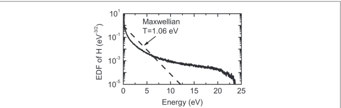
Figure8shows the atomic hydrogen energy distribution function in the center of the negative ion source for a 60kW absorbed power and 0.3Pa background gas pressure. The distribution function is highly non-Maxwellian and its properties are mostly controlled by the production and collisions ofHatoms against the walls of the ion source(the total mean-free-path is of the order of 1 m, i.e., signiﬁcantly larger than the dimensions of the device). Reactions which either generate (so-called source term) or remove (loss term) hydrogen atoms from the ion source volume are summarized in table4. Particle and power(gain or loss) are shown as a percentage of the total.Hatoms are mostly created and heated by the wall recombination of protons and molecular ions on the ion source walls(reaction #1 with 45 % of the particle production and 77 % of the energy gain) and by the volume dissociation ofH2(reaction #2).H+xions(where =x 1–3) are mainly generated

inside the discharge and are accelerated by the plasma potential toward the walls of the ion source. The amplitude of the potential in the driver is about 50 V for 60kW of RF power at 0.3Pa in the experiments [11]

Figure 8. Energy distribution function for atomic hydrogen in the center of the negative ion source. We implemented a 60kW absorbed power, 0.3Pa background gas pressure and no magnetic ﬁlter ﬁeld.

Table 4. Particle and power source(loss) terms for the production(destruction) of hydrogen atoms inside the ion source_{(60 kW absorbed power, 0.3 Pa, no magnetic} ﬁlter ﬁeld).

# Reaction Particles Power

Source terms 1 H+x  H(surface) 45.6% 77.2% 2 e+H2 e+ 2H 47.6% 19.6% 3 Other processes 6.8% 3.2% Loss terms 4 e+H 2e+H+ 14.2% 2.4% 5 H+H2 H+H2 — 3.6% 6 H H(surface) — 40.4% 7 H H2(surface) 85.8% 53.6%

(18)

and henceH+_xions impact the walls with a high energy. This explains the origin of the large energy tail in the distribution function of atomic hydrogen as shown inﬁgure8. Lastly,Hatoms loose most of their energy through collisions with the source walls(∼95%, reactions #6 and 7). TheHandH2temperatures are strongly

dependent on the assumptions that are made on the wall reactions(accommodation coefﬁcients provided in table3).

The energy distribution function for molecular hydrogen is shown inﬁgure9.H2molecules are created

uniquely through the recombination ofH+xions andHatoms on the walls. Molecular hydrogen is emitted from

the surfaces as a Maxwellianﬂux at Tw=300 K (where Twis the temperature of the surface). The energy

distribution function is wellﬁtted by a Maxwellian (up to about T6 H2). The mean-free-path is ∼10cm, i.e.,

smaller than the dimension of the ion source. The energy tail is induced by the collisions with the warmHatoms (TH1 eVfor 60kW and 0.3Pa while TH20.08eV). Molecular hydrogen is mainly heated through elastic

collisions with atoms(∼65% of power gain, reaction #1) and by electrons (reaction #2) as shown in table5. The calculations have been performed either with or without a magneticfilter field in the expansion chamber. The magnetized case corresponds to a maximumfield amplitude ofBmax=15Gclose to the PG, which is lower than thefield in the actual experiment (∼75 G on axis) but neverthelesshB=meB and the1 electrons are fully magnetized(a smaller magnetic field is used in the simulation because of numerical issues at the time with thefluid model for large magnetic fields). The indirect effect of the magnetic field on the neutral dynamics is that the depletion ofH2occurs in the area where the electron density is highest(i.e. in the driver

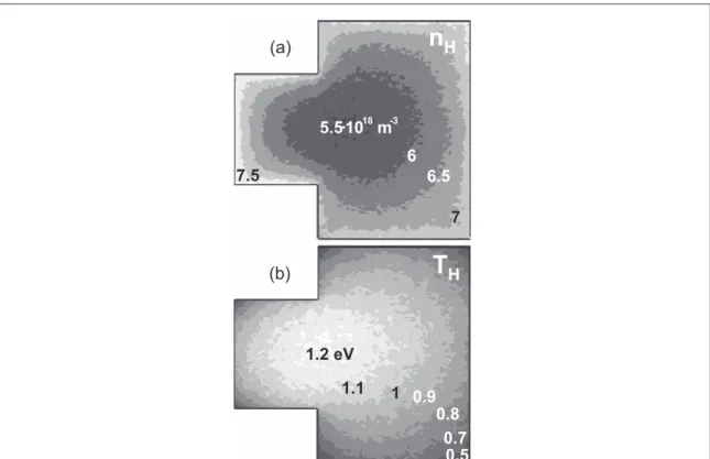
when the expansion chamber is magnetized) because molecular hydrogen is dissociated or ionized mainly by electrons(table5). The density proﬁle of hydrogen atoms is on the contrary quite insensitive to the magnetic

ﬁeld due to the fact that the volume losses (ionization) are signiﬁcantly smaller than forH2(i.e., ∼14% of the

total losses, see table4) and that the mean free path, ∼1m, greatly exceeds the ion source dimensions. The 2D

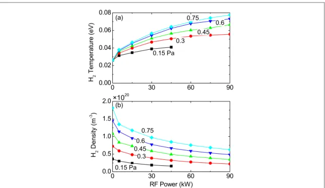
density and temperature proﬁles for theHatoms are shown inﬁgure10. Figure11displays the electron density and temperature averaged over the negative ion source volume versus the absorbed RF power in the discharge and the background gas pressure. For a pressure of 0.75Pa, the electron temperature is almost independent of the external power while the electron density increases quasi-linearly with power. This behavior may be

Figure 9. Energy distribution function for molecular hydrogen in the center of the negative ion source(60 kW absorbed power, 0.3 Pa, no magneticﬁlter ﬁeld).

Table 5. Particle and power source(loss) terms for the production(destruction) ofH2.

# Reaction Particles Power

Source terms 1 H+H2 H+ H2 — 66% 2 e+H2 e+ H2 — 13.7% 3 H+x H2(surface) 17.3% 1.4% 4 H H2(surface) 82.7% 6.7% 5 Other processes <0.1% 12.2% Loss terms 6 e+H2 e+2H 45.9% 6.4% 7 e+H2 2e+H+2 46.5% 6.5% 8 H2 H2(surface) — 85.9% 9 Other processes 7.2% 1.2%

(19)

explained by a global model. Assuming steady-state conditions, the total amount of particles created through ionization in the ion source volume at a given time is equal to the number of particles lost on the device walls,

= á ñ ( )

n u Ss B n k n V ,g i 24

where nsis the plasma density at the sheath edge, á ñn is the average plasma density(ne= niis assumed),

=

uB eT me iis the Bohm velocity, miis the mass ofH+2,k Ti( )e is the ionization rate(which is a function of the

Figure 10. Atomic hydrogen density(a) and temperature (b) proﬁles. 2D DSMC calculation withPabs=60kW, a background gas pressure of 0.3Pa,Bmax=15G and a PG bias voltage of 10V.

Figure 11. Electron density and temperature averaged over the ion source volume. 2D DSMC model for neutral transport, 2Dfluid model of the plasma without magneticfilter field.