Classification and modeling of forested terrain using LIDAR sensing

(1)

Classification and Modeling of Forested Terrain using LIDAR Sensing by

Matthew W. McDaniel B.S., Mechanical Engineering

B.S., Economics

Rensselaer Polytechnic Institute (2008)

Submitted to the Department of Mechanical Engineering in Partial Fulfillment of the Requirements for the Degree of

Master of Science in Mechanical Engineering at the

Massachusetts Institute of Technology September 2010

Signature of Author ………... Department of Mechanical Engineering August 6, 2010

Certified by ………... Karl Iagnemma Principal Research Scientist Thesis Supervisor

(2)

(3)

Classification and Modeling of Forested Terrain using LIDAR Sensing by

Matthew W. McDaniel

Submitted to the Department of Mechanical Engineering

on August 6, 2010 in Partial Fulfillment of the Requirements for the Degree of Master of Science in Mechanical Engineering

ABSTRACT

To operate autonomously, unmanned ground vehicles (UGVs) must be able to identify the load-bearing surface of the terrain (i.e. the ground) and obstacles. Current sensing techniques work well for structured environments such as urban areas, where the roads and obstacles are usually highly predictable and well-defined. However, autonomous navigation on forested terrain presents many new challenges due to the variability and lack of structure in natural environments.

This thesis presents a novel, robust approach for modeling the ground plane and main tree stems in forests, using 3-D point clouds sensed with LIDAR. Identification of the ground plane is done using a two stage approach. The first stage, a local height-based filter, discards most of the non-ground points. The second stage, based on a support vector machine (SVM) classifier, operates on a set of geometrically-defined features to identify which of the remaining points belong to the ground. Finally, a triangulated irregular network (TIN) is created from these points to model the ground plane.

Next, main stems are estimated using the results from the estimated ground plane. Candidate main stem data is selected by finding points that lie approximately 130cm above the ground. These points are then clustered using a linkage-based clustering technique. Finally, the stems are modeled by fitting the LIDAR data to 3-D geometric primitives (e.g. cylinders, cones).

Experimental results from five forested environments demonstrate the effectiveness of this approach. For ground plane estimation, the overall accuracy of classification was 86.28% and the mean error for the ground model was approximately 4.7 cm. For stem estimation, up to 50% of main stems could be accurately modeled using cones, with a root mean square diameter error of 13.2 cm.

(4)

(5)

Acknowledgements

I would like to thank my advisor, Karl Iagnemma, for his guidance in this research and for the opportunity to work on this project. I would also like to thank Takayuki Nishihata, Chris Brooks and Phil Salesses for their help with this work.

(6)

(7)

List of Figures

Figure 1.1: Connecting lower surface to possible ground points (from [16]). ... 15

Figure 1.2: Wrapped surface reconstruction using LIDAR data (from [26]). ... 19

Figure 1.3: Tree circle layers of 10 cm thickness (from [25]). ... 20

Figure 1.4: From left to right – segmented skeleton, voxel space, point cloud (from [27])... 21

Figure 2.1: Nodding device for collection of LIDAR data... 25

Figure 2.2: Hokuyo UTM-30LX scanning range finder... 27

Figure 2.3: MicroStrain 3DM-GX2 IMU. ... 28

Figure 2.4: Panoramic images of (a) baseline (b) sparse, (c) moderate, (d) dense1 and (e) dense2 scenes. ... 32

Figure 2.5: Hand-labeled point clouds of (a) baseline (b) sparse, (c) moderate, (d) dense1 and (e) dense2 scenes... 35

Figure 3.1: A portion of the Cartesian space partitioned into columns. ... 38

Figure 3.2: A column and its neighbors... 39

Figure 3.3: Pyramid filter visualization. ... 43

Figure 3.4: Ray tracing visualization. ... 44

Figure 3.5: Ground plane point cloud for baseline scene. ... 50

Figure 3.6: Ground plane point cloud for sparse scene. ... 50

Figure 3.7: Ground plane point cloud for moderate scene. ... 50

Figure 3.8: Ground plane point cloud for dense1 scene. ... 51

Figure 3.9: Ground plane point cloud for dense2 scene. ... 51

Figure 3.10: ROC curves for baseline, sparse, moderate, dense1 and dense2 scenes. ... 53

Figure 3.11: Delaunay triangulation. ... 55

Figure 3.12: Ground plane model for baseline scene using Delaunay triangulation... 56

Figure 3.13: Ground plane model for sparse scene using Delaunay triangulation... 56

Figure 3.14: Ground plane model for moderate scene using Delaunay triangulation. ... 56

Figure 3.15: Ground plane model for dense1 scene using Delaunay triangulation. ... 57

Figure 3.16: Ground plane model for dense2 scene using Delaunay triangulation. ... 57

Figure 4.1: Two consecutive horizontal LIDAR scan lines and height difference... 65

Figure 4.2: Hierarchical clustering example (from [42])... 68

Figure 4.3: Divide and conquer clustering example: initial data and center data... 72

Figure 4.4: Divide and conquer clustering example: column-scale clustering... 72

Figure 4.5: Divide and conquer clustering example: final clustering results. ... 73

Figure 4.6: Example overhead views for good cylinder/cone fits. ... 79

Figure 4.7: Bad ratio of radius to distance from cylinder center to distance centroid... 80

Figure 4.8: Bad ratio of diameter to maximum data spacing... 82

Figure 4.9: Cylinder position on wrong side of data. ... 84 Figure 4.10: RMS and median errors for cylinders and cones as a function of D130 slice width.

(10)

Figure 4.12: Linkage clustering results for baseline scene... 88

Figure 4.13: Linkage clustering results for sparse scene... 88

Figure 4.14: Linkage clustering results for moderate scene... 88

Figure 4.15: Linkage clustering results for dense1 scene... 89

Figure 4.16: Linkage clustering results for dense2 scene... 89

Figure 4.17: Cone and cylinder plots for baseline scene... 92

Figure 4.18: Cone and cylinder plots for sparse scene... 93

Figure 4.19: Cone and cylinder plots for moderate scene. ... 94

Figure 4.20: Cone and cylinder plots for dense1 scene. ... 95

Figure 4.21: Cone and cylinder plots for dense2 scene. ... 96

Figure 4.22: Stem estimation error as a function of range from the LIDAR... 98

Figure 4.23: 13 m Cutoff: RMS and median errors as a function of D130 slice width... 99

(11)

List of Tables

Table 2.1: Hokuyo UTM-30LX specifications... 26

Table 2.2: MicroStrain 3DM-GX2 specifications ... 27

Table 2.3: Elevation Change and Maximum Ground Slope ... 29

Table 2.4: Number of Trees in Experimental Test Scenes ... 30

Table 2.5: Summary of LIDAR data... 32

Table 3.1: Stage 1 Height Filter: Points Removed from baseline Scene... 45

Table 3.2: Stage 1 Height Filter: Points Removed from sparse Scene... 46

Table 3.3: Stage 1 Height Filter: Points Removed from moderate Scene ... 46

Table 3.4: Stage 1 Height Filter: Points Removed from dense1 Scene ... 46

Table 3.5: Stage 1 Height Filter: Points Removed from dense2 Scene ... 46

Table 3.6: Stage 1 Height Filter: Column Analysis... 47

Table 3.7: Stage 2 Classifier: baseline Scene ... 48

Table 3.8: Stage 2 Classifier: sparse Scene ... 48

Table 3.9: Stage 2 Classifier: moderate Scene ... 49

Table 3.10: Stage 2 Classifier: dense1 Scene ... 49

Table 3.11: Stage 2 Classifier: dense2 Scene ... 49

Table 3.12: Classifier Accuracy for Different SVM Thresholds... 54

Table 3.13: Mean and Median Ground Plane Error... 58

Table 4.1: Memory Profile of Computer Used for Matlab Computations... 70

Table 4.2: Clustering Results and Errors ... 90

Table 4.3: Number of Trees Successfully Modeled Using Cylinders and Cones... 97

Table 4.4: RMS and Median Diameter Errors Using Cylinders and Cones ... 100

Table 4.5: Mean Free Path for Final Cone Estimations... 103

Table 4.6: Species Groups (from [6]) ... 104

(12)

(13)

Chapter 1

Introduction

1.1 Problem Statement and Motivation

Unmanned ground vehicles have demonstrated effective autonomous operation in a variety of scenarios, including cross-country and urban environments [1-2]. Future applications for UGVs will require autonomous operation in forested environments. For UGVs to plan safe paths in forested environments, the systems will need to be able to identify contours of the load-bearing surface (i.e. the ground). This will enable the system to identify positive and negative obstacles, and assess the traversability of candidate paths. This thesis addresses the problem of identification of the ground and obstacles (i.e. main tree stems) in 3-D point clouds sensed using LIDAR.

Identification of the ground plane from point clouds is straightforward in many 2 1/2-D environments (e.g. the surface of Mars) where most of the sensed points lie on the load-bearing surface, or in urban environments where the road surface is nearly flat. This problem becomes more challenging in forested environments, where the surface of the ground is uneven, and trees and other vegetation occlude distant terrain.

Obstacle detection is also non-trivial in forested terrain. Environments are typically fully 3-D, due to overhanging canopy, and obstacles such as trees and shrubs can be highly variable in

(14)

classification and modeling. Similar to the ground plane estimation problem, incomplete data due to occlusion can also be a problem when identifying obstacles.

Methods for LIDAR data analysis in forested terrain have various applications in exploration and mapping. For example, stem locations can be used as inputs for simultaneous localization and mapping (SLAM) algorithms, which attempt to build a map of an unknown environment while keeping track of a UGVs current position [3]. Ground-based LIDAR data can also be correlated to aerial data to enhance UGV localization [4-5]. This would provide a more accurate and detailed portrayal of an environment, which could possibly be extrapolated to other regions using aerial data.

This work also has various applications in the domain of forestry. For example, stem diameters can be used to calculate biomass using allometric regression equations (e.g. [6-9]). Biomass refers to the mass of the portion of biological material (e.g. trees, shrubs, grass) which is found above the ground surface [6]. This is a critical variable in ecological and geoscience studies, which investigate the role of vegetation in the carbon cycle [10-11]. The traditional, manual methods of measuring biomass are expensive and could greatly benefit from automated sensing [7]. Knowledge of tree stems can also be used to characterize forest stand structure, which describes the size and number of main tree stems per unit area of forest [12-13].

Forest cleaning is another application for this work. Forest cleaning is a process of thinning a forest in order to improve growing conditions for the remaining trees in the forest. Currently most cleaning is done manually, but would benefit greatly from mechanizing due to the high cost of cleaning huge areas. Many areas of production (e.g. mining, agriculture, transportation of goods) already benefit from the use of autonomous or semi-autonomous vehicles, but such methods have not been employed in the cleaning domain because of the

(15)

difficulty of the problem. However, some researchers, particularly in Sweden, have made attempts to address this problem. They have thoroughly analyzed many of the problems and logistics of implementing an autonomous cleaning UGV, but have not implemented a working prototype [14-15].

1.2 Review of Ground Plane Estimation

Previous work on 3-D ground plane estimation can be grouped into techniques designed for airborne LIDAR (e.g. [16-17]) and techniques developed for LIDAR mounted on ground vehicles (e.g. [18-25]). Due to the difference in perspective, algorithms targeted towards airborne LIDAR may not be appropriate for implementation on ground-based LIDAR systems. However, some of the concepts may have utility in both problem domains.

In [16], a method is described for defining a digital terrain model (DTM) using airborne LIDAR data. The method first creates a surface below the LIDAR point cloud. This surface is then deformed upwards, such that it coincides with suspected ground points and spans surface objects that are not part of the ground, as illustrated in Figure 1.1.

(16)

In [17], airborne LIDAR data was used to create a DTM for natural terrain. They used a vertical histogram method in which data was binned according to height. A majority filter was then used to reduce noise, and the lowest points were classified as ground.

Other work has addressed ground plane estimation from UGV-mounted LIDAR data. In [18], ground plane estimation was accomplished through application of a Random Sample Consensus (RANSAC) algorithm [19]. RANSAC is a general method for fitting experimental data to a model. Classical fitting techniques use as much data as possible to obtain an initial solution, and then attempt to eliminate invalid data points. When using unfiltered data, such methods are computationally expensive and solutions can suffer from gross outliers. RANSAC takes an opposite approach by operating on as small of an initial data set as possible, and then enlarging the set with consistent data when possible. This typically results in substantial computational advantages.

An approach to ground plane estimation based on Markov Random Fields (MRFs) has been applied in environments with flat ground partially covered by vegetation [20]. Here, interacting MRFs are used to enforce assumptions of (a) ground height varying smoothly, (b) classes tending to cluster (e.g. patches of vegetation of a single type tend to be found together) and (c) vegetation of the same type generally having similar height.

The approach to ground plane estimation presented in [21] uses an octree framework to find best fit planes in each region in which the LIDAR point cloud density exceeds a pre-defined threshold. A merging process is then used to connect neighboring planes which have similar normal vectors. It was also proposed that classifications could be done based on plane attributes (i.e. area, gradient, etc.) [22].

(17)

In [23], LIDAR data is used to generate a DTM of the ground plane for rough terrain. An initial prediction of the ground is obtained by selecting the lowest LIDAR return in each 0.5 m x 0.5 m horizontal grid cell. Next, features are extracted from the LIDAR data, including the average height of the LIDAR points in each cell and the standard deviation from a plane fit to the data in each cell. Then, as the vehicle drives over each cell, the true ground height is measured. Machine learning is then used to improve future ground predictions. This feedback loop allows the system to learn and improve performance during autonomous navigation. This algorithm was implemented on an automated tractor platform and tested on “dirt roads and… varied vegetation often over a meter tall.” This methodology for estimating the ground plane is fairly similar to the approach presented in this thesis, except that this work in [23] was implemented on a moving platform. It is also difficult to compare results because this testing was done in agricultural environments (e.g. dirt roads and tall grass), rather than forests environments which have very different structure. For example, forests are fully 3-D due to overhanging canopy and more solid obstacles, such trees and shrubs, which usually cause significant occlusion.

A ground filtering approach which is closely related to the method described later in this thesis was presented as part of a 3-D object classifier in [24]. This approach operates on the assumption that the ground will be less steep than a pre-defined slope. Following this

assumption, for a candidate LIDAR data point to belong to the ground, a downward-oriented cone with vertex at the candidate point (with an included angle proportional to the pre-defined maximum ground slope) must be empty of other points. The method proposed in this thesis adopts a similar approach as part of a larger ground plane estimation framework.

(18)

obtain an estimation of the ground plane, a horizontal grid is created over the sample plot, with cell size of 0.5 m x 0.5 m resolution. For each cell, the point with the lowest height value is selected as a ground candidate. Several filters are then used to remove data points that are not part of the terrain. The first filter specifies the maximum value for the z-coordinate of the data, which was a predefined limit of 10 m above the height of the scanner. Another filter eliminated points within a downward-oriented cone with a vertex at the scanner center, similar to the method described above in [24]. The authors mention that these filters remove much of the non-ground data. They noted that they manually removed the remainder of the erroneous data in a 3-D point cloud viewer. The authors also state that this method does not work well on all terrain, and they must alter their parameters on sloped terrain. There were no quantitative results for the accuracy of this approach.

1.3 Review of Stem Estimation

Similar to ground plane estimation, previous work in stem estimation can be split into techniques used with airborne LIDAR (e.g. [8, 26]) and techniques for ground-based LIDAR (e.g. [25, 27-28]). There have also been attempts to use the strengths of both aerial and ground-based LIDAR to do stem estimation in [29]. This is useful because airborne data typically cannot detect most surfaces below the upper canopy (i.e. ground, main stems), while ground-based collection typically cannot detect the upper canopy.

In [8], airborne LIDAR data is used to create a coarse DTM of the ground plane, by selecting the lowest return within a local search window ranging from 1 m x 1 m to 5 m x 5 m. Trees are then identified using a height-scaled crown openness index (HSCOI), which is an index that is calculated by analyzing the penetration of LIDAR points through the canopy at

(19)

various heights. This method is used to pinpoint tree locations. Next, tree heights are found by calculating the difference of the maximum and minimum LIDAR returns in a local search window. Stem diameters are then calculated using allometric regression equations that are a function of tree height. This work benefited from the use of aerial LIDAR which senses many data points in the tree canopy, including points at the top of the crown. This makes it relatively easy to calculate tree height, which is rarely possible with ground-based LIDAR.

Airborne LIDAR was also used in [26] to model trees. The focus of this work was to perform surface reconstruction of canopy based on a surface wrapping procedure. This could be used for biomass estimation or inventory analysis. Though the authors used this method

specifically for canopy reconstruction, it could also be applied to stem reconstruction. Of course this would require LIDAR data on all surfaces of the stem (i.e. data taken from multiple

viewpoints). As such, this approach would not be applicable for static ground-based LIDAR collection, but could be used on a moving UGV platform. Figure 1.2 shows an example of this surface wrapping reconstruction for a single tree.

(20)

There are several approaches that address stem estimation from UGV-mounted LIDAR data. As discussed in the previous section, [25] estimates the ground plane using a local height-based filter, and then uses several pruning filters to increase accuracy. Next, 10 cm horizontal slices of LIDAR data, which range between 0 and 20 m above the ground, are analyzed. Each slice is modeled as a circle or circular arc, and compared to neighboring slices for quality of fit. The authors were able to use relatively thin slices because they had access to LIDAR data with very high resolution. The method also attempts to remove branch points by comparing canopy-level slices to sections of lower portions of the tree. This method appears to work well, but the results were not quantified or compared to any actual measured quantity (e.g. hand-measured stem diameters). It was also unclear whether they classified or clustered the initial tree data, or whether there were any bushes or shrubs near the trees. Figure 1.3 shows an example of the circular slices for a group of trees.

(21)

The work in [27] addresses the problem of determining the structure of tree stems using LIDAR data. Specifically, they find the subset of LIDAR data that belongs to each stem, so that each stem can be modeled (e.g. cylinder fitting). This problem is difficult because of gaps in the data due to occlusion, and noisy data that does not belong to any main branch (e.g. leaves and twigs). Since there is no natural way of expressing connectivity of individual data points, this problem was solved in the voxel domain instead of working with 3-D point clouds of LIDAR data. This makes it possible to establish connectivity rules based on connectivity of voxels. After converting to the voxel domain, gaps in the data are filled in, and isolated points (noise) were removed. Finally, a “skeleton” was created from the full voxel tree, which resulted in a tree (in the data structure sense). This made it relatively simple to identify individual stems of the tree, and the original LIDAR data points belonging to that stem. This appears to be a useful method; however results were only shown for one tree. There is also no indication of how accurate this method is, or how well it estimates stem diameter. Figure 1.4 shows a segmented skeleton, as well as segmentations in the voxel and point cloud domain for a single tree.

(22)

The approach in [28] used a ground-based pan-and-tilt LIDAR to do 3D modeling of trees in forests. This work benefited from very dense data. The LIDAR had 0.054° resolution, and each tree was scanned from four different positions such that data was obtained for the entire trunk surface. To estimate stem diameter, very thin (2 cm) slices of LIDAR data were extracted at various heights off the ground. The points in each slice were fit to a circle, with an iterative method to remove outliers (e.g. branch points). Since the slices were very thin, there were many circle estimates for each stem. To take advantage of this, a binning technique was implemented which only retained the lowest 10% of diameter estimates for each stem. This was done because the authors found that their estimates consistently overestimated diameter. These estimated diameters were compared to actual caliper measurements, and were consistently very accurate, usually within 1 or 2 cm of the caliper measurements. While results were very good, it is difficult to predict the robustness of this method in more challenging environments. For example, trees in these tests were almost perfectly straight and had few branches along lower portions of the stem. It was also mentioned that understory vegetation was chemically controlled, making the trees highly visible. Finally, in each scene, one out of the four scans was always manually removed. This was done to remove inconsistent data, usually caused by wind which made the trees move. While these experiments were clearly performed under controlled circumstances, some of the main ideas in this algorithm are still useful. For example, the use of very thin slices of LIDAR data is quite valuable when there is access to extremely dense data.

The work in [29] used the strengths of both aerial and ground-based LIDAR data to find locations of trees. This was done by computing the number of LIDAR returns in 1 m x 1 m x 1 m voxels, and then assessing the 3-D distribution of voxel data to determine the location of trees. Based on the distribution, allometric regression equations can be used to acquire data for the

(23)

forest’s biophysical variables such as biomass. While this method is useful for finding tree locations, no attempt was made to model the size of the trees. However, diameters could be estimated using allometric equations, similar to those used for estimating biomass based on 3-D distributions.

1.4 Contribution of this Thesis

This thesis presents a unified, robust approach for both ground plane identification and stem diameter estimation.

The ground plane is identified using a two-stage approach. The first stage is a local height-based filter, which was inspired by approaches such as [8, 16, 23, 25]. In this step, the lowest LIDAR return is selected for each 0.5 m x 0.5 m cell in a horizontal grid, which discards most of the points that lie above the ground plane. In the second stage, a set of eight

geometrically-defined features are computed for each of the remaining points. Then a support vector machine (SVM), which is trained on hand-labeled LIDAR data, operates on the eight computed features to identify which points belong to ground. This concept is similar to the approaches in [23] and [25], however the method presented in this thesis uses more features and benefits from the use of machine learning (an SVM), which was not used in [25]. Lastly, the classified ground points are used to create a triangulated irregular network (TIN) which models the ground plane.

Next, the main tree stems are estimated using the results obtained from the ground plane estimation. Candidate stem data is selected by taking a horizontal slice of LIDAR data centered at a height of 130 cm above the ground. This approach is similar to the techniques presented in

(24)

data, which allowed them to use thinner slices than is possible here. However, the method presented in this thesis is feasible for both dense and sparse data sets. This means that it will be usable for a broader range of different LIDAR sensors, and can model trees that are farther from the sensor (which consequently have sparse LIDAR returns). The second stage of the stem estimation algorithm clusters the candidate stem data in order to determine which points belong to the same stems. It does not appear that any approaches in the literature perform a similar step. Some works such as [27] appeared to use only one tree to test their algorithm, so this problem was probably not addressed. It is assumed that other methods used some sort of manual method to extract individual tree data. Finally, stem are modeled by fitting each cluster of LIDAR data to cylinders and cones, and physics-based constraints are introduced to determine the quality of these fits.

Experimental results from five different forested environments demonstrate the effectiveness of this approach. For these five experimental data sets, ground data can be classified with an overall accuracy of 86.28%. Furthermore, the ground plane can be modeled with a mean error of approximately 4.7 cm. Cones are more suitable than cylinders for accurately modeling main tree stem, and were shown to accurately model up to 50% of main stems in the five test sets, with a root mean square diameter error of 13.2 cm.

This thesis is divided into four chapters. Chapter 2 presents the experimental equipment and environments used to test these algorithms. Chapter 3 and 4 detail the proposed methods for ground plane estimation and stem estimation, respectively.

(25)

Chapter 2

Experimental Data Collection Hardware and

Methods

2.1 Equipment

To facilitate the collection of LIDAR data, a nodding device was constructed using a camera tripod with a sensor platform mounted on top. The sensors include a LIDAR, and an inertial measurement unit (IMU) for inertially referencing the data. A laptop was used to stream data from the sensors. During data collection, the axis of the nodding device was 0.55 m from the ground. Figure 2.1 shows a picture of this setup.

(26)

The LIDAR model used for these experiments was a Hokuyo UTM-30LX scanning range finder [30]. This sensor was chosen for its relatively light weight, and high resolution and

accuracy. For comparison, this Hokuyo LIDAR weighs about 0.37 kg, while its popular competitors, such as the SICK LMS-291 (weight of 4.5 kg [31]), are much heavier. (However, the SICK LMS-291 has a range of 80 m, compared to the 30 m range of the Hokuyo UTM-30LX.) Use of lightweight sensors will be especially relevant when these techniques are implemented on UGVs where minimizing payloads is essential. For example, a MobileRobots Pioneer 3-AT can carry a maximum payload of 12 kg [32]. High resolution is important because it results in denser point clouds and enables more detailed analysis. This advantage was

demonstrated in [28], where slices of data were 2 cm thick and still dense enough to allow reliable least-squares fits to circles. This LIDAR device has a USB interface and requires a 12 VDC power supply. During experimentation, the power was delivered by a Lithium Ion battery pack, which contained four 3200 mAh LIFEPO Li-Ion cells [33]. Each cell supplied a voltage of 3.2 V; thus, the entire pack supplied 12.8 V. These batteries were chosen for their high power density. Table 2.1 lists some of the relevant specifications of the Hokuyo LIDAR and Figure 2.2 shows a picture of this sensor.

Table 2.1: Hokuyo UTM-30LX specifications Angular Range: 270º

Angular Resolution: 0.25º Scan time: 25 msec/scan Range: 0.1-30 m Accuracy: • ±30 mm (0.1-10 m) • ±50 mm (10-30 m) Weight: ~370 g Size: 60 x 60 x 87 mm

(27)

Figure 2.2: Hokuyo UTM-30LX scanning range finder.

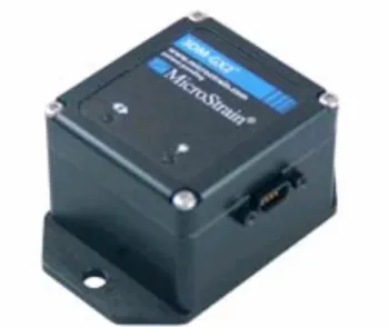
A MicroStrain 3DM-GX2 IMU was used in these experiments [34]. Similar to the Hokuyo LIDAR, this unit was chosen for its combination of relatively light weight and high accuracy. Table 2.2 lists some of the relevant specifications of the MicroStrain IMU and Figure 2.3 shows a picture of the IMU.

Table 2.2: MicroStrain 3DM-GX2 specifications Orientation Range: • Pitch: ±90º • Roll: ±180º • Yaw: ±180º Orientation Resolution: <0.1º Accuracy: • ±0.5º (static) • ±2.0º (dynamic) Weight: 39 g Size: 41 x 63 x 32 mm

(28)

Figure 2.3: MicroStrain 3DM-GX2 IMU.

2.2 Environments

LIDAR data was acquired for five different vegetated environments in the greater Boston area. In this thesis, these five data sets will be used to demonstrate the effectiveness of the classification and modeling techniques that are presented.

Three of the five data sets were collected in the summer of 2009. The first set of data,

baseline, was collected in Killian Court on the campus of MIT. This data is meant to be a

relatively simple baseline set that will be compared to the other, more complex scenes. A panoramic photo of this scene is shown in Figure 2.4(a). The two other data sets, sparse and

moderate, were collected at Harvard’s Arnold Arboretum, and panoramic images of these

environments are shown in Figure 2.4(b) and Figure 2.4(c), respectively. The sparse scene in Figure 2.4(b) contains several deciduous trees and shrubs, but is largely open. The moderate scene, shown in Figure 2.4(c), is more cluttered with numerous deciduous trees and shrubs, and significant ground cover.

(29)

The remaining two data sets, dense1 and dense2 were collected in January of 2010. Both of these sets were collected in Breakheart Reservation, which is located 9 miles north of MIT in Wakefield, Massachusetts. Panoramic images of these scenes, dense1 and dense2, are shown in Figure 2.4(d) and Figure 2.4(e), respectively. Both scenes contain significantly more deciduous trees than the previous data sets, and also have considerably sloped terrain. In the dense1 scene, there is a total elevation change of 4.2 m and the LIDAR is scanning down the hill. In the

dense2, the total change is 3.1 m and the LIDAR is scanning up the hill. Since both scenes were

collected during winter, there was snow on the ground and no leaf cover on deciduous trees. Table 2.3 shows the total elevation change and maximum slope of the ground for each of the five data sets. The maximum ground slope is computed by iterating though each hand-labeled ground point and comparing it to all other hand-labeled ground points that are at a distance greater than 1 m and less than 2 m away from the point. Each slope is also expressed in degrees from the horizontal.

Table 2.3: Elevation Change and Maximum Ground Slope

Scene Total Elevation Change Maximum Ground Slope

baseline 0.681 m 13.2°

sparse 1.784 m 18.0°

moderate 1.832 m 16.3°

dense1 4.202 m 24.1°

dense2 3.126 m 38.3°

These five sets were chosen with the intention of using amply diverse data to illustrate that the classification and modeling techniques in this thesis could be applied to a wide range of forested environments, and not just the test cases presented here. For example, in ground plane estimation, it is important to test algorithm performance on sloped terrain because it is a more

(30)

difficult problem than flat terrain. This was a recognized issue in [25], where inadequate ground plane results were obtained on sloped terrain.

Meanwhile, in stem estimation, many different trees and tree types should be tested. Trees can have vastly different size (height, stem diameter, etc.) and structure. For example, when trees have few branches along the main stem, they are relatively simple to model. However, a robust method should also work for trees that have more complex structure. Some methods in the literature use trivial cases with very straight and branchless trees [28], or use few trees to validate their algorithms [27].

There were various different tree types in the five experimental test scenes presented in this thesis. The baseline scene, collected at MIT in Killian Court, contained mature oak trees [35]. The trees in the sparse and moderate scenes from Arnold Arboretum included oak, beech, linden and lavalle cork trees [36]. The forests in Breakheart Reservation, where the dense1 and

dense2 scenes were collected, were primarily oak, hemlock and pine forests [37]. Among the

five scenes, there was also a large quantity of trees. Table 2.4 shows the number of trees in each scene.

Table 2.4: Number of Trees in Experimental Test Scenes

Scene Number of Trees

baseline 4 sparse 5 moderate 16 dense1 48 dense2 40 Total 113

The scene selection also incorporated seasonal variation due to the baseline, sparse and

(31)

collected in winter. This affects ground plane estimation because snow was on the ground in the winter scenes. In addition, there is less ground vegetation and no leaves on trees during winter. This affects the ground plane estimation problem because ground vegetation can occlude or be misclassified as ground. Likewise, canopy can occlude stems and be mistaken for main stem data by an algorithm. A robust algorithm should yield consistent results, even during different

seasons.

(a)

(b)

(c)

(32)

(e)

Figure 2.4: Panoramic images of (a) baseline (b) sparse, (c) moderate, (d) dense1 and (e) dense2 scenes.

2.3 Data Processing

As mentioned in Section 2.1, the Hokuyo LIDAR has an angular range of 270º and resolution of 0.25º. This means that in a single scan, the LIDAR collects 1081 points. Each of these points is the range associated with a given angle. Using an IMU to obtain the orientation of the LIDAR, all of these points can be transformed into an inertial frame where all of the points from a single scan lie in a single plane. Using the nodding device shown in Figure 2.1, the pitch of the LIDAR can be swept over a suitable range to obtain a point cloud of the environment. A summary of the data collected for the five scenes is shown in Table 2.5. Since the nodding device was operated by hand, there is some natural variation in the pitch range and number of scans across the data sets. Also, note that the number of data points is the maximum possible number of points. Some of these points may be null if the nearest surface in the line-of-sight of the LIDAR is out of range.

Table 2.5: Summary of LIDAR data

Scene Angular Range

(yaw) Pitch Range Number of Scans Total LIDAR data points

baseline 180º [-39º,+32º] 90 97,290

sparse 270º [-74º,+54º] 129 139,449

moderate 270º [-63º,+51º] 137 148,097

dense1 270º [-84º,+51º] 200 216,200

(33)

To quantify the accuracy of the algorithms presented in this thesis, the LIDAR data was hand-labeled using Quick Terrain Modeler software from Applied Imagery [38]. Each data point was classified into one of the four following categories:

1. Ground 2. Bushes/shrubs 3. Tree main stems 4. Tree canopy

In this work, the main stem is considered to be the “trunk” of the tree. Any stems branching off from the main stem are considered canopy. If a main stem splits into two or more stems, those multiple stems are considered canopy.

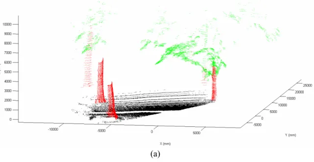
Figure 2.5 shows the hand-labeled LIDAR data projected into a global reference frame. Points are colored black, blue, red and green, representing ground, bushes/shrubs, tree main stems and tree canopy, respectively.

(34)

(b)

(35)

(d)

(e)

(36)

height of 130 cm above the ground) were measured using a tape measure. The estimated

diameter is then calculated for each tree, based on the assumption that the trees had round cross-sections. The diameter that is calculated from the measured circumference is considered the actual diameter of the tree, and this is compared to the diameter that is computed using the stem modeling algorithm.

All algorithms presented in this thesis were developed in Matlab. This was done for the purpose of quick implementation, thanks to the rich collection of toolboxes available in Matlab.

(37)

Chapter 3

Ground Plane Estimation

3.1 Overview of Approach

The approach proposed here divides the task of ground plane identification into two stages. The first stage is a local height-based filter, which encodes the fact that, in any vertical column, only the lowest point may belong to the ground. In practice this eliminates a large percentage of non-ground points from further consideration. The second stage is an SVM classifier, which combines eight heuristic features to determine which of the remaining points belong to the ground plane.

3.2 Proposed Approach

Given a set of LIDAR data points in Cartesian space, the goal of ground plane detection is to identify which of those points belong to the ground. In this work, candidate points are represented in an inertial frame with coordinates (x,y,z).

3.2.1 Stage 1: Height Filter

In the first stage, the points are divided into 0.5 m x 0.5 m columns based on their x and y values. These columns are identified by indices (i,j), where i=

_⎣

x/0.5

_⎦

and j=

_⎣

y/0.5

_⎦

. Thus,

(38)

highly unlikely that two points will identically share the minimum z value because every data point is saved with 1x10-4 mm precision. In the case that two points do share the minimum height, one will be chosen at random, and this will be based on the sorting of the minimum search algorithm in Matlab. This selection is acceptable because the entire ground plane is

computed on a 0.5 m x 0.5 m resolution. Thus, the location (in the X-Y plane) of the point within that column is a higher order effect. For simplicity, the lowest point in column (i,j) is hereafter denoted as a vector, Pi,j, with coordinates

[

xi,j,yi,j,zi,j

]

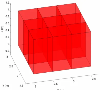
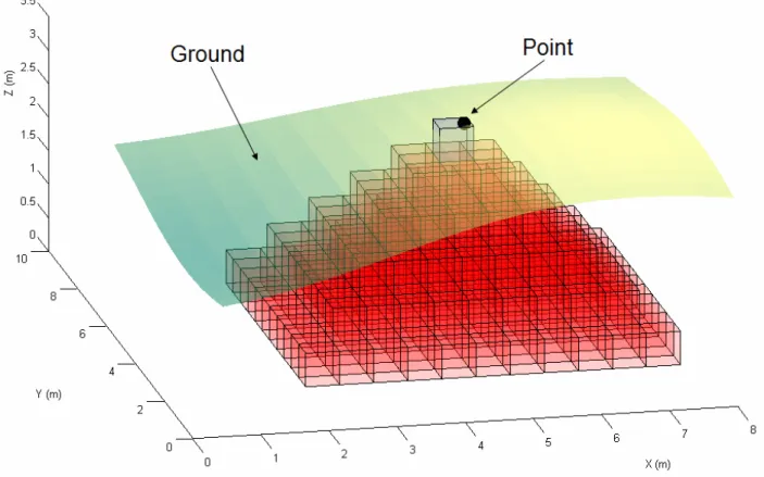
. Figure 3.1 clarifies the concept of

dividing the Cartesian space into columns.

Figure 3.1: A portion of the Cartesian space partitioned into columns.

3.2.2 Stage 2: Feature Extraction

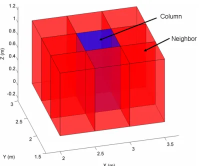
In the second stage of this approach, a variety of features are used to represent attributes of each point P_i,_j and the lowest points in each of the eight neighboring columns (i.e. P_i₋_1,_j₋₁,

(39)

Figure 3.2: A column and its neighbors.

A set of eight features was defined based on their usefulness in discriminating ground from non-ground. These features, denoted f1,…,f8 are combined into a feature vector

[

f1,..., f8

]

=

j i,

F for each point, which is used by a classifier to identify whether that point belongs to the ground. These features include:

• f1: Number of occupied columns in the neighborhood of column (i,j)

• f2: Minimum z of all neighbors minus zi,j

• f3: Value of zi,j

• f4: Average of all z values in neighborhood

• f5: Normal to best fit plane of points in neighborhood

• f6: Residual Sum of Squares (RSS) of best fit plane of points in neighborhood

(40)

These features are described in detail below.

f1: Number of occupied columns in neighborhood

The first feature, f1, is the number of occupied columns, N, in the neighborhood of

column (i,j):

f1 = N (3.1)

This feature is used to quantify the density of points around column (i,j). This encodes the fact that bushes, shrubs and tree trunks typically cast “shadows” in LIDAR data, thus reducing the number of occupied neighbors. As such, near bushes, shrubs and trees, not every column (i,j) will contain data points, so there will be no minimum in these columns. While this feature is useful, it will not be helpful in a column where the ground is occluded, but

overhanging canopy is still visible. The following features will address this case.

f2, f3, f4: Features using z height values

Feature f2 calculates the difference of zi,j and the minimum z of all neighboring columns:

(

zi j zi j zi j zi j zi j zi j zi j zi j

)

zi j

f₂ =min ₋₁_, ₋₁, ₋₁_, , ₋₁_, ₊₁, _, ₋₁, _, ₊₁, ₊₁_, ₋₁, ₊₁_, , ₊₁_, ₊₁ − _, (3.2)

This feature enforces the smoothness of the terrain around column (i,j). Intuitively, ground is expected to have a relatively smooth surface compared to the edges of trees or shrubs, which are expected to display larger changes in height. In the case of smooth ground, zi,j and the

minimum z of neighboring columns will be similar, and the difference will be small. This

difference will be larger when zi,j is an elevated point that is part of a tree or shrub, and one of its

(41)

Feature f3 is defined as the value of zi,j, and f4 is the average of all z values in the neighborhood of zi,j: j i z f₃ = _, (3.3)

(

z z z z z z z z z

)

N f4 = i−1,j−1 + i−1,j + i−1,j+1 + i,j−1+ i,j + i,j+1 + i+1,j−1 + i+1,j + i+1,j+1 / (3.4)

Features f3 and f4 utilize the z value (in the sensor frame) in each column. This enforces

the assumption that the ground will not be located significantly higher than the LIDAR sensor (i.e. the ground probably won’t be located at tree canopy height). This assumption is expected to be true except for cases with highly sloped terrain.

f5, f6: Features using best fit plane

For features f5 and f6, a best fit plane is calculated using all points in the neighborhood of

column (i,j). Given the set of N points in the neighborhood of column (i,j), where each point is denoted P , the mean is computed as: _k

∑

= = N k N 1 1 k P P (3.5)

The normal vector of the best-fit plane that minimizes orthogonal distances to the points in the neighborhood of column (i,j) is calculated as:

(

)

(

)

∑

= = ℜ ∈ ⋅ − = N k 1 2 1 , 2 3 min arg P P n n k n n j i, (3.6)

(42)

Feature f5 is the z-component of the unit normal vector, ni,j: ) 1 , 0 , 0 ( 5 =ni,j ⋅ f (3.7)

The z-component of this normal vector is expected to have a value near one for flat

ground. This is useful for discriminating between the ground and near-vertical structures, such as main tree stems and rock boundaries.

Feature f6 is the normalized orthogonal Residual Sum of Squares (RSS) of the best fit

plane:

(

)

(

)

∑

= ⋅ − = N k N f 1 2 6 1 j i, k P n P (3.8)

This is another feature to measure smoothness of the terrain around column (i,j), similar to feature f2. The ground is expected to be relatively smooth and thus lie nearly within the same

plane. Meanwhile, discontinuities will occur at the edges of trees or shrubs, and this will be reflected in a larger RSS of the best fit plane.

f7: Pyramid filter

A ground filter similar to the one described in [24] was also implemented. This technique assumes that the ground is unlikely to be steeper than a chosen pre-defined slope. Extending a ray downward (at a given slope) for every orientation in the X-Y plane will trace out a cone. Thus, in [24], this intuition was encoded using a downward-facing cone with its vertex coincident with the candidate ground point and the included angle corresponding to the pre-defined slope. For the candidate LIDAR point to belong to ground, that cone must be empty of other LIDAR points. In this work, a similar idea was used, but to improve computational

(43)

efficiency, the filter was discretized by forming a pyramid structure (instead of a cone) of cubic voxels under each point, P . The number of other minimum z points that fall within the pyramid _i,_j of P are counted, and this sum is used as feature f_i,_j 7. For this work, the maximum pre-defined

slope was set to one, which corresponds to an angle of 45° from the horizontal. As specified in Table 2.3, the maximum ground slope in the five test scenes is 38.3°, so a slope of one will yield the expected results. Figure 3.3 shows a pyramid of voxels under a candidate ground point, which is located in the blue voxel at the pyramid apex. Note that the ground surface is above all of the red voxels because the slope of the local ground is less than the slope of the pyramid.

(44)

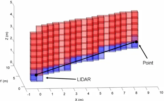
f8: Ray Tracing Score

The last feature is inspired by ray tracing. Intuitively, it is obvious that the ground (or any other structure) cannot lie directly between the LIDAR and any point it observes. Similarly, the ground cannot lie above the line segment formed between the LIDAR and any point it observes. Feature f8 quantifies this insight using a voxel-based approach. For each 0.5 m x 0.5 m x 0.5 m

cubic voxel containing a point, P , f_i,_j 8 is a sum of the number of line segments that pass through

a voxel in column (i,j) that is below the voxel that contains point P . Thus, points with lower _i,_j ray tracing scores are more likely to be ground, and points with higher scores are less likely. This concept is illustrated in Figure 3.4. The black arrow represents a ray traced from the LIDAR to a data point. The voxels that this ray passes through are blue, and the voxels above this ray are red. Any point in a red voxel would have its ray tracing score incremented by one.

(45)

3.2.3 Stage 2: SVM Classifier Description

Given the feature vectors Fi,j =

[

f1,..., f8

]

for all of the points in a training set and the

hand-identified labels of whether each point is ground, a SVM classifier is trained. Based on cross-validation within the training data, a set of appropriate kernel parameters can be found. (For this work, the SVM classifier was implemented using LIBSVM [39], and based on cross-validation, a linear kernel was used with SVM parameter C=100.) Using the trained classifier, points belonging to a previously unlabeled scene can be classified.

3.3 Experimental Results

The two-stage approach for identifying points on the ground plane was applied to the five experimental data sets described in Section 2.2 of this thesis, and the results are presented below.

3.3.1 Stage 1 Results

The results for the first stage of the ground plane estimation are presented in Tables 3.1-3.5. Each table shows the number and percentage of points that were removed using the local minimum z filter.

Table 3.1: Stage 1 Height Filter: Points Removed from baseline Scene

Label Initial Sensed

LIDAR Points Number of points after filter Percent of Points Removed Ground 53488 677 98.73 Bushes/Shrubs 0 0 -

Tree Main Stem 8324 26 99.69

Tree Canopy 7786 232 97.02

(46)

Table 3.2: Stage 1 Height Filter: Points Removed from sparse Scene

LIDAR Points Number of points after filter Percent of Points Removed Ground 74161 1131 98.47 Bushes/Shrubs 30987 463 98.51

Tree Canopy 32154 664 97.93

Total 141785 2305 98.37

Table 3.3: Stage 1 Height Filter: Points Removed from moderate Scene

LIDAR Points Number of points after filter Percent of Points Removed

Ground 65192 444 99.32

Bushes/Shrubs 67403 752 98.88

Tree Canopy 10314 379 96.33

Total 154403 1625 98.95

Table 3.4: Stage 1 Height Filter: Points Removed from dense1 Scene

Tree Canopy 10330 68 99.34

Total 112988 1521 98.65

Table 3.5: Stage 1 Height Filter: Points Removed from dense2 Scene

Tree Canopy 31919 89 99.72

(47)

This filter drastically reduces the number of points to be analyzed. It is important to note that each column in Cartesian space may contain many ground points, but only one minimum z point. Therefore, many ground points do get removed. Also, sometimes a higher fraction of ground points get removed than non-ground points, due to the fact that the ground near the LIDAR is scanned much more densely than trees and shrubs in the distance.

To assess the accuracy of this method, it is useful to analyze what types of points are in each column voxel. For example, columns that are farther away from the LIDAR may not have any ground points because the ground is occluded by trees and shrubs. However, if a column contains both ground and non-ground points, a ground point should be selected. These results are summarized in Table 3.6.

Table 3.6: Stage 1 Height Filter: Column Analysis

Scene Number of Points After Height Filter Columns with Only Ground Data Columns with Only Non-Ground Data Columns with Both and Ground was Selected Columns with Both and Non-Ground was Selected Accuracy of Columns with Both baseline 938 542 261 135 0 100% Sparse 2309 509 1174 622 4 99.35% moderate 1625 251 1176 193 5 97.41% dense1 1521 815 313 384 9 97.66% dense2 1574 694 352 521 7 98.66% Totals 7967 2811 3276 1855 25 98.65%

As expected, there are many columns in each scene where there are only non-ground points. However, in the columns with both ground and non-ground points, this filter stage selects ground points an average of 98.65% of the time.

(48)

3.3.2 Stage 2 Results

The second stage of this approach for ground plane identification uses an SVM classifier to assign each of the minimum z points as being ground or non-ground. The results are presented in Tables 3.7-3.11. For each data set, the SVM was trained using all other data sets. For example, the baseline scene was trained on the sparse, moderate, dense1 and dense2 scenes; the sparse scene was trained on the baseline, moderate, dense1 and dense2 scenes; etc. In the tables,

accuracy is calculated as the number of points correctly classified divided by the total number of points classified. Bushes, main stems and canopy classified as “non-ground” are considered to be classified correctly.

Table 3.7: Stage 2 Classifier: baseline Scene

Label Ground Non-Ground

Ground 666 11

Bushes/Shrubs 0 0

Tree Main Stem 10 16

Tree Canopy 0 232

Overall Accuracy 97.75%

Table 3.8: Stage 2 Classifier: sparse Scene

Ground 1032 99

Bushes/Shrubs 149 314

Tree Canopy 2 662

(49)

Table 3.9: Stage 2 Classifier: moderate Scene

Ground 441 3

Bushes/Shrubs 420 332

Tree Canopy 6 373

Table 3.10: Stage 2 Classifier: dense1 Scene

Ground 1131 68

Bushes/Shrubs 39 17

Tree Canopy 2 66

Table 3.11: Stage 2 Classifier: dense2 Scene

Ground 1077 138

Bushes/Shrubs 67 97

Tree Canopy 0 89

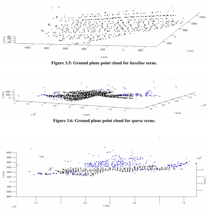
The results suggest that this classifier can effectively and consistently identify points belonging to the ground class. The average accuracy over the five data sets is 86.28%. It is helpful to visualize these results using point clouds. Figures 3.5-3.9 show the LIDAR data classified as ground by the SVM. This includes both true positives (i.e. ground points correctly classified as ground) and false positives (i.e. non-ground points incorrectly classified as ground). As with the plots in Section 2.3, points are colored black, blue, red and green, representing

(50)

ground points incorrectly classified as non-ground) are also plotted; each is marked with a black ‘X’.

Figure 3.5: Ground plane point cloud for baseline scene.

Figure 3.6: Ground plane point cloud for sparse scene.

(51)

Figure 3.8: Ground plane point cloud for dense1 scene.

Figure 3.9: Ground plane point cloud for dense2 scene.

The most inaccurate results were for the moderate scene, where classifier accuracy was only 72.55%. Looking at the classifier results (Tables 3.6 and 3.9) and the associated point cloud (Figure 3.7), it is easy to pinpoint the sources of errors. The primary issue was the significant ground cover immediately in front of the LIDAR. Since there were no ground points in these areas, bush/shrub points were selected for the minimum z filter. This can be verified by looking at Table 3.6. Compared to other scenes, there were relatively few columns in the moderate scene

(52)

columns that contained both ground and non-ground points. Since the ground cover was so low in this scene, bush/shrub data was frequently identified as ground by the SVM. From a physical perspective, this is reasonable because such low vegetation could probably be traversed by many UGVs.

These results also show that the proposed algorithm works well for sloped terrain. As shown in Table 2.3, both the dense1 and dense2 scenes have considerable slope, with maximum ground slopes of 24.1° and 38.3°, respectively, and total elevation changes of 4.2 m and 3.1 m, respectively. The point clouds in Figures 3.8 and 3.9 show that there were more true negatives at higher elevations. However, most of these points were near the edge of the sensor range where data is sparse and will be penalized by feature f1, which counts the number of occupied columns

in the neighborhood of column (i,j). Many high elevation points were still classified as ground, so a coarse ground plane model will still span these sparser sections.

If a lower rate of false positives is desired, the threshold of the SVM classifier can be adjusted. Figure 3.10 shows the receiver operating characteristic (ROC) curves for the five data sets.

(53)

Figure 3.10: ROC curves for baseline, sparse, moderate, dense1 and dense2 scenes.

With these results, fairly low false positive rates can be achieved while maintaining relatively high true positive rates. For example, for the baseline scene, a 70% true positive rate can be achieved with less than a 0.8% false positive rate. The same true positive rate could be achieved with less than 5% false positives for the sparse, moderate and dense1 scenes. The same true positive rate could be achieved with less than 10% false positives for the dense2 scene.

As suggested by the ROC curve, the threshold of the SVM can be tuned to classify a different number of points, depending on the user’s accuracy requirements. Changing the threshold effectively shifts the hyperplane that aims to separate ground points from non-ground

(54)

as many true positives as possible. Table 3.12 presents classifier accuracies for several shifts, where accuracy is calculated as the number of true positives divided by the sum of true positives and false positives. First, the accuracies are listed for the original classification results, which were presented in Tables 3.7-3.11. (Note that Tables 3.7-3.11 use a different accuracy metric.) The next column shifts the hyperplane, such that 80% of the true positives from the original classification remain on the same side of the hyperplane. In the last column, the hyperplane is shifted, such that 60% of the original true positives remain on the same side.

Table 3.12: Classifier Accuracy for Different SVM Thresholds

Classifier Accuracy (%)

Scene Original Classification 80% of Original True

Positives 60% of Original True Positives

baseline 98.52 99.44 100.00 sparse 86.36 93.33 97.48 moderate 49.89 78.10 91.10 dense1 94.09 97.94 99.13 dense2 92.61 96.96 99.23 average 84.90 94.38 98.01

As expected, when the hyperplane shifts to include fewer true positives, the accuracy improves because many of the original false positives change to false negatives.

3.4 Ground Plane Modeling

Following classification, the ground plane is modeled for each scene, using a triangulated irregular network (TIN).

3.4.1 Triangulation

(55)

triangulation finds triangles from a set of points such that no point in the set is inside the circumcircle (or circumsphere in 3-D) of any other triangle in the triangulation. To clarify this concept, Figure 3.11 shows an example of a Delaunay triangulation. The resulting triangles are shown with black lines and the circumcircles are gray. Note that no cimcumcircles contain the vertices of any other triangles.

Figure 3.11: Delaunay triangulation.

Delaunay triangulation was used to model the surface of the ground plane for each scene using the LIDAR data which was classified as ground by the SVM classifier in Section 3.3.2. Figures 3.12-3.16 show the resulting triangulation for each scene, where the color of each triangle is proportional to its height.

(56)

Figure 3.12: Ground plane model for baseline scene using Delaunay triangulation.

Figure 3.13: Ground plane model for sparse scene using Delaunay triangulation.

(57)

Figure 3.15: Ground plane model for dense1 scene using Delaunay triangulation.

Figure 3.16: Ground plane model for dense2 scene using Delaunay triangulation.

3.4.2 Ground Plane Accuracy

The accuracy of the ground plane model made out of Delaunay triangles is assessed by comparing the height of the ground plane model with the actual hand-labeled ground data. This

(58)

with any triangle, it is within range). The error is calculated by taking the difference of the height of the hand-labeled ground point and the height of the triangle at that same (x,y) position. Table 3.13 displays the mean and median errors for the five data sets.

Table 3.13: Mean and Median Ground Plane Error

Scene Mean Error (mm) Median Error (mm)

baseline 29.8 9.0 sparse 67.5 49.3 moderate 38.9 22.2 dense1 55.8 39.5 dense2 33.8 18.2 average 47.3 30.0

The largest errors are associated with the sparse and dense1 data sets. This is contrary to the classification results where the accuracies of the sparse and dense1 sets were better than the accuracies of the moderate and dense2 data sets. This occurred because, although fewer points were misclassified in these sets, the points that were classified incorrectly were farther from the ground plane.

Barring occlusion, there will always be some main stem and bush/shrub points that are connected to ground, but these points can also lie at higher elevations above the ground. Thus, misclassified main stem and bush/shrub points will have varying effects on the ground plane model. However, overhanging limbs (canopy data) will typically not be connected to the ground, and do tend to be higher above the ground plane. So misclassification of canopy data tends to have a more negative impact on the accuracy of the ground plane model. It is noted that only the

sparse, moderate and dense1 are the only three sets that misclassified any tree canopy data, and

(59)

Thus, assessing the accuracy of the ground plane model is valuable because it illuminates the fact that all classification errors do not affect the model equally. Physically, the ground plane error is low, with a total mean error of 47.3 mm and median error of 30.0 mm.

3.4.3 Ground Grid

The practical function of the ground plane model is to obtain the ground height, z, for a given (x,y) position in Cartesian space.

Recall that the first step of the ground plane estimation algorithm was a local height-based filter with a resolution of 0.5 m x 0.5 m in the X-Y plane. For this reason, it makes sense to discretize the ground plane model such that there is one ground height per 0.5 m x 0.5 m column that is contained within the bounds of the triangulation. Discretization is also

advantageous from a computational perspective because it only has to be calculated once, which avoids later duplicate computations. After it is calculated, ground height lookups are very fast.

The discretization is computed for each scene. In columns that contain a ground point from the classifier stage, the height of that point is used as the ground height in that column. In columns that do not contain a classified ground point but are within the bounds of the

triangulation, the height of the Delaunay triangle at the center of that column is used for the ground height.

The plane of the triangle, Ax+By+Cz =D, can be found by calculating the normal to that triangle. Given the points at the 3 corners of the triangle,

{

p1,p2,p3

}

, where each point is a vector pi =

[

xi,yi,zi

]

, the normal can be computed:

(60)

The last coefficient can be calculated using any one of the initial points, e.g.: 1 1 1 By Cz Ax D= + + (3.10)

The ground height at the center of the column can be found using the X-Y coordinates of the center of the column, (xc,yc), and solving for z in the plane equation:

(

D Ax By

)

C

z= − c − c / (3.11)

The above process essentially fills in gaps where there was not dense enough data to get classified ground points in every 0.5 m x 0.5 m column. This is the result of occlusion and greater range from the sensor. In these cases, there are large triangles which can span multiple columns.

Note that the ground will not be calculated for areas which are not within the bounds of the triangulation. This is acceptable because this only occurs at long ranges from the LIDAR. From a robotics perspective, it is essential that ground is modeled near the robot because this is necessary for immediate navigation. If it is desired, the robot can move closer to attain models of ground that is farther away.

3.5 Conclusions

This chapter has presented an approach for identifying ground points in 3-D LIDAR point clouds. This approach uses two stages. In the first stage, a local height-based filter

eliminates a large percentage of the non-ground points. In the second stage, a classifier operating on eight geometrically defined features identifies which of the remaining points belong to the ground. The proposed approach was experimentally validated using LIDAR data collected from

(61)

five forested environments. Results demonstrate that this approach can effectively discriminate between ground and non-ground points in such environments.

This ground plane estimation will be used as one of the inputs to the stem estimation in Chapter 4. Future work will involve extending this method to a moving vehicle. Ground plane estimation will be involved in the process of path planning for a UGV in a forested environment. Of course the accuracy of the final result would depend on the accuracy of mapping the data from the moving LIDAR into a stationary reference frame, which is a potential area for future research.

(62)

(63)

Chapter 4

Stem Estimation

4.1 Overview of Approach

The proposed approach models the main stems of trees (i.e. trunks) using basic 3-D geometric primitives (i.e. cylinder and cones). The first step of this process takes a horizontal slice of LIDAR data centered at a height of 130 cm off the ground. These points are then clustered, and fit to cylinders and cones. Finally, physical constraints are introduced to reject unrealistic fits.

4.2 Proposed Approach

The first step of main stem estimation is to identify which LIDAR data points belong to a single main stem (i.e. tree trunk). In this approach, candidate main stem data are chosen based on their height above the ground. This encodes the idea that at a certain height, stem data is likely to be above low lying vegetation and obstructions (e.g. shrubs, grass, rocks) and below higher vegetation (e.g. secondary stems and other canopy).

4.2.1 D130 Slice