Combining local and global optimization for planning and control in information space

Combining Local and Global Optimization for

Planning and Control in Information Space

by

Vu Anh Huynh

Submitted to the School of Engineering

MASSACHUSETTI OF TECHNC

SEP 0 5

LIBRA

in partial fulfillment of the requirements for the degree of

Master of Science in Computation for Design and Optimization

at the

MASSACHUSETTS INSTITUTE OF TECHNOLOGY

September 2008

@ Massachusetts Institute of Technology 2008. All rights reserved.

Author ý..% ...

...

...

School of Engineering

August 14, 2008

Certified by...

Nic~ Roy

Assistant Professor of Aeronautics and Astronautics

Thesis Supervisor

I

I

Accepted by...

_...

_.

_...

_Peraire...

Jaime Peraire

Professor of Aeronautics and Astronautics

Codirector, Computation for Design and Optimization Program

ARCHIV,'-6

S INSTITUTE OLOGY

Combining Local and Global Optimization for Planning and

Control in Information Space

by

Vu Anh Huynh

Submitted to the School of Engineering on August 14, 2008, in partial fulfillment of the

requirements for the degree of

Master of Science in Computation for Design and Optimization

Abstract

This thesis presents a novel algorithm, called the parametric optimized belief roadmap (POBRM), to address the problem of planning a trajectory for controlling a robot with imperfect state information under uncertainty. This question is formulated abstractly as a partially observable stochastic shortest path (POSSP) problem. We assume that the feature-based map of a region is available to assist the robot's decision-making.

The POBRM is a two-phase algorithm that combines local and global optimiza-tion. In an offline phase, we construct a belief graph by probabilistically sampling points around the features that potentially provide the robot with valuable informa-tion. Each edge of the belief graph stores two transfer functions to predict the cost and the conditional covariance matrix of a final state estimate if the robot follows this edge given an initial mean and covariance. In an online phase, a sub-optimal trajectory is found by the global Dijkstra's search algorithm, which ensures the balance between exploration and exploitation. Moreover, we use the iterative linear quadratic Gaus-sian algorithm (iLQG) to find a locally-feedback control policy in continuous state and control spaces to traverse the sub-optimal trajectory.

We show that, under some suitable technical assumptions, the error bound of a sub-optimal cost compared to the globally optimal cost can be obtained. The POBRM algorithm is not only robust to imperfect state information but also scalable to find a trajectory quickly in high-dimensional systems and environments. In addition, the POBRM algorithm is capable of answering multiple queries efficiently. We also demonstrate performance results by 2D simulation of a planar car and 3D simulation of an autonomous helicopter.

Thesis Supervisor: Nicholas Roy

Acknowledgments

This thesis could not have been completed without the support of numerous indi-viduals. I would like to thank my thesis advisor, Nicholas Roy, for his guidance and support. I gained a lot from every discussion we had.

My sincere gratitude goes to the CDO faculties and the fellow students in my class and research group. It is especially enjoyable to explore several research topics and have delicious food in weekly group meetings in CSAIL. I would also like to thank all the new friends I have made in MIT, who have made my life in MIT so wonderful.

I also gratefully acknowledge the generous financial support from the Singapore MIT Alliance.

Finally, I would like to thank my family for their unconditional love and encour-agement.

Contents

1 Introduction

1.1 M otivations ...

1.2 Problem statement and objectives . . . . 1.3 Approach and contributions . . . .

1.3.1 Approach ... 1.3.2 Contributions ... 1.4 Thesis outline ...

2 Literature Review and Problem Formulation

2.1 Sequential decision making . . . . 2.1.1

2.1.2

Markov decision process ...

Partially observable Markov decision proc 2.1.3 Exploration versus exploitation . . . 2.2 Advances in mobile robotics ...

2.3 Generic continuous-time problem . . . . 2.4 Approximated discrete-time problem . . . . 2.5 Statistical assumptions ...

2.6 Optimization problem ... 2.7 2D model of a planar car ...

2.7.1 Motion model ...

2.7.2 Feature-based map and sensor model 2.7.3 Cost model ... 2.8 3D model of a helicopter ... . . . . 22 ess ... 24 . . . . . 26 . . . . 27 . . . . . 28 . . . . . 30 . . . . 31 . . . . 33 . . . . 34 . . . . 34 . . . . . 35 . . . . 36 . . . . 37 15 . .. 15 . . . 16 . . . 17 .. . 17 .. . 18 .. . 18

2.8.1 M otion m odel ... 2.8.2 Sensor m odel ...

2.8.3 Cost m odel . . . .. . . . .

3 POBRM Algorithm

3.1 The framework of DP ... 3.1.1 Fully observable case ... 3.1.2 Partially observable case ... 3.2 Extended Kalman filter ...

3.3 iLQG algorithm ... .

3.4 POBRM: offline phase ... 3.4.1 Building a belief graph ...

3.4.2 Computing a locally-feedback control law for 3.4.3 Constructing covariance transfer functions . 3.4.4 Constructing cost transfer functions ... 3.5 POBRM: online phase ...

3.5.1 Sub-optimal trajectory ... 3.5.2 Sub-optimal controller ... 3.6 Sources of error ...

3.7 Analysis of the POBRM algorithm . ...

. . . . 44 . . . . . 46 . . . . 49 . . . . 53 . . . . 63 edge ... 66 . . . . . 68 . . . . . 70 . . . . 73 S... ... 74 . . . . 74

4 Experiments And Results 4.1 Performance of the iLQG algorithm 4.2 Performance of transfer functions . . . 4.2.1 Covariance transfer functions 4.2.2 Cost transfer functions... 4.3 Planning and control ... 4.4 Scalability to high-dimensional systems 4.4.1 Hovering ... 4.4.2 Landing ... 4.4.3 Navigating ... 83 . . . . . 83 . . . . . 85 . . . . . 85 . . . . 87 . . . . 88 . . . . . 9 1 . . . . 91 . . . . 92 . . . . 92 37 40 41 43 43

5 Conclusions 95

5.1 Summary ... . ... .... ... 95 5.2 Future directions ... ... 96

List of Figures

2-1 Graphical representation of an MDP (image courtesy of Nicholas Roy). 2-2 Graphical representation of a POMDP (image courtesy of Nicholas Roy). 2-3 System evolution of the considered problem as a POMDP . . . . . .

Car pose in the X-Y plane...

An example of a feature-based map . . .

Free body diagram of a quad-helicopter. The extended Kalman filter...

iLQG iteration. ...

Sampling a feature-based map... Belief graph ...

New query of the final covariance... Mechanism of covariance transfer function Illustration of the online phase . . . . .

. . . . 35 . . . . . 35 . . . . . 38 . . . . 50 . . . . 62 . . . . 66 . . . . 67 . . . . 69 s. ... 70 . . . . . 76

4-1 An example of iLQG trajectory ... 4-2 Profile of nominal controls ... 4-3 Estimated covariances v.s. fully updated covariances. 4-4 Running time to compute final covariances.. . . . . . 4-5 An example of an edge receiving many observations.. 4-6 4-7 4-8 4-9 Estimated cost values v.s. simulated cost values for Figure 4-5.. An example of an edge without any observation . . . . Estimated cost values v.s. simulated cost values for Figure 4-7.. No waypoint, cost value 16735 . . . . . 2-4 2-5 2-6 3-1 3-2 3-3 3-4 3-5 3-6 3-7 . . . . 84 . . . . 85 . . . . . 86 . . . . . 86 . . . . . 87 88 88 89 89

4-10 Three waypoints, cost value 340 ... .. . 90 4-11 An example of the hovering task. . ... . 91 4-12 An example of the landing task. . ... .. 92 4-13 A trajectory using the iLQG algorithm only with large covariances. . 93 4-14 A trajectory with the iLQG algorithm and the Dijkstra's search. . . . 94

List of Tables

4.1 An example of settings in an environment . ... 84 4.2 Comparing of unplanned and planned trajectory costs. ... . 90 4.3 Running time requirement for the offline and online phases... . 90

Chapter 1

Introduction

1.1

Motivations

Sequential decision-making is one of the central problems in artificial intelligence and control theory fields [19]. In domains where perfect knowledge of the state of an agent is available, a Markov decision process (MDP) is effective for modeling the interaction between an agent and a stochastic environment. Many algorithms have been studied extensively to find an optimal policy for a small-size to middle-size MDP [31 [29]. These algorithms often model state and control spaces as discrete spaces. However, in most real world problems such as robot navigation, the state of the agent is not fully observable at all times, in which case a partially observable Markov decision process (POMDP) is used to model interactions of the agent. In a POMDP, the system dynamics are known a priori, similar to an MDP, but the state of the agent must be inferred from the history of observations. The agent can maintain a distribution, called the agent's belief distribution, over states to summarize the entire history [19]. The problem of planning and controlling a robot with limited sensors is a challeng-ing question. In particular, flychalleng-ing unmanned aerial vehicles (UAVs) in GPS-denied environments such as indoor buildings or urban canyons has received increasing at-tention from research communities, industry and the military. With limited on-board sensors such as sonar ranging, laser ranging, and video imaging, UAVs acquire ob-servations to estimate their positions for decision-making and control. Moreover, the

states and control signals of UAVs are naturally in continuous spaces. Therefore, solving the problem of UAV navigation in this case inevitably leads to a complex continuous POMDP [30] [8].

Despite extensive research in recent years, finding an optimal policy in a POMDP is still a challenge for three main reasons. First, although we can convert a POMDP in state space to an MDP in belief space, available MDP algorithms for discretized belief space are computationally expensive even for small problems because the number of discretized belief states grows rapidly when agents interact with environments over time [19].

Second, an agent's policy must use available information to achieve the task at hand, which is known as exploitation, and, at the same time, take actions that further acquire more confidence in its state, which is known as exploration. Approximate approaches, such as certainty equivalence (CE), that use MDP algorithms to work on the means of state estimates instead of the entire belief space do not address well the balance between exploitation and exploration [33] [1].

Third, other attempts to use gradient-like algorithms with parameterized state and control spaces are often subject to local minima [19] [3] [29]. Most of current methods do not directly evaluate the quality of a sub-optimal solution, or the provided error bound is not tight enough [21]. Therefore, the error bound of a sub-optimal objective value compared to the globally optimal objective value still remains an open question.

1.2

Problem statement and objectives

In this research, we consider the problem of planning and controlling a robot to navigate from a starting location to a specific destination in a partially observable stochastic world. Abstractly, this problem can be considered as a partially observable stochastic shortest path (POSSP) problem [3] [4] [34]. The robot operates in envi-ronments where global localization information is unavailable. Instead, the robot is equipped with on-board sensors having limited range or field of view to estimate its

positions. Moreover, the robot is able to access to the feature-based map of an oper-ating environment. Each feature in the map is fully detected with known coordinates. In addition, the stochastic dynamics of the robot and sensors are given. Under these assumptions, our approach, the parametric optimized belief roadmap (POBRM), ad-dresses the above three difficulties to plan and control the robot directly in continuous

state and control spaces.

1.3

Approach and contributions

1.3.1

Approach

The POBRM is a two-phase algorithm, with an offline phase and an online phase. In the offline phase, we construct a belief graph by probabilistically sampling points around the features that potentially provide the robot with valuable information. Each edge of the belief graph stores two transfer functions to predict the cost and the conditional covariance matrix of a final state estimate if the robot follows this edge given an initial mean and covariance. The transfer function to predict the cost to traverse an edge is found by iterative stochastic algorithms, which are based on the least square curve-fitting method [4]. The transfer function to predict the conditional covariance of a final state estimate at an incoming vertex is based on the property that the covariance of the extended Kalman filter (EKF) can be factored, leading to a linear update in the belief representation [22] [8].

In the online phase, an approximation of an optimal trajectory is found by search-ing the belief graph ussearch-ing the global Dijkstra's search algorithm. We then refine the approximated trajectory using the iterative linear quadratic Gaussian algorithm (iLQG) and find a locally-feedback control policy in continuous state and control spaces [15]. Thus, the POBRM algorithm combines both local and global optimiza-tion in the offline and online phases to plan and control in belief space.

1.3.2

Contributions

The contributions of this thesis are three-fold. First, the POBRM algorithm aims at moving the computational burden of an induced optimization problem into the offline phase. The offline phase is computed only once for a particular map, and therefore it will save time in every online Dijkstra's search phase. In addition, the Dijkstra's search ensures the balance between exploration and exploitation. Compared to other approaches, the POBRM algorithm is not only robust to imperfect state information but also highly scalable to apply in high-dimensional systems and large-scale envi-ronments. Moreover, the POBRM algorithm is capable of answering multiple queries efficiently.

Second, we prove that if the belief graph contains edges along a globally optimal trajectory, by using the iLQG in the online phase, the error bound of a sub-optimal cost compared to the globally optimal cost can be obtained. Thus, in principle, the POBRM algorithm is able to provide a mechanism to evaluate the quality of a sub-optimal solution.

Third, to the best of our knowledge, it is the first time in this thesis that the problem of planning and controlling a six-degree-of-freedom helicopter with coastal

navigation trajectories [25] in continuous spaces is reported.

1.4

Thesis outline

The chapters of the thesis are organized as follows:

* Chapter 2 presents the overview of related work in artificial intelligence and control theory fields. This chapter introduces the fundamental of Markov de-cision processes in both fully observable and partially observable cases to solve this class of problems. In addition, the emphasis of exploitation and exploration in the partially observable case is presented. Also, related methods in dynamic programming (DP) such as iterative linear quadratic Gaussian (iLQG) are dis-cussed. Moreover, advances in mobile robotics, especially UAVs, are introduced.

This chapter also provides the mathematical formulation of the problem under consideration. An abstract framework with continuous-time and discrete-time formulations is presented first. Then, concrete system dynamics and sensor dynamics of a two-dimensional (2D) planar car and a three-dimensional (3D) helicopter follow.

* Chapter 3 discusses the POBRM algorithm. Most importantly, techniques in the offline phase and the online phase are developed in detail. In this chapter, we keep the algorithm in the most generic framework when presenting the iLQG algorithm to design a sub-optimal controller. When we start constructing a belief graph for a given feature-based map, we will focus more on the context of planning and controlling mobile robots. We then provide the preliminary theoretical analysis of the POBRM algorithm. We show that under suitable assumptions, the cost of a globally optimal trajectory can be bounded. The analysis in this chapter can serve as a theoretical basis for future work.

* Chapter 4 presents the results of experiments in simulation. In particular, 2D experiments simulate a mobile robot in a planar world, and the 3D experiments simulate a six-degree-of-freedom helicopter. Several results are shown to verify the theoretical results in Chapter 3.

* Chapter 5 discusses the main conclusions of this research. Also, several future research directions are suggested.

Chapter 2

Literature Review and Problem

Formulation

In this chapter, several important research concepts that are relevant to this work are presented. This review also sets the context for this work. To formulate the problem, we first state a generic continuous-time formulation, and then present the discrete-time approximation of the generic system. We next state additional assumptions to make the problem more tractable in this research, and give an induced optimization problem. Finally, we present the two-dimensional (2D) model of a planar car and the three-dimensional (3D) model of a helicopter.

2.1

Sequential decision making

Different research communities often address similar problems that arise indepen-dently in their fields. This is also the case for the problem of sequential decision mak-ing in artificial intelligence (AI) and control theory communities. In AI, researchers want to design an agent that can interact with an outside environment to maximize a long-term reward function. Traditionally, AI researchers often deal with discrete spaces in problems such as playing chess. Similarly, in control theory, researchers want to autonomously control a system in a certain environment to optimize some criteria. Researchers in this field often deal with continuous problems such as controlling a

mobile robot or guiding a missile [19].

Nevertheless, the above problems in AI and control theory share much in common. There are corresponding terminologies between Al and control theory. In particular, the terms agent, environment, and maximum reward in AI correspond respectively to controller, plant, and minimum cost in control theory [19]. In fact, recent research trends use techniques in both fields to address hard problems such as path planning

and control for a mobile robot. One of these techniques is based on dynamic program-ming from which a large variety of algorithms have been developed to address different characteristics of different problems. We will overview these techniques subsequently.

2.1.1

Markov decision process

Time

Figure 2-1: Graphical representation of an MDP (image courtesy of Nicholas Roy).

As mentioned in Chapter 1, a Markov decision process (MDP) is a common model of sequential decision making problems in both AI and control theory. An MDP is a model that specifies how an agent interacts with a stochastic environment with a known transition model. The components of an MDP are [24]:

* A set of states S, * A set of actions A,

* A set of transition probabilities T : SxAxS -+ [0, 1] s.t. T(s, a, s') = P(s'ls, a),

* A set of reward functions R : S x A -R,

* A discount factor y,

* An initial state so.

Figure 2-1 depicts graphically how these components relate with each other in an MDP. As can be seen here, at each state, the agent chooses an action, which results in a reward value and causes the state to change. The posterior state obeys the stochastic transition probability T. Furthermore, this figure also illustrates that the system is a first-order Markov graph. In other words, the distribution of a future state value depends only on the current state value and control input but not past state values and control inputs (Definition 2.1.1, 2.1.2).

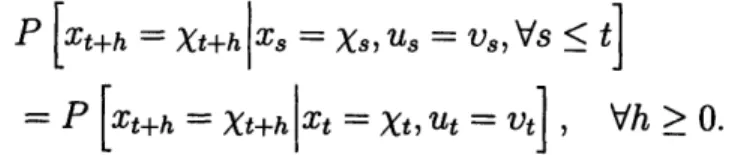
Definition 2.1.1. (Markov property) If x(t) and u(t) are two stochastic processes,

the Markov property states that, with x, X E S, and u E A,

P

[(t+h)

=

X(t+h) x(s)

=

(s), u(s) = v(s), Vs t]

=P[x(t+h)=x(t+h)x(t)=x(t),u(t) =u(t v(t)], Vh>0.

Definition 2.1.2. (Discrete-time Markov property) If Xk and Uk are two discrete

stochastic processes, the Markov property states that, with x, X E S, and u E A, P [Xt+h = _{Xt+hX = Xs, Us = v,Vs < t]}

=P[Xt+h= Xt+h zXt = t, Ut =Vt] , Vh>0.

Methods to solve an MDP are investigated extensively in [3] [29] [4]. Notable meth-ods are value iteration and policy iteration, which are based on Bellman's equation. The value iteration method iteratively finds the optimal objective values associated with possible states. From this value function, a suitable policy is then retrieved. Alternatively, the policy iteration method iteratively finds an optimal control policy

by evaluating the current policy and making policy improvements. Recently, Wang et al. have proposed a dual approach that explicitly maintains a representation of stationary distributions as opposed to value functions to solve an MDP [36] [35]. This yields novel dual forms of the value iteration and policy iteration.

2.1.2

Partially observable Markov decision process

]

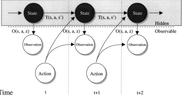
Figure 2-2: Graphical representation of a POMDP (image courtesy of Nicholas Roy).

Although an MDP is suitable for problems whose states are observable at all times such as playing chess, it is insufficient to model problems whose states are not directly observable. In such cases, a POMDP, which has additional observations, is suitable for modeling those problems [19] [24]. Components of a POMDP are:

* A set of states S,

* A set of actions A,

* A set of transition probabilities T : SxAxS S- [0, 1] s.t. T(s, a, s') = P(s'ls, a),

* A set of observation probabilities O : S x A x Z F [0, 1] s.t. O(s, a, z) =

P(zls, a),

* A set of reward functions R : S x Ax Z ý R,

* A discount factor y,

* An initial state distribution P(so).

Compared to an MDP, there are an addition set of observations Z and corresponding probabilities. Again, these components can be represented graphically in Figure 2-2. As can be seen, black states are inside the shaded box to denote that they cannot be directly accessed but must be inferred from the history of observations. Therefore, these states are called hidden states.

Methods that solve a POMDP with discrete states, discrete actions, and discrete observations are discussed in detail in [19] [30] [24]. The simplest approach is also based on Bellman's equation [30], which computes a sequence of value functions, for increasing planning horizons. At each horizon, the value function is represented as a piece-wise linear function, where the number of linear pieces increases rapidly with the horizon length. Point-based Value Iteration (PBVI) [21] [28] can be applied to prune unnecessary components. Using the PBVI method, Pineau et al. provide the error bound over multiple value updates, which depends on how dense the samples in the belief space are [21]. Kurniawati et al. have recently proposed a new point-based algorithm SARSOP, which stands for successive approximations of the reachable space under optimal policies [11]. This algorithm exploits the notion of optimally reachable belief space to compute efficiently.

To avoid the intractability of the exact POMDP value iteration, the belief space can be gridded using a fixed grid [17] [5] or a variable grid [6] [38]. Value backups are computed at grid points, and the gradient is ignored. The value of non-grid points are inferred using an interpolation rule.

There is a popular heuristic technique QMDP [16] that treats a POMDP as if it were fully observable and solves a related MDP. The QMDP algorithm can be effective

in some domains, but it will fail in domains where repeated information gathering is necessary. Heuristic search value iteration (HSVI) [27] is an approximate value iteration method that performs local updates based on upper and lower bounds of the optimal value function. Alternatively, forward search value iteration (FSVI) [26] is a heuristic method that utilizes the underlying MDP such that actions are chosen based on the optimal policy for the MDP, and then are applied to the belief space.

Other approaches employ approximation structures, including neural networks, to compute the value function or control policy for a subset of states and infer corre-sponding values for the rest of states [19]. Overall, these methods are computationally expensive.

Approaching from the local solution point of view, Li and Todorov have recently proposed the iLQG algorithm [13] [14] [15] to address the problem of control in partially observable environments, which can be regarded as a POMDP. The main idea of the iLQG algorithm is to find a sub-optimal control policy around the vicinity of some nominal trajectory instead of an optimal control policy for the entire state space. The nominal trajectory is iteratively refined to approach an optimal trajectory under some technical conditions. This method can provide a reasonable solution within an acceptable running time, which makes it attractive in real-time applications.

2.1.3

Exploration versus exploitation

The reason a POMDP is harder to solve than is an MDP is clearly because of the inaccessibility of the true state of a system. While an action in an MDP is chosen to maximize some reward function directly, an action in a POMDP balances two purposes: maximizing the reward function and gaining more confidence in its states. These two purposes were mentioned as exploitation and exploration in Chapter 1.

Tse et al. first mentioned the trade-off between exploitation and exploration in their series of papers in the 1970s [33] [1]. They called this the dual effects of caution (exploitation) and probing (exploration). On one hand, at any moment, if a controller focuses only on the current task, it will prefer a greedy way to achieve the task, but there will be a large uncertainty about accomplishing the task. On

the other hand, at any moment, if the controller focuses totally on gaining more confidence about its current state, the controller will seek actions providing more state information without accomplishing the current task. The optimal controller should balance between exploitation and exploration with the appropriate definition of an objective function. This balance has been examined by many others [29] [18], but as we will show in Chapter 3, in this research, we aim at balancing these two factors during the online phase of the POBRM algorithm with the assistance of the offline phase.

2.2

Advances in mobile robotics

The problem of making an autonomous mobile robot has been studied extensively by both AI and control theory control communities. Several fundamental methods, with many unique characteristics in the robotics field, are presented in [30]. Tradi-tional robot planning methods like the Probabilistic Roadmap (PRM) algorithm [10] assumes full accessibility of all parameters and dynamics of the robot and the envi-ronment. Since robots are becoming more and more autonomous but have limited sensors, such powerful accessibility is not always available.

In fact, controlling mobile robots in partially observable stochastic environments is still an on-going research topic. When maps are not available, the fundamental task is to determine the location of environmental features with a roving robot. This is called the simultaneous mapping and localization (SLAM) problem [30] [31]. With a given map, performing autonomous navigation is still challenging. Recently, Roy et al. [22] [8] [25] proposed the coastal navigation trajectories to make use of an available map to plan a set of waypoints to a destination. In their work, the main idea is inspired by the ship navigation in the ocean. That is, a ship should navigate along the coast to gain more confidence instead of taking the shortest trajectory with large uncertainty about reaching a destination. These methods can efficiently plan a sub-optimal trajectory even in large-scale environments. However, they only consider minimizing the final uncertainty at a destination but not consumed energy.

Furthermore, they do not provide a corresponding control law to follow this trajectory. In this thesis, we use a similar strategy to plan a sub-optimal trajectory, and at the same time, we provide a sub-optimal control law to follow this trajectory with more complex objective functions. Moreover, there is an important emerging research direction to learn all parameters and dynamics of robots and environments. This class of methods is within the regime of neuro-dynamic programming [4], or reinforcement learning [29]. In this research, although we assume robot dynamics and environments are given, we still apply some of these methodologies to learn part of the cost objective values.

Among many applications of autonomous robots, unmanned aerial vehicles (UAVs) have great potential. In particular, autonomous helicopters or quad-helicopters are useful in missions such as rescuing, monitoring, tracking due to their flexible flight dynamics and simple support infrastructure. Autonomous UAV flight in outdoor environments without GPS signals like forests is illustrated in [12]. It has been demonstrated that a controller can be designed to perform advanced and compli-cated maneuvers like inverted hovering [20]. The study of the flight dynamics of a quad-helicopter is presented in [9]. In this work, we show how the POBRM algorithm is applied in controlling a six-degree-of-freedom quad-helicopter with simplified flight dynamics in GPS-denied environments, as presented in Chapter 4.

2.3

Generic continuous-time problem

We consider a stationary continuous-time non-linear stochastic dynamic system gov-erned by the following ordinary differential equation (ODE):

dx(t) = f(x, u)dt + dw(t), (2.1)

where

* x(t) E X C RW

" is the state of the system and summarizes past information that is relevant for future optimization,

* u(t) E U C R~ n is the control input, or decision variable, to be optimized at any time instant t,

* w(t) E RIn is Brownian noise,

*

In the above system, the state x(t) is an element of a space X that represents state constraints. For instance, in the usual flight of a quad-helicopter, X is the set of poses with the pitch angle less than 60 degree. Similarly, the control u(t) is an element of a space U that is a set of admissible controls. It is worthwhile pointing out that states x satisfy the Markov property, which is mathematically stated in Definition 2.1.1.

Moreover, the state of the system is partially observable, and must be inferred from measured observations generated according to

y(t) = g(x) + (t), (2.2)

where

* y(t) E R₁ n _{is the measurement output of the system,} "* 9(t) E R", _{is Brownian noise,}

* g : R a -+ R' Y is a non-linear function of the state.

Eq. 2.2 represents one sensor model. If a robot has many different sensors, there are several models to describe these sensors.

We are interested in finding a feedback control law 7r* that minimizes the follow-ing objective function, also called the cost-to-go function, from startfollow-ing time 0 to unspecified final time T given an initial observation I(0) = y(O) of a starting state

x(0):

(I(0)) = E [h(x (T)) + T (t, x(t), r(t, I(t)) dt I(O) , (2.3)

7* = arg

min

where

* h(x(T)) is the final stage cost,

* £(t, x, u) is the instantaneous cost with control u(t) at state x(t),

* u(t) = 7r(t, I(t)), with 1(t) = {y(0..t), u(O..t-)},

* II is a set of admissible control laws 7r.

The conditional expectation is taken over the conditional distribution of x(0) given I(0), and noise processes w, t9. The information I(t) stores all measurements up to

and including the current measurement as well as all past control inputs. Using this information storage, a feedback control law 7r decides a control signal at the time instant t through u(t) = ir(t, I(t)). As this formula reads, this is a non-stationary control law that may vary with respect to time.

We can consider this problem as a partially observable stochastic shortest path problem (POSSP) in which we find a trajectory that minimizes the sum of traveling and terminating cost to final absorbing states. Due to stochastic environments, the shortest trajectory varies depending on the realizations of random factors in environ-ments.

2.4

Approximated discrete-time problem

The above continuous-time formulation captures the continuous nature of many en-gineering systems. However, in order to design optimal or sub-optimal control laws, the approximated discrete-time formulation is considered instead. In particular, each time step lasts A seconds, and thus the control horizon is N = . Eq. 2.1 and Eq.

2.2 can be approximated as:

Xk+1 Xk +f(k, Uk)A + WkVf, k = 0,1,..., N - 1

(2.5)

where Xk E X C

R

U

E

An information storage I(t) is also approximated as a vector Ik that stores sampled measurements and sampled control signals to design a feedback control law 7r:

Ik = [Yo, Y ... )Yk, UO, U0 , --., Uk-1] (2.7)

As discussed in Section 2.3, we want to find a feedback control law r that is non-stationary. Thus, a discrete time control law rx consists of N information-control mappings for N time steps:

7 = { P0, A1, ..., N-1}, (2.8)

Uk = [tk(Ik). (2.9)

Finally, the objective function and an optimal control law can be approximated by the formulae:

Jr(Io) = E h(XN) + Z k(Xk, k(1k)) I0 , (2.10)

k=0

7r* =arg mn J,(Io). _(2.11)

In Eq. 2.10, the integral of instantaneous cost over a duration A is approximated as

£k (Xkk (Ik)) =

e((k

k(Ik))A-2.5

Statistical assumptions

Before finding a solution to this problem, to make the system tractable, we consider the following statistical assumptions of Brownian noise processes w and V, and an

initial state xo:

* Wk and tk are independent of state Xk and control uk for all k,

* wk is independent of Ok for all k,

* Wks are i.i.d with a Gaussian distribution N(O, Qw),

" 9_{ks are i.i.d with a Gaussian distribution N(O, Qo),}

* x0 has a Gaussian distribution N(xzo, A), where x0 is a mean value.

These assumptions of independent Gaussian distributions enable rich probability ma-nipulations and inferences such as the Kalman filter and its variants [37]. In partic-ular, we only need means and covariances to describe these Gaussian distributions. Thus, they provide us with computationally feasible methods to handle probability density distributions over complex transformations.

I

4k-1

2.6

Optimization problem

With the above discussion, the problem under consideration can be expressed as the following constrained optimization problem:

minE h(N) + E (Xk, Uk) 0 (2.12)

k=O

subject to:

Xk+l =Xk + f(Xk, Uk)A + Wkvi, k = 0, 1, ..., N - 1 (2.13)

yk = g(xk)+ lk, k = 0, 1, ..., N (2.14)

Ik

=

[yO, Yl, ... , ,0, U1,

UOU...,) Uk-1],

(2.15)

Uk = IYk(Ik), (2.16)

7r = {A0o1, , .,, N-1}, (2.17)

xk E X C Rn,Uk EU C R"U, Yk E Rfn , _{wk E Rn,1 E k E IR,} n _(2.18)

wk e N(O, Q"), 9k N(0, •"), xo x N(xo, Ao), 1o = o. (2.19)

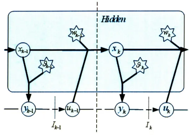
Figure 2-3 shows the evolution of this discrete-time system. As we can see, this structure resembles the well-known POMDP structure in literature. The nodes in the shaded rectangle are hidden states and noises, and the nodes outside this rectangle are the accessible measurements and control inputs.

This optimization problem is generally complex, and it is hard to find an optimal feedback control law to attain the minimum objective cost. Thus, in this research, we will look for a sub-optimal control law instead. Furthermore, we note that in this POSSP, the horizon N is unspecified. Nevertheless, for certain problems, we can exploit their structure to determine the horizon N heuristically, which we will show using the POBRM algorithm in Chapter 3.

2.7

2D model of a planar car

In this subsection, we discuss the concrete model of a planar car, which provides the dynamics and measurements of the car by a continuous-time formulation in Section 2.3. The content in this subsection is presented in detail in [30). Thus, the brief and simplified motion and sensor models are presented here.

2.7.1

Motion model

The pose of the car, consisting of an x-y location and a heading 0, operating in a plane, is depicted in Figure 2-4. We regard the pose information of the car as the system state:

x(t)

=

(2.20)

The control input for the car has two components, namely a translational velocity v and a rotational velocity w:

u(t) = (2.21)

We can have additional constraints to restrict these velocities in a certain range U: u(t)E U.

When applying a control u(t) to a state x(t), the system follows the following dynamics:

d(x(t)) = f(x, u)dt + dw(t) (2.22)

v cos(0)

A-Aul

x

Figure 2-4: Car pose in the X-Y plane.

2.7.2

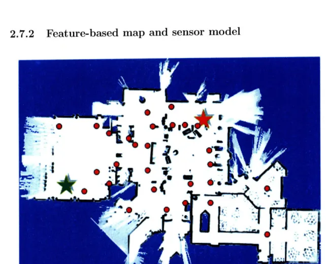
Feature-based map and sensor model

AIsh

C,

wIiaI,-i

IL

I A

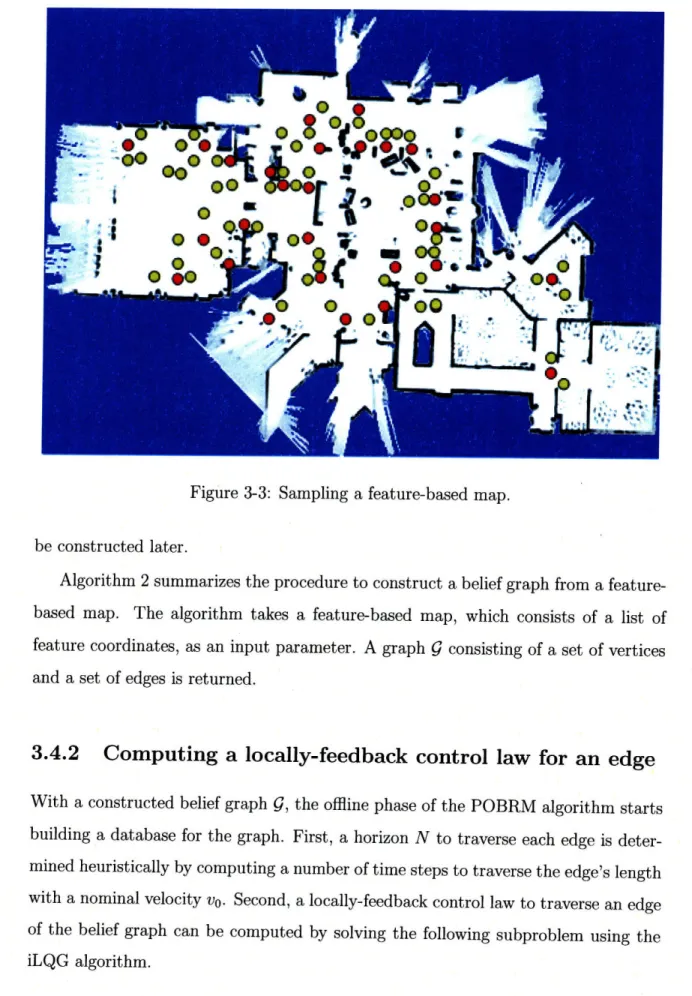
Figure 2-5: An example of a feature-based map.

[t.4i

sI

.e .00-1 ₀

Figure 2-5 shows an example of the typical map of an area in which the car may operate. Black objects are obstacles, and red dots are landmarks, or features. The green star is a starting location, and the red star is a destination. The area contains rich information for the car such as corners of buildings, walls, doors, and windows. These objects are called landmarks in a feature-based map. With a given feature-based map, the POBRM algorithm will exploit the map structure to solve the optimization problem in Section 2.6.

The car is equipped with sensors to work in the area. For a certain landmark locating at [mX my]T in that area, the car can sense the distance and relative bearing

to the landmark if it is within the visibility region of the car. We assume that when the car senses the landmark, it knows the landmark's coordinates. Depending on the car's location, at any instant of time, the car can receive no measurement, or a list different measurements from several landmarks. The measurement model is described

by

if (m - x)2 + (m - y)2 R (2.24)

y(t, m) = g(x, m) + V(t)

(2.25)

(mx -

X)

₊

_{(my- y)}

1

_(2.26)

atan2(my

-

y, mX -

x)

- 0

where Rm is the range of visibility of the car for that landmark.

2.7.3

Cost model

We want to find an optimal trajectory from a starting location to a destination with the final state ZG. The final stage cost function and instantaneous cost function are

h(x(T)) = (x(T) - XG)TQ(T)(X(T) - XG), (2.27)

£(t, x(t), u(t)) = u(t)TR(t)u(t), (2.28)

The weight matrices Q(T), R(t) are symmetric positive definite. Using these cost functions, we penalize large deviations from the final state Xe and prefer trajectories

with low energy consumption that reach the destination. Moreover, there is a trade-off between these cost components by setting different weight matrices Q(T) and

R(t).

2.8

3D model of a helicopter

In this subsection, we show how the optimization problem in Section 2.6 can be used to control the simplified dynamics and measurements of a six-degree-of-freedom (6-DOF) helicopter. For other complex models of aerospace vehicles and quad-helicopters, readers can refer to [39] and [9].

2.8.1

Motion model

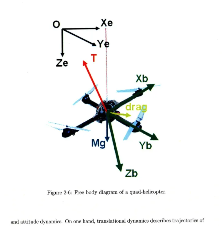
To define the dynamics of the helicopter, we have to work in the North-East-Down (NED) inertial coordinate system, and the body coordinate system, as shown in Figure 2-6. The NED coordinate system embeds its XE and YE axes into a horizontal plane and points ZE axis downward according to the right hand side rule with the fixed origin. The body coordinate system is aligned with the helicopter triad with the origin at the center of gravity (COG) of the vehicle. The XB axis points through the noise of the vehicle, and the YB axis points out to the right of the XB axis. Finally, the ZB axis pointing downward completes the coordinate system.

The x-y-z locations are defined in the NED coordinate system, while the yaw V, pitch 0, and roll q angles are defined as rotational angles from the NED coordinate system to the body coordinate system. We define the state of the helicopter as follows:

x(t)= x y z t y V) 0 0 (2.30)

where [ jy i]T is the velocity of the helicopter.

O

Xe

T

Ze

V

IXb

Figure 2-6: Free body diagram of a quad-helicopter.

and attitude dynamics. On one hand, translational dynamics describes trajectories of

x - y - z points under external forces as recorded by an observer. The Newton's law is a key tool to obtain translational dynamics. On the other hand, attitude dynamics describes how the vehicle rotates under external forces. The Euler's law is a main tool to obtain the dynamics of Euler angles 0, 0, and 0.

In this research, to keep the model simple, we assume that angle velocity can be controlled directly. Thus, we concern only with the Newton's law but not the Euler's law under external forces. Moreover, we also assume that the thrust generated does not depend on voltage power left on the helicopter. The control input is expressed as

follows

u(t)= [T T t

(2.31)

(2.32)

T > Tmin > 0,

where T is nonnegative thrust with minimum thrust Tin,

[

velocity. The transform matrix to rotate from the body coordinate system to the NED coordinate system is given by

[T]EB _{= [-V]zB [-0]YB [-1]XB}

cos -sin 0 cos 0 0 sin 0 1

= sin) cos 0 0 1 0 0 0 0 1 -sin0 0 cos0 0

cos 0 cos 0 - sin V cos 0 + cos 0 sin 0 sin 0 = sin 0 cos 0 cos 0 cos 0 + sin b sin 0 sin q

- sin 0

cos 8 sin 0

0 cos ¢ sin

0

q

cos

J

sin ' sin 0 + cos ' sin 8 cos

-cos o sin + sin o sin 8 cos

cos 0 cos

J

(2.35)

As shown in Figure 2-6, given M is the weight of the helicopter, we assume that an applied thrust is perpendicular to the helicopter body plane going through its COG. In addition, the velocity of the helicopter is small enough so that the drag force is proportional by a coefficient k and in an opposite direction to the translational velocity of the helicopter. By the Newton's law, we have:

[T]EB

0

T +

0

Mg - k

=

M

T(- sin

4

4-

4

]

T(cos 0 sin 0 - sin 0 sin 0 cos ) + -k = M

-T cos O

cos 0

Mg

- ki

MJ

(2.36)

T (- sin i sin -- cos i sin 0 cos q) - -i

T (Cos V sin $ - sin sin 0 cos ) -)

Scos

0 cos 0-

+

g

Thus, the helicopter dynamics are described by

d(x(t)) = f(x, u)dt + dw(t)

y

T (- sin sin ¢ cos sin 0 cos )

-S(cos

V sin ¢

-

sin sin 0 cos

b)

-

-L

dt + dw(t).

2.8.2

Sensor model

Similar to the 2D case, the feature-based map of an operating area is given. The helicopter is equipped with sensors to measure a distance to a landmark, and its translational velocity when the landmark is within its visibility. Moreover, as the pitch and roll angles are local knowledge of the helicopter, we assume that the heli-copter can sense the pitch and roll angles at any time using gravity and a three-axis accelerometer. In addition, we assume that the helicopter can estimate the yaw angle. These two components of measurement are described by

if

V(m•-

x)2 + (my -y)2 + (m~z- )2<

Rm:

(2.38)

v/(Mx -

x)I

+ (m - y) + (z

-

z)

0

+

(t),

(2.46)

2.8.3

Cost

model

Similar to the 2D car, we also find an optimal path from a starting location to a destination with the final state ZG. The final stage cost function and instantaneous

cost function are

h(x(T)) = (x(T) - G )TQ(T)(x(T) - XG), (2.47)

£(t, x(t), u(t)) u(t)TR(t))u(t), (2.48)

Chapter 3

POBRM Algorithm

In this chapter, we discuss in detail how to solve the optimization problem defined by Eq. 2.12 to Eq. 2.19 in Section 2.6. We start with the framework of dynamic programming (DP). The overview of the extended Kalman filter follows. Then, the iterative Linear Quadratic Gaussian (iLQG) algorithm is presented. After that, the offline and online phases of the POBRM algorithm are discussed. We attempt to provide a preliminary analysis of the POBRM algorithm. There are several sources of error that affect the accuracy of a returned sub-optimal solution. Next, we argue that, under special assumptions, it is possible to bound the optimal solution.

3.1

The framework of DP

The basic framework of dynamic programming, in which decisions are made in stages, is well studied in [3]. We notice that the formulated POSSP in Section 2.6 has a suitable structure to be solved by DP. The world of DP related algorithms such as MDP, POMDP, and Neuro-DP, as reviewed in Chapter 2, is vast. Hereafter, the usual case of fully observable DP is presented, and the extended partially observable DP follows.

3.1.1

Fully observable case

The decision making problem in a fully observable environment is described by

min E h(xN) + E k(Xk, Uk) XO

(3.1)

X

U

R•

_wkE

_(3.5)

The notations in Eq. 3.1 to Eq. 3.6 have the same meanings as their counterparts in Eq. 2.12 to Eq. 2.19. However, this formulation is much simpler as it formulates an MDP. First, all states of the system are directly accessible, thus no measurement output is needed. Second, an admissible feedback control input at any instant of time is a function of a state. Third, an objective function is evaluated given an observable starting state.

The DP framework is based on the following lemma called the principle of opti-mality proposed by Bellman.

Lemma 3.1.1. (Principle of optimality [3]) Let 7* = {J*,

j*,

E h(xN) + E k(Xk, Uk) XiI

k=i

Proof. Since ir* is an optimal policy, the cost objective J* induced by lr* is the

small-est. If the truncated policy is not optimal for the subproblem, let

{p

}

be an optimal sub-policy. Then the new policy ',' = {pi, D, ..., i4_-1~ A, A4,) ..., 7A_-1}

yields a smaller value of the original objective function than J*, which is a

contradic-tion. 0

Using Lemma 3.1.1, it can be proved by induction that the optimal cost for the basic fully observable DP problem can be computed backward as in the following theorem [3]: Theorem 3.1.1. Denote: N-1 J,(xo) = E h(xN) + fk(X k,Uk) k=0 J*(xo) = Jr-.(o).

For every initial state xo, the optimal cost J*(xo) is equal to Jo(xo), which is given by the following formulas for k from N - 1 down-to 0:

JN(XN) = h(xN), (3.7)

Jk(k) = min E [ek(Xk,uk)+ Jk+1(k+1) kk] , k = N- 1, N- 2,..., 1, 0.

(3.8)

Furthermore, let u* be a minimizer of the Eq. 3.8, and we assign IU*(xk) = u* for every Xk and k, then the policy lr* =

{p/,

In Eq. 3.8, we have a minimization problem over a feasible set Uk(xk), which is a subset of U. This feasible set depends on the current state xk because only control

3.1.2

Partially observable case

Let us turn our attention back to the DP framework in a partially observable envi-ronment. For the purpose of clarity, we restate the formulation here:

min E h(XN) + : ek(Xk, Uk) Io (3.9) k=0

subject to:

Xk+l = Xk + f(Xk, Uk)A + WkVA, k = 0, 1,..., N - 1 (3.10)

Yk = g(xk) + ?k, k = 0, 2,..., N (3.11)

Ik

=

[YO,

Y1,

...

,

Yk,

0

U

₁

*,

Uk-],

(3.12)

Uk = IAk(Ik), (3.13)

1 = {07, ,--, .7 N-1}, (3.14)

Xk -X CE RXnx, Uk U C R]nu, YkE Rn

o, Wk E Rn-, Ok E R•n, (3.15)

Wk - N(0, I•), 'Ok , N(0, 7Q), xo , N(xo, Ao), Io = YO. (3.16)

The Theorem 3.1.1 cannot be applied directly to this formulation due to the inaccessibility of states x. However, it is possible to reformulate the problem to become fully observable with respect to new information states I, control inputs u, and random disturbances y:

10 = YO, (3.17)

Ik+ = [Ik, uk, k+1], k = 1, 2, ..., N - 1. (3.18)

To see this, we first show that Ik satisfies the Markov property.

Lemma 3.1.2. With the dynamics of variables as defined in Eq. 3.9 to Eq. 3.18, the

Proof. From Eq. 3.18, we note that Ik is part of Ik+1 for all k, thus

P [Ik-1, Uk-1, *.. , ₀U k, Uk, ..**, I0, o] =1.

Therefore the following conditional probability holds:

P [Ik uk, Yk+1 Ik, Uk]

U0] =

P [Ik-1, Uk-1, - Io, uo0Ik, Uk, ... , IO UO]

= P [Ik, UYk+ 1Ik, Uk]

Again, From the dynamics of Ik+1 in Eq. 3.18, it follows that

P [Ik+1 Ik, k]

Corollary 3.1.1. Let X be any random variable:

E [XII ,

= E [XI]

,

forj < i.

This corollary states that the expectation of a random variable depends only on the current information vector but not past information vectors.

have the following facts:

Fact 3.1.1. Two common iterative expectation rules:

* Let X, Y, Z be random variables:

Furthermore, we

E[XY]

= E

[E[XIY•,

Z] Y].

* Let X, Y, Z be random variables:

E

[E[XIY]

_{+ Z Y]=}

E[X+ZY].

ZY

P [Ik, Uk, yk+1 ,u, ... 7

Uk

(3.20)

-Using these corollary and facts, the following theorem shows how the DP frame-work frame-works in a partially observable environment.

Theorem 3.1.2. Denote:

J(lo) = E h(XN)

+

E

£k

(k) Uk) I10

J*(Io) = 4J(lo).

For every initial information Io, the optimal cost J*(Io) is equal to Jo(Io), which is given by the following formulas for k from N - 1 down-to 0:

JN(IN) = EN [h(xN) IN] , (3.21)

Jk(Ik) = _Uk min Exk,k,yk+l _EUk(Ik) k (k, k) + Jk+1 (Ik+) Ik,

k

N

Furthermore, let u* be a minimizer of the Eq. 3.22, and we assign tL*(Ik) = u4 for

every Ik and k, then the policy lr* = {I*, ..., * N-1 } is optimal.

Proof. First, we rewrite the objective function in terms of information state Ik as in

a fully observable case:

N-1

Jr(Io) = Exo,Xl..N h(xg) + E fk(Xk, uk k)10

(3.23)

i=0

= EII..N EXN

[hN(XN)

I

i=0

= EIN..Nh(I hNkN + ksi(I 7k 0 (3.25)

i=0

where the first equality is obtained using the iterative expectation rule in Fact 3.19 and reducing the inner conditional expectation using the Markov property in Corollary

3.1.1 with shorthands:

hN(IN)

=

EXN [hN(N)II

N]

(3.26)

k (Ik, k) = Ex,

[k (k,

Uk)l

,

(3.27)

Therefore, now we can express the cost function as the newly set-up fully observable system:

N-1

J,(Io) = EIl..N h(I) + Ik, Uk)Io (3.28)

i=0

Hence, the DP framework in Theorem 3.1.1 with respect to Ik is applied to have

J*(Io) = Jo(Io) from the following system of equations:

JN(IN) = hN(IN)= ExN [hN(xN) IN] (3.29)

Jk(Ik) =

min

(3.30)

ukEUk(Ik) L J

= min EYk+1,Xk, [k (Xk Uk) I +1Jlk+1 kI+Uk _,

(3.31)

(3.32)

where the last equality uses the expectation rule in Fact 3.20.

In addition, an optimal policy can be constructed accordingly. O

3.2

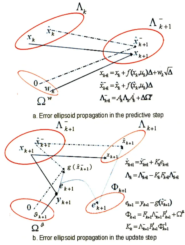
Extended Kalman filter

The above backward recursion system in Theorem 3.1.2 is generally complex to solve as the dimension of states I increases over time. So, out of all information en-capsulated inside Ik, we would like to keep only the useful information. This is where the assumptions of Gaussian distributions in Section 2.5 come into place. In this case, we try to keep conditional means Xk = E[xk lk] and conditional

covari-ances Ak = _{Var[xk Ik] using the Extended Kalman filter (EKF). The EKF has been}

non-linear domains by linearizing the dynamics of systems and measurements. The summary of how the EKF works is described in the following theorem.

-f-=ji~ +f(s2,uk)A

IQ =4M\4

+AU

a. Error ellipsoid propagation in the predictive step

.1

k+l

KkA+,

-Wkc+

4

₁

b. Error ellipsoid propagation in the update step

Figure 3-1: The extended Kalman filter.

0 W

ALn

12,

,

41

+ 4ek~

Aýý 1

Y., +

Ct

k+

Q

6

Theorem 3.2.1. (The extended Kalman filter) Assume that the system together with

its measurement output is described by

Xk+1 = Xk + f(Xk, Uk)A + Wk/, k = 0, 1, ..., N - 1 (3.33)

Yk = g(xk) + ?k, k = 0, 1, ..., N. (3.34)

Assume that a control input Uk at time k is given. The conditional mean Xk+l and

conditional covariance Ak+1 of a system state at time k + 1 after observing a

mea-surement Yk at time k are computed recursively via the following two steps: Predictive step: k+1=

k

+

f(k,

(3.35)

OX

AQw.

F+

_k+1

Information form: Alternatively, we can maintain the information form of the EKF, which stores and updates the inverses of conditional covariances and informa-tion vectors v as:

= (A-+)-1 (3.42)

( k+1 (Ak+1 A )+1, (3.42)

'k+1 = F+j (Qv-1yk+1 + Vk-+1,

(3.44)

A-1 = (Ak+ 1)- 1 + F+1v)-Fk+. (3.45)

The interpretation of the EKF is depicted graphically in Figure 3-1. As we can see, the ellipses represent the contour of equal probability around the means. The dashed lines depict the dynamics of the mean values, while the solid lines represent the actual values of random variables.

The following lemma and Theorem provide another way to update covariance matrices.

Lemma 3.2.1. (Inversion lemma)

(A + BC-1)-1 = (ACC- 1 + BC-1)-1 = C(AC + B)-1

Theorem 3.2.2. If a conditional covariance is factored as Ak = BkC- 1, _{the predictive}

conditional covariance in Eq. 3.37, and the update conditional covariance in Eq. 3.41 can be factored as

Ak+1 - k+ (+) -1, (3.46)

Ak+1 = Bk+lCk+1,

(3.47)

where

* B+, and C4+1 1 are linear functions of B' and Ck

* Bk+1 and Ck+1 are linear functions of 8+ 1 and Ck+1.

Proof. From Ak = B3_{kC-l,using the inversion lemma, we have:}

A+1 = AkA'k + A'l (3.48)

= AkBkCk-'A' + AOw _(3.49)

S((AkBk)

((Ak)-lCk)l+

_(3.50)