HAL Id: hal-00554781
https://hal.archives-ouvertes.fr/hal-00554781
Preprint submitted on 11 Jan 2011HAL is a multi-disciplinary open access archive for the deposit and dissemination of sci-entific research documents, whether they are pub-lished or not. The documents may come from teaching and research institutions in France or
L’archive ouverte pluridisciplinaire HAL, est destinée au dépôt et à la diffusion de documents scientifiques de niveau recherche, publiés ou non, émanant des établissements d’enseignement et de recherche français ou étrangers, des laboratoires
Simulation of Quantum Mechanics Using Reactive
Programming
Frédéric Boussinot
To cite this version:
Frédéric Boussinot. Simulation of Quantum Mechanics Using Reactive Programming. 2011. �hal-00554781�
Simulation of Quantum Mechanics
Using Reactive Programming
∗Fr´
ed´
eric Boussinot
INRIA / INDES
06902 Sophia-Antipolis Cedex, France
Abstract
We implement in a reactive programming framework a simulation of three aspects of quan-tum mechanics: self-interference, state superposition, and entanglement. The simulation basi-cally consists in a cellular automaton embedded in a synchronous environment which defines global discrete instants and broadcast events. The implementation shows how a simulation of fundamental aspects of quantum mechanics can be obtained from the synchronous parallel combination of a small number of elementary components.
Keywords. Computer Science; Parallelism; Reactive Programming; Cellular Automata; Quantum Me-chanics
1
Introduction
The work described here is an exercise in parallel programming inspired by Physics (more precisely, by R. Penrose’s books [9, 10]). Actually, it presents a simulation intended to reflect three rather intriguing aspects of Quantum Mechanics (QM):
1. Self-interference: this is basically Young’s experiment where a particle interferes with itself when passing through two slits.
2. Superposition: the state of a particle is a superposition of several basic states which disappears when a measure occurs.
3. Entanglement: a measure performed on one element of a pair of entangled particles has an instantaneous effect on the other.
The main objective of the simulation is to build global behaviours as parallel compositions of elementary ones. The variant of parallelism used is the synchronous one [6]. The goal is not to exactly model reality (actually, one gets something which is is certainly not a good model of reality as it does not compute over probabilities) but to mimic some aspects of it, linked to QM.
We adopt Penrose’s terminology and call U and R the two basic procedures of QM. The U procedure corresponds to the evolution of a system described by a state |ψi which evolves according to the rule:
i~ d
dt|ψi = H|ψi (1)
This rule is deterministic and linear (any linear combination of solutions is also a solution). The R procedure corresponds to a change of state of |ψi of the form:
|ψi =X
a
|aiha|ψi → |ai (2)
The superposition state |ψi becomes the basic state |ai; the probability of this change is |ha|ψi|2.
The rule R is nondeterministic and probabilistic.
We make the assumption of a discrete world built over a cellular automaton (CA) [11], im-plementing the U procedure. We do not model fields, which are non-discrete objects, but CA’s which are discrete ones. Actually, in CA’s, both space and time are discrete. The rate at which a CA is simulated is the limit speed1
of the system. CA’s are embedded in a synchronous world which is actually the one of the simulation. There are thus global instants during which actions are considered as simultaneous. The basic hypothesis is that the U procedure is deterministic and local (thus, not instantaneous, as it can take several instants for a change to propagate in space). On the opposite, the R procedure is nondeterministic, global, and instantaneous (in a sense to be made precise later). The main basic notions are: synchronous parallelism, determinism of U and nondeterminism of R, discrete space (CA) and discrete time (synchrony hypothesis).
In the simulation, a (virtual) particle at instant t is represented by a set of cells living at instant t. Each cell is in a basic state of the particle, and the particle global state is the superposition of all the basic states of the associated cells. Basic states are identified by specific colors and cells are drawn according to the basic state they hold. When superposition disappears, after execution of procedure R, one cell is chosen randomly and the created (real) particle falls in the basic state of the chosen cell (the particle then receives the color of the cell). Thus, the probability for a particle to fall in a given basic state |ai depends on the number of cells holding this state: the more there are cells holding |ai, the more the probability to choose |ai is high.
A measure is implemented by the emission of a broadcast event that is instantaneously received by all the cells implementing the measured object. This is basically the R procedure. In reaction
1
to R, one cell is nondeterministically chosen and the real particle is produced from that cell (with its basic state).
A particle is virtual when it is implemented by the CA. It turns to real after application of the R procedure. A real particle is animated by the synchronous simulation; it is a data structure with coordinates and speed, animated by several elementary parallel behaviours (for example, an inertia behaviour, which at each instant sets the coordinates according to the speed, and a bouncing behaviour which makes the particle bounce on the simulation borders2
. The simulation basically shows the following aspects:
1. Self-interference is illustrated by Young’s experiment where a particle is emitted against a wall with two slits. The particle passes through both slits, which produces interferences. The simulation shows the production of interferences, and their disappearance when one slit is obstructed.
2. The simulation shows the production of a real particle when a detector reacts to the presence of a living cell; in this case, the R procedure entails the reduction to a basic state.
3. Pairs of entangled particles are considered. The measure of one element of the pair triggers the R procedure for it, which produces a real particle. The measure also triggers the R procedure for the second particle. Moreover, it forces the choice of the basic state of the real particle produced from the second virtual particle.
Section 2 describes the simulation. Section 3 describes the implementation and gives the most important pieces of code. Some related work is described in Section 4. Finally, Section 5 concludes the text.
2
The Simulation
We consider particles whose states are superpositions of basic states which are integers modulo k (ZZ/kZZ); in the sequel, k is called the base, and we arbitrarily set it to 6. Thus, there are 6 distinct basic states:
#|ai = 6 (3)
Each basic state is assigned a distinct color. A superposition is a (finite) sequence of basic states. Figure 1 shows the representation of a superposition.
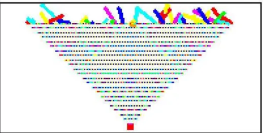
The emission of a particle by a source is represented in Figure 2. The source is at the bottom of the figure (big red square). The simulation is enclosed by a wall (black cells) that forces the particle to stay inside the delimited area. The particle is emitted in direction of the top. Its superposition states are shown, as time passes. The left part of the figure shows one instant, before the particle
2
Figure 1: Superposition State
reaches the wall. In the right part are collected all the traces of the particle until it reaches the wall; the image obtained is typical of a cellular automaton (this point will be discussed later).
Figure 2: Particle Emission
Detectors are special cells that react when a superposition state reaches them. Figure 3 shows a detector (big orange square) reacting to a superposition state reaching it. A particle is created on the right side (with a basic state corresponding to the pink color).
Figure 3: Detection
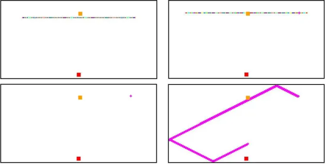
Figure 4 shows a sequence of events corresponding to the detection of a particle. The top-left image shows the situation just before detection. The particle is in a superposition state. The top-right image shows the detection of the particle. The R procedure is performed and a basic state is chosen. It is actually the state of a cell colored in pink, on the right side of the superposition state. The bottom-left image shows the situation just after R: the superposition has disappeared and a new particle is created with the pink basic state. The bottom-right image shows the trajectory of the particle, bouncing on the wall, after some instants.
Figure 4: Detection Sequence
Figure 5 shows the production of a flux of identical particles (i.e. initially in the same basic state) which are detected in turn. Traces of the produced particles are shown on the part of the image situated over the detector.
2.1 Young’s Experiment
A new wall is introduced in Figure 6 which separates the simulation in two parts. In the left image, two slits are present; in the right image, the right slit is obstructed. This basically corresponds to Young’s experiment. In the right image, the structure under the separation wall is reproduced over the separation wall. In the left part, the two structures produced from the two slits interfere when they overlap.
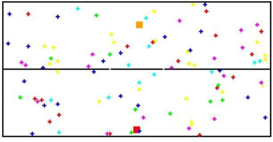
We now consider the detection of particles in Young’s experiment. Figure 7 shows the situation after detection of 100 particles (in presence of 2 slits).
Once the number of slits is fixed, all particles reach the detector in the same superposition of basic states (because U is deterministic and local). When the R procedure is executed, a cell is randomly chosen from the superposition and the particle gets the cell basic state. The probability for a particle to fall on the basic state |ai only depends on the percentage of cells with state |ai appearing in the superposition. The superposition state thus directly codes the probabilities associated with the basic states. The probability of a basic state |ai in a superposition S is:
Figure 5: Multiple Detections
Figure 6: Young’s Experiment
P rob(|ai, S) = #a ∈ S
#S (4)
These probabilities depend on the number of slits, on the localisation of the detector and on the localisation of the slits. Here is for example a typical result (with 1000 particles):
basic state 0 1 2 3 4 5
1 slit 0.327 0.023 0.281 0.153 0.017 0.199 2 slits 0.226 0.039 0.298 0.171 0.116 0.150
Figure 7: Young’s Experiment - 2
to fall in state 0 with 1 slit, while it has probability 0.226 to fall in the same state with 2 slits.
2.2 Entanglement
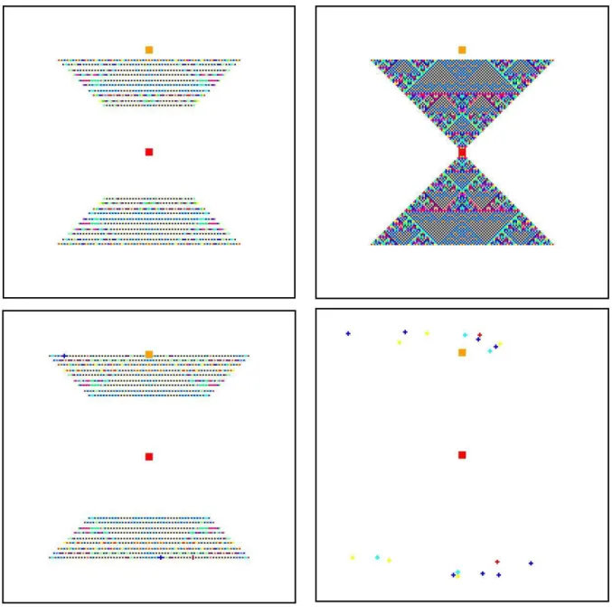
We now consider pairs of entangled particles emitted by the same source. Each pair is composed of a particle emitted in the top direction and an entangled particle emitted in the bottom direction. Entanglement basically means two things: first, the two particles share the same R procedure; second, the choices of basic states implied by R are not independent (to simplify, we consider that the two particles always choose the same basic state). An example of 10 emissions of pairs of entangled particles is shown in Figure 8:
• The top-left image shows the situation where all the pairs have been emitted by the source but none has yet been detected. Two beams of particles are present, one directed to the top and one to the bottom.
• The same situation is shown on the top-right image, but traces of the particles are kept visible (remanent images).
• The bottom-left image shows the detection of a particle (blue) by the detector (big orange square). The entangled particle (also blue) appears at the bottom of the image.
• In the bottom-right image, all 10 particles have been detected. The 10 corresponding entan-gled particles are present at the bottom of the image.
3
Implementation
The simulation is implemented in the FunLoft programming language [4, 1]. CA’s and particles have been previously implemented in several contexts of reactive programming (e.g. in the two research papers [2] and [3]; the simulation described here uses elements of both papers).
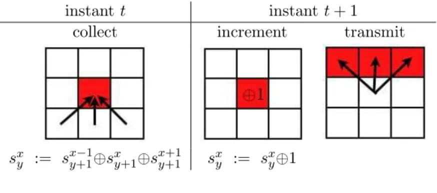
Basically, we consider a cellular automaton embedded in a reactive simulation. The reactive simulation runs reactive threads (simply called threads in the sequel) in a cooperative way, and defines global instants shared by all the threads. According to the presence of instants, threads can synchronise and communicate with broadcast events. Instants and evolution steps of the cellular automaton are identified. Each cell of the underlying cellular automaton is implemented by a thread; moreover, particles created in response to measures are also implemented with threads. The cell rule is described in Figure 9 (for the top direction). A cell living at instant t (in red) collects the activations of the 3 cells under it and increments its state by the collected values (⊕ denotes addition modulo 6); then, at instant t + 1, the cell increments its state by 1, and transmits it to the 3 cells above it.
instant t instant t + 1
collect increment transmit
sx y := s x−1 y+1⊕s x y+1⊕s x+1 y+1 s x y := s x y⊕1
Figure 9: Cell Rule
Cells that are living at instant t form the superposition state at instant t. When a measure occurs, an event is broadcast to all the living cells, which stops their transmission step. Moreover, one of the living cells is randomly chosen and a particle is created from it.
The simulation is approximatively made of 1400 lines of code; in this section, we only give the main parts of the code. The section is structured as follows: the data structure of cells is described in Section 3.1. Section 3.2 describes the activation of cells (U procedure). The cell behaviour combining both U and R is described in 3.3. Section 3.4 describes the R procedure. The source of single particles is described in 3.5 and the source of entangled particles is described in 3.6.
3.1 Cell Data Structure
type cell_t = cell of x: int
* y: int
* kind: cell_kind_t ref * living: bool ref * basic_state: int ref
* trigger: (activation_t) event_t * R: (unit) event_t ref
* signal: (int) event_t ref * chosen: int ref ref * chosen_state: int ref ref
In this definition:
• x and y are the cell coordinates;
• kind is the cell kind, that is, the direction of the particle (UP or DOWN), or BRICK for cells belonging to a wall;
• living holds true when the cell is living and false when it is dead;
• basic state holds the basic state associated with the cell;
• trigger holds the event used by neighbours to activate the cell; the event has a value of type activation twhich describes the characteristics of the triggering neighbour (see 3.2);
• R holds the event used by the R procedure;
• signal holds the event used to signal the basic state of the cell;
• chosen holds the chosen cell, when chosen, and -1 otherwise.
• chosen state holds the chosen state, when chosen, and -1 otherwise.
Note that chosen and chosen state are doubly referenced because they can be both communi-cated and changed (as example, chosen state is needed for entanglement, in order to be be shared among the entangled particles).
Basic states are integers modulo base; we define add state that adds an integer to a cell basic state, and increm state that increments a cell basic state:
let add_state (c,z) =
let a = cell.basic_state (c) in a := (!a + z) mod base
3.2 Neighbours
Cells trigger their neighbours by giving them an activation record which is a data-structure defined by:
type activation_t = activation of * kind: cell_kind_t
* basic_state: int * R: (unit) event_t * signal: (int) event_t * chosen: int ref * chosen_state: int ref
In order to trigger a neighbour, a cell generates the trigger event of the neighbour with an activation record describing itself (nothing is done if the neighbour is a brick):
let awake_neighbour (c,ix,iy) =
let neighbour = !cell_array [cell.x (c) + ix,cell.y (c) + iy] in let state = !cell.basic_state (c) in
let kind = !cell.kind (c) in let r = !cell.R (c) in
let signal = !cell.signal (c) in let chosen = !cell.chosen (c) in
let chosen_state = !cell.chosen_state (c) in if !cell.kind (neighbour) <> BRICK then
generate cell.trigger (neighbour) with
activation (kind,state,r,signal,chosen,chosen_state) end
Here is the part corresponding to the UP direction of the function that triggers the neighbourhood of a cell: let awake_neighbourhood (c) = let k = !cell.kind (c) in if k = UP then begin awake_neighbour (c,-1,-1); awake_neighbour (c,0,-1); awake_neighbour (c,1,-1); end else ...
The cells triggered are the cell c1 situated immediately above c, and the two cells at the right and at the left of c1.
The other directions are processed in a similar way that we do not describe here for the sake of conciseness.
When triggered by a neighbour, a cell combines the associated activation record with itself. We choose a very simple combination scheme: the state of the triggering cell is added to the state of the activated cell. The function combine is defined by:
let combine (c,activ) = begin
cell.kind (c) := activation.kind (activ); add_state (c,activation.basic_state (activ)); cell.R (c) := activation.R (activ);
cell.signal (c) := activation.signal (activ); cell.chosen (c) := activation.chosen (activ);
cell.chosen_state (c) := activation.chosen_state (activ); end
3.3 Cell Behaviour
The U procedure basically implements the behaviour described in Figure 9: each cell living at instant t collects the activations from the cells below it, adding their states to its current state; then, at instant t + 1, the cell increments its state and activates the three cells above it. A cell thus transmits to the cells above the collection of the states of the cells below it, after having incremented its own state. More precisely, the behaviour of a cell is the following (we do not consider here the case of bricks)3
:
let module cell_behavior (c) = loop
begin // step1
if !cell.living (c) then awake_neighbourhood (c) else begin await cell.trigger (c); cell.living (c) := true; end; // step2
for_all_values cell.trigger (c) with a -> combine (c,a); increm_state (c);
display (c); // step3
let r = ref Nil_list in begin
3
get_all_values !cell.R (c) in r; if length (!r) <> 0 then // R called
let done = event in begin
thread reduce (c,done); await done; end else awake_neighbourhood (c) end; // step4 cell_reset (c); end
This cyclic behaviour (loop) is composed of the following steps:
step1: if the cell is living, then the neighbours are triggered (awake neighborhood). Otherwise, the cell awaits to be triggered (await).
step2: the cell collects all the values generated by its neighbours (for all values) and combines them (combine). Then, the cell increments its state (increm state) and displays itself on screen (display).
step3: the possibility of reduction with the R procedure is considered. All the values associated with the R event are collected (get all values). If the collected list is not empty, then an instance of the reduce module is launched and its termination is awaited using the new event done. Otherwise, the neighbours are triggered.
step4: the cell is reset (cell reset); this function basically resets the basic state, records the cell as dead, and erases it on screen.
3.4 Reduce Procedure
Let us consider the module that chooses a basic state from a superposition. First, it awaits the signal event which is generated by all the cells involved in the superposition when the R procedure is executed. Each cells gives its identity (under the form of a linear combination of its coordinates) together with the signal. Then, all the identities are collected and one is chosen nondeterministically using the variable chosen (initially, chosen equals -1; when the first choice occurs, chosen is set to the identity of the chosen cell, returned by the function choose):
let module choose_in_superposition (c) = let signal = !cell.signal (c) in let chosen = !cell.chosen (c) in let collect = ref Nil_list in
begin
await signal;
get_all_values signal in collect; if !chosen = -1 then
chosen := choose (!collect) end
end
The module that implements the R procedure first launches a thread to choose a basic state. At the next instant (to let the launched thread start execution), it signals itself. Then, after two instants, if it is chosen then it sets the chosen state (set chosen state) and launches a particle bearing the color of the chosen state (particle behavior). The code is:
let set_chosen_state (c) =
if !!cell.chosen_state (c) = -1 then
!cell.chosen_state (c) := !cell.basic_state (c) end
let module reduce (c,done) = let x = cell.x (c) in let y = cell.y (c) in let me = linear (x,y) in
begin
thread choose_in_superposition (c); cooperate;
generate !cell.signal (c) with me; cooperate; cooperate; if !!cell.chosen (c) = me then begin set_chosen_state (c); let fx = int2float (x) in let fy = int2float (y) in let dir = cell.kind (c) in
let state = !!cell.chosen_state (c) in
thread particle_behavior (fx,fy,cell_color (state),dir) end
end;
generate done end
3.5 Source
The firing function generates the triggering event of a cell, with an activation made of a new signal and a new reference holder for chosen:
let fire (c,a,dir,e,s) =
generate cell.trigger (c) with activation (a,e,dir,event,ref -1,s)
A (standard) source cyclically fires a cell when receiving the event go. Each fired particle has a new event R and a new state holder for chosen state. All particles are initially in the same basic state.
let module source_r (x,y,s,dir,go) = let c = !cell_array [x,y] in
loop begin
await go;
fire (in_dir (c,dir),s,dir,event,ref -1); cooperate;
end
3.6 Entanglement
A source of entangled particles emits two particles in opposite directions, but sharing the same R event and the same state holder. Thus, when one of the entangled particles is detected, it is exactly as if the other was also detected, at the same instant; moreover, the choice of the basic state made for the detected particle is instantaneously transmitted to the other particle. The code of the source producing entangled particles in opposite directions is:
let module dual_source_r (x,y,s,dir,inv,go) = let c = !cell_array [x,y] in
loop
let r = event in // shared R
let sh = ref -1 in // shared state holder begin
await go;
fire (in_dir (c,dir),s,dir,r,sh); fire (in_dir (c,inv),s,inv,r,sh); cooperate;
end
Note that the state holder is a “shared reference” which can be assigned and read by entangled particles. These shared references are different from “hidden variables” that would be set at creation of the entangled pair, but that would not be readable (“hidden”) by any measure. In the simulation, there is actually an instantaneous (i.e. during the same instant) communication that occurs between the two entangled particles when R occurs (and not before that moment).
4
Related Work
Simulation of physics with computers has been initiated by R. Feynman in [5]. His paper ends with:
“And I’m not happy with all the analyses that go with just the classical theory, because nature isn’t classical, dammit, and if you want to make a simulation of nature, you’d better make it quantum mechanical, and by golly it’s a wonderful problem, because it doesn’t look so easy.” Feynman directly spoke to computer scientists, saying: “... what I’m trying to do is to get you people who think about
computer-simulation possibilities to pay a great deal of attention to this, to digest as well as possible the real answers of quantum mechanics, and see if you can’t invent a different point of view than the physicists have had to invent to describe this.” The initial motivation for the simulation proposed here was to understand quantum mechanics. And to understand something, what’s could be better than to implement it?
In [7], B. Hayes discusses the issue of writing programs to implement a physically plausible universe. He considers the use of cellular automata and notes that “The global clock is surely
an uninvited guest in the world of cellular automata. Having taken pain to create a purely local computational physics, we then introduce a signal that must be broadcast to every point in the universe in every moment of time. What could be less local than that?”. This remark is totally relevant for the simulation presented here, but we don’t see any alternative to model instantaneous aspects of QM (as a matter of fact, we see instantaneity as the strangest aspect of QM).
In [12] J. A. Wheeler compares nature and computers. He says “Time is not a primary category
in the description of nature. It is secondary, approximate, and derived.” Our simulation actually introduces two levels of time. The first level is the level of instants which is global to both CA cells and (real) animated particles; at that level, events are completely ordered and causality is totally defined. The second level concerns the events occurring during the same instant; they are not totally ordered and the causality is a “loose” one in which the notions of “before” and “after” are not totally strict and depend on the implementation.
To consider the universe as a computing machine (Digital Physics) is an idea which may be found for example in K. Zuse’s work, where the computer is a cellular automaton. S. Lloys [8] considers a quantum computer instead. Here, we describe a cellular automaton embedded in a reactive environment, naturally introducing global instants and broadcast events, and we do not consider any aspect of quantum computing.
5
Conclusion
We have implemented a simulation with the following characteristics:
• The simulation is composed of a cellular automaton embedded in a reactive environment providing global instants and broadcast events.
the cellular automaton is implemented by a thread. After detection, each particle is animated by several threads of the reactive environment.
• The cells living at instant t code the superposition state of the particle at instant t. Before detection, the evolution of the particle is defined by the cellular automaton rule (U procedure).
• Detection of a particle generates a broadcast event, instantaneously received by all the cor-responding living cells of the cellular automaton.
• After detection, living cells are instantaneously reset, and a particle animated by the reactive environment is created. The state of the created particle is randomly chosen among the basic states composing the superposition (R procedure). This is the only source of nondeterminism in the simulation.
• Entanglement of particles basically means that they share the same procedure R. The shared event corresponding to R is instantaneously broadcast to all entangled particles by the reac-tive environment.
There are at least two regards in which the simulation could certainly be improved:
• In the current simulation, superposition states are segments; they could be replaced by circular shapes centered on the source. Hexagonal CA’s could be useful for that purpose.
• One may wonder how to introduce gravity, for particles that have a mass. With real particles, this is not a problem: gravity can be naturally implemented as a field. But it is not clear how to introduce gravity when the particle is virtual (the cell rule of the cellular automaton should implement it).
Acknowledgments. Many thanks to Guillaume Boussinot for his remarks, criticisms, and sug-gestions.
References
[1] FunLoft. http://www-sop.inria.fr/indes/rp/FunLoft.
[2] F. Boussinot. Reactive Programming of Cellular Automata, 2006. http://hal.inria.fr/inria-00071405.
[3] F. Boussinot. A Benchmark for Multicore Machines, 2007. http://hal.inria.fr/inria-00174843.
[4] F. Boussinot. Safe Reactive Programming. The FunLoft Language. Lambert Academic Pub., 2010.
[5] R. P. Feynman. Simulating Physics with Computers. International Journal of Theoretical
Physics, 21(6/7), 1982.
[6] N. Halbwachs. Synchronous Programming of Reactive Systems. Kluwer Academic Pub., 1993.
[7] B. Hayes. Debugging the Universe. International Journal of Theoretical Physics, 42(2), 2003.
[8] S. Lloyds. Programming the Universe: A Quantum Computer Scientist Takes On the Cosmos. Knopf, 2006.
[9] R. Penrose. The Emperor’s New Mind. Concerning computers, minds, and the laws of physics. Oxford University Press, 1989.
[10] R. Penrose. The Road to Reality. A Complete Guide to the Laws of the Universe. Jonathan Cape, 2004.
[11] T. Toffoli and N. Margolus. Cellular Automata Machines. A new Environment for Modeling. The MIT Press, 1987.
[12] J. A. Wheeler. The Computer and the Universe. International Journal of Theoretical Physics, 21(6/7), 1982.