HAL Id: hal-01526643
https://hal.archives-ouvertes.fr/hal-01526643
Submitted on 18 Dec 2019
HAL is a multi-disciplinary open access
archive for the deposit and dissemination of
sci-entific research documents, whether they are
pub-lished or not. The documents may come from
teaching and research institutions in France or
abroad, or from public or private research centers.
L’archive ouverte pluridisciplinaire HAL, est
destinée au dépôt et à la diffusion de documents
scientifiques de niveau recherche, publiés ou non,
émanant des établissements d’enseignement et de
recherche français ou étrangers, des laboratoires
publics ou privés.
Resolution and reconciliation of non-binary gene trees
with transfers, duplications and losses
Edwin Jacox, Mathias Weller, Eric Tannier, Celine Scornavacca
To cite this version:
Edwin Jacox, Mathias Weller, Eric Tannier, Celine Scornavacca. Resolution and reconciliation of
non-binary gene trees with transfers, duplications and losses. Bioinformatics, Oxford University Press
(OUP), 2017, 33 (7), pp.980-987. �10.1093/bioinformatics/btw778�. �hal-01526643�
Resolution
and reconciliation of non-binary gene
trees
with transfers, duplications and losses
Edwin
Jacox
1
,
Mathias Weller
2,3
,
Eric Tannier
4
and
Celine Scornavacca
1,2,⇤
1
ISE-M, Université Montpellier, CNRS, IRD, EPHE, Montpellier, France
2Institut de Biologie Computationnelle (IBC), Montpellier,France
3LIRMM, Université Montpellier, CNRS, Montpellier, France
4INRIA Rhône-Alpes, LBBE, Université Lyon 1, Lyon, France
⇤To whom correspondence should be addressed.
Abstract
Motivation:
Gene trees reconstructed from sequence alignments contain poorly supported branches when
the phylogenetic signal in the sequences is insufficient to determine them all. When a species tree is
available, the signal of gains and losses of genes can be used to correctly resolve the unsupported parts of
the gene history. However finding a most parsimonious binary resolution of a non binary tree obtained by
contracting the unsupported branches is NP-hard if transfer events are considered as possible gene scale
events, in addition to gene origination, duplication and loss.
Results:
We propose an exact, parameterized algorithm to solve this problem in single-exponential time,
where the parameter is the number of connected branches of the gene tree that show low support from the
sequence alignment or, equivalently, the maximum number of children of any node of the gene tree once
the low-support branches have been collapsed. This improves on the best known algorithm by an
exponential factor. We propose a way to choose among optimal solutions based on the available
information. We show the usability of this principle on several simulated and biological data sets. The
results are comparable in quality to several other tested methods having similar goals, but our approach
provides a lower running time and a guarantee that the produced solution is optimal.
Availability:
Our algorithm has been integrated into the ecceTERA phylogeny package, available at
http://mbb.univ-montp2.fr/MBB/download_sources/16__ecceTERA
and which can be run
online at http://mbb.univ-montp2.fr/MBB/subsection/softExec.php?soft=eccetera.
Contact:
celine.scornavacca@umontpellier.fr
1 Introduction
Constructing good gene trees is both crucial and very challenging for molecular evolutionary studies. The most common way to proceed is to compute a multiple alignment of nucleotide or protein sequences from a gene family, and search for an evolutionary tree that is most likely to produce this alignment (under some evolutionary model). Additionally, it is strongly advised to compute statistical supports on the branches of the output tree, as this tells whether they are inferred from the signal of mutations contained in the alignment or are chosen at random in the absence of signal (Felsenstein, 2004). Commonly, it is very rare that the gene sequences contain enough mutations, but not too many, to support all the branches of a gene phylogeny (Mossel and Steel, 2005).
In consequence, it is very rare that a maximum-likelihood tree computed from a multiple alignment reflects the true history of the genes.
A way to approach this true history is to use the information contained in a species tree to correct the branches of the gene tree that are not supported by the alignment. Understanding a gene tree, given its species tree, requires the introduction of gene scale events, as the birth of the gene, its death, its replication and diversification by speciation, duplication, and horizontal gene transfer (Szöll˝osi et al., 2015). Such a complete history is called a reconciliation and, if costs are assigned to each gene scale event, it has a total cost. Binary gene trees reconstructed with the additional information of this reconciliation cost show a higher quality, according to all tests on methods that are able to perform such a construction: MowgliNNI (Nguyen et al., 2013), ALE (Szöll˝osi et al., 2013), TERA (Scornavacca et al., 2015), TreeFix-DTL (Bansal et al., 2014) and JPrIME-DLTRS (Sjöstrand et al., 2014) (we enumerate only the methods allowing
horizontal gene transfers). However, these methods generally require intensive computation time.
Here, we provide an algorithm that, given a species tree S and a gene tree G with supports on its branches, computes a modified gene tree G0
such that all well-supported branches of G are in G0and no other gene
tree modified in such a way has a lower reconciliation cost than G0. “Well
supported” is defined by a threshold chosen by the user, or by an adaptive method which sets this support according to the algorithm complexity. This problem reduces to the reconciliation of non-binary gene trees with binary species trees. Although optimal and practical methods are known in the absence of gene transfers (Noutahi et al., 2016), this problem has been shown to be NP-hard (Kordi and Bansal, 2015) with gene transfers. Letting k be the maximum number of children of any node of the gene tree after collapsing branches of low support, the problem can be solved in 2k· kk· (|S| + |G|)O(1)time (Kordi and Bansal, 2016). We employ
amalgamation principles (David and Alm, 2011; Szöll˝osi et al., 2013; Scornavacca et al., 2015) to provide an algorithm with a time complexity of (3k 2k+1)·(|S|+|G|)O(1), which gives access to a wider range of data.
This, however, comes at the price of using ⇥(2k)space while the algorithm
of Kordi and Bansal (2016) runs in polynomial space. We provide an implementation of our algorithm and we propose a way to choose among all optimal solutions according to the supports of the branches of the input tree. We show on both simulated and real data sets that our method produces gene trees whose quality is similar to those constructed by competitive methods, often in a smaller amount of time.
The novelties of this method compared to the previous ones are: (1) a lower running time, allowing it to run on larger datasets; (2) guaranteed optimal solutions; and (3) a simpler input – the input data consists of a gene tree with supports and a species tree, without the need to supply a gene alignment or a sample of gene trees that other methods rely on. Moreover, our method is integrated into the user-friendly ecceTERA package so that anyone having a gene tree with supports – output by standard ML software such as PhyML or RAxML – and a species tree (with or without dates), can quickly obtain a better-quality gene tree, or even correct a whole database in reasonable time.
2 An FPT algorithm for reconciling gene trees
with polytomies
2.1 Reconciliation of binary gene trees
For our purposes, a rooted phylogenetic tree T = (V (T ), E(T ), r(T )) is an oriented tree, where V (T ) is the set of nodes, E(T ) is the set of arcs, all oriented away from r(T ), the root. For an arc (x, y) of T , we call x the parent of y, and y a child of x. The number of children of x, denoted by kx, is called the out-degree of x. If a path from the root to y contains
x, then x is an ancestor of y and y is a descendant of x. This defines a partial order denoted by y T x, and y <Txif x 6= y. The subtree of
Tthat is rooted at a node u of T (denoted by Tu) is the result of deleting
all nodes v with v ⇥T ufrom T . Nodes with no children are leaves, all
others are internal nodes. The set of leaves of a tree T is denoted by L(T ). The leaves of T are bijectively labeled by a set L(T ) of labels. A tree is binary if kx= 2for all internal nodes x. A tree T is dated if a total order
✓on internal nodes that extends Tis given. Each internal node then
implies a date between 1 and |V (T )| |L(T )| (the root) and all the leaves are assumed to have date 0. The dated subdivision T0of a dated tree T
is obtained by replacing each arc (x, y) by a path containing d additional nodes, where d+1 is the difference between the date of x and the date of y. A reconciliation involves two rooted phylogenetic trees, a gene tree G and a species tree S, both binary. Their relation is set by a function s : L(G) ! L(S), which means that each extant gene belongs to an extant species. Note that s does not have to be injective (several genes
of G can belong to the same species) or surjective (some species may not contain any gene of G). A reconciliation ↵ of G in S is a mapping of each internal node u of G to a sequence(↵(u)1, ↵(u)2, . . .) of nodes of S if S is undated or nodes of the dated subdivision S0of S
if S is dated. Herein, for each i 1, we have ↵(u)i+1 T ↵(u)i
and ↵(u)i satisfies the constraints of any one of the possible events
among duplication (D), transfer (T), loss (L), or speciation (S) – see the appendix in the supplementary material for more details. This ensures that a coherent gene history can be extracted from ↵. Given costs for individual D, T and L events (it is usually assumed that speciation does not incur cost), denoted respectively , ⌧ and , a reconciliation ↵ is assigned the cost c(↵) := d + t⌧ + l , where d, t and l denote the respective numbers of events of type D, T and L implied by ↵. We denote by R(G, S) the set of all possible reconciliations of G in S and define cDTL(G, S) := min↵2R(G,S)c(↵), that is, the minimum cost over all
possible reconciliations of G in S. We call cDTL(G, S)the cost of G with respect to a species tree S. A reconciliation ↵ achieving this cost is called most parsimonious reconciliation (MPR).
Problem 1. Most Parsimonious Reconciliation
Instance: a (dated) binary species tree S, a binary gene tree G, costs , ⌧, for respective D, T, L events
Output: a reconciliation of G in S of minimal cost
This problem can be solved in O(|S|2· |G|) time (Doyon et al., 2010)
for dated trees, and O(|S| · |G|) time for undated ones (Bansal et al., 2012). In the following, we turn our attention to non-binary gene trees and we consider the species tree as dated. Nevertheless, every result is also valid for the undated case with better complexity, see Section 3.3.
2.2 Resolution of non-binary gene trees
If a node in a tree T has more than two children, we call this node a polytomy. Note that a node a of T partitions L(T ) into two sets, the descendants of a and all others. Given a gene tree G with at least one polytomy, a binary tree G0is called a binary resolution of G if G can be
obtained from G0by contracting edges. We denote by BR(G) the set of
all binary resolutions of G.
Problem 2. Polytomy Solver under the DTL framework
Instance: a dated binary species tree S, a gene tree G, costs , ⌧, respectively for D, T, L events
Output: a binary resolution G0of G minimizing cDTL(G0, S)
This problem – introduced by Chang and Eulenstein (2006) – is known to be NP-hard (Kordi and Bansal, 2015), and can be solved in time O(|G|+|S|) for ⌧ = 1 (Zheng and Zhang, 2014b).
A brute-force approach would need to generate all binary resolutions. There are (2n 3)!!⇡p2(2
e(n 1))n 1different rooted binary trees
on n leaves, which gives | BR(G)| ⇠ Qu2V (G)\L(G)
p 2(2e(ku
1))ku 1different binary resolutions of G. This yields an algorithm with
time complexity O(|S|2· |G| · | BR(G)|). Using the following result, we
can improve on the brute-force approach.
Theorem 2.1. Let S be a species tree, let G be a gene tree, and let u be a polytomy in G.Let G02 BR(G) and let ↵ 2 R(G0, S)such that
↵is an MPR between S and G0and no MPR between S and any other
binary tree in BR(G) is strictly cheaper than ↵.Let G⇤
u2 BR(Gu)and
let 2 R(G⇤u, S)such that (u)1 = ↵(u)1. Then, c(↵u) c( ),
where ↵uis the restriction of ↵ to G0u.Less formally, a binary resolution of G allowing a globally optimal reconciliation ↵ is also locally optimal for each subtree rooted at a polytomy u (provided that u is mapped to the same species v).
This implies that an MPR ↵ on the whole tree G always yields an MPR on a subtree Gu (where the first node in the mapping of u is
constrained to be the same as in ↵); so we can progressively reconstruct a global solution by amalgamating MPRs on subtrees.We do not give a proof of Theorem 2.1 here because it will be a consequence of our main Theorem 2.2. Nevertheless, we note here that the dynamic programming algorithm by Doyon et al. (2010) with the help of Theorem 2.1 permits us to solve Problem 2 with a lower complexity: Whenever we encounter a polytomy u in its bottom-up approach, we store, for each v 2 V (S), the minimum cost of a reconciliation associating u with v over all binary resolutions of Gu.
Observation 2.1. A solution for Problem 2 can be found by solving polytomies one by one in a bottom-up approach, with a time complexity of O(|S|2· |G| · (2
e(k 1))k 1), where k is the maximum number of
children of any node in G.
Note that this has been independently observed by Kordi and Bansal (2016), who presented an algorithm having the same asymptotic time complexity as the approach described in Observation 2.1.
While Observation 2.1 already implies that Problem 2 is fixed-parameter tractable1 (FPT) with respect to the maximum out-degree in
G, it remains interesting to search for a single-exponential-time algorithm that could process larger gene trees and even genome-wide data. The idea for such an algorithm comes from the amalgamation principle.
2.3 Amalgamation of gene trees
A node u of a binary tree T is said to generate the clade C(u) = L(Tu).
If u has distinct children ur and ul, we also say that u generates the
tripartition (C(u), {C(ul), C(ur)}), otherwise, u generates the trivial
tripartition (C(u), {?, ?}). Herein, we call C(u) the domain of the tripartition. A binary tree T generates a set of clades and tripartitions, respectively denoted C(T ) and ⇧(T ), which are the clades and tripartitions generated by its nodes.
More generally, for a set of labels L, a clade is a subset of L and a tripartition is a tuple (C, {Cr, Cl}) such that the clades Cr, Clpartition
the clade C. Let ⇧ be a set of tripartitions on L. We denote the set of clades present in ⇧ by C(⇧). Further, ⇧ is said to be complete if it contains L as the domain of some tripartition, and for each tripartition (A, {B, C}) either B = C = ? or ⇧ contains tripartitions with B and C as respective domains. It is easy to see that the set of tripartitions generated by a binary tree is always complete, and conversely, for any complete set of tripartitions ⇧on L, there is at least one binary tree G with L(G) = L, which generates a subset of ⇧. The amalgamation problem is to generate one minimizing the reconciliation cost with respect to a species tree:
Problem 3. Amalgamation under the DTL framework
Input: a complete set of tripartitions ⇧ on a set of labels L, a dated binary species tree S, a labeling function s : L ! L(S) and costs , ⌧,
respectively for D, T, L events
Output: a binary gene tree G minimizing cDTL(G, S)over all binary
gene trees G0 with L(G0) = Land such that the set of tripartitions
generated by G0is a subset of ⇧
This problem can be solved in O(|S|2· |⇧|) time (Scornavacca et al.,
2015). Given a non-binary tree G, we can generate a complete set of tripartitions containing all tripartitions of any binary resolution of G as follows: for each node u of G with child set {u1, . . . , ut}, and for each
I ✓ {u1, . . . , ut}, u generates a tripartition (A, {B, C}) such that 1 An algorithm is FPT with respect to p if its running time is f(p)·poly(n)
where f is some function that only depends on p and n is the size of the instance.
B[ C = A ✓ Si2IC(ui)and none of B or C overlap any C(ui)
(overlapping means containing some elements but not all). The union of all these tripartitions is the set of tripartitions of G, noted ⇧(G) as in the binary case.Now, if the set ⇧ in Problem 3 is set to ⇧(G) and the labelling function s associates the genes in G to the correct species in S, then Problems 2 and 3 are equivalent: indeed, it is easy to see that any binary resolution G0of G is such that the set of tripartitions generated by
G0is a subset of ⇧(G), and that the converse holds too.Thus, theknown
dynamic programming algorithm solving Problem 3 (Scornavacca et al., 2015)yields a novel algorithm for the resolution of polytomies.
Theorem 2.2. Let G be a non-binary gene tree. An amalgamation solution on ⇧(G) is an optimal binary resolution of G.
The complexity of this algorithm is O(|S|2· |⇧(G)|). We can bound
the size of ⇧(G) using the following statement.
Lemma 2.3. For any gene tree G, |⇧(G)| = O(|G| · (3k 2k+1)),
where k is the maximum out-degree of any node in G.
Proof. Let u be a node of G, and u1, . . . , utits children. Recall that,
for each I ✓ {u1, . . . , ut}, u generates a tripartition (A, {B, C}) such
that B [ C = A ✓Si2IC(ui)and none of B or C overlap any C(ui).
Any tripartition (A, {B, C}) generated by u is isomorphic to a partition of {C(u1), . . . , C(ut)} into three sets, B, C, andSiC(ui)\ A with
B6= ? and C 6= ?. There are 3tpartitions of t elements into three sets,
with 2·2tof them having B = ? or C = ?. If the (unique) partition with
B = C =? is not counted twice, we get 3t 2t+1+ 1such partitions.
Finally, we can remove half of the remaining partitions by the symmetry of B and C and arrive at a count of1/2(3t 2t+1+ 1). Thus, there are 1/2(3t 2t+1+ 1)such partitions and, hence, this is also an upper bound
on the number of tripartitions generated by u. Summing over all vertices of G, the total number of tripartitions generated by G is then bounded by |G| ·1/2(3k 2k+1+ 1)where k is the maximum out-degree in G.
This leads to the main theoretical result of the paper
Proposition 2.4. For any gene tree G, Problem 2 can be solved in O(|S|2· |G| · (3k 2k+1))time for dated species trees, where k is
the maximum out-degree in G.
The running-time in Proposition 2.4 improves on the previous result (see Kordi and Bansal (2016) or Observation 2.1) by an exponential factor, allowing us to optimally reconcile gene trees with out-degrees of O(log|G|) in polynomial time.
3 Practical issues
In order to turn the algorithmic principle described in the previous section into a workable method for biological datasets, we have to handle three issues: one is that the position of the root in the gene tree is usually unknown; a second is that species trees are usually undated; the last and most difficult one is the choice between multiple solutions. Indeed, in some cases the solution space of the problems defined in the previous sections is huge and two different solutions can be far apart. But some information from branch supports – encoded in the tripartitions to be used in the amalgamation algorithm – can be used to efficiently find a good solution. We address this issue first.
3.1 Scoring tripartitions as a guide in the solution space
Given a multiset of tripartions ⇧ on L, the conditional probability of a tripartition ⇡ = (C1,{C2, C3}) in ⇧ is the ratio f⇧(⇡)/f⇧(C1),where, for each clade and tripartition in ⇧, f⇧(·) denotes its frequency in
binary tree G such that L(G) = L, denoted by PCCP(G), is defined as
the product of the conditional probabilities of all tripartitions in ⇧(G). Problem 2 admitting a multitude of optimal solutions, Kordi and Bansal (2016) propose to enumerate them all. We propose to exploit the support of the branches in the input tree to evaluate each solution and reduce the size of the output. To this end, we construct an artificial probability space, where the conditional probability of a tripartition ⇡ = (C1,{C2, C3})
is still f⇧(⇡)/f⇧(C1), but where f is redefined using information from
branch supports of the input tree. The rationale is that for the clades present in the input tree we use the supports of the corresponding branches to approximate the frequency in an imaginary sample G of binary resolutions, while the clades that are not present in the input tree are considered equiprobable. So we have to assign a probability to each clade and, in the following, we explain precisely how.
Frequency of clades. Let GB be a rooted binary tree with supports on
its branches and let G be the multifurcated gene tree obtained from GB
by contracting unsupported branches (according to a given threshold), we define a support f(C1)for each clade C1generated by G. If C12 C(GB),
then f(C1)is its support, i.e. the support of the branch leading to the
clade2. Otherwise, there is a clade in GBthat is incompatible with C 1.
Among all such clades, let C0be one that maximizes f(C0). Then, we
use the knowledge of the frequency of C0to infer the frequency of C1
in our imaginary sample G by assuming that the ratio of trees generating C1to trees not generating C0is the same in G as in BR(G). Thus, the
support of C1is defined as f(C1) := (1 f (C0))·1 g(Cg(C1)0), where
g(C)is the frequency of a clade C in BR(G). To compute g(C), suppose Cis generated by a vertex u of G with n(u) children, and that n(C) is the number of children of u “contained” in C. Then:
g(C) :=#T (n(C))· #T (n(u) n(C) + 1) #T (n(u))
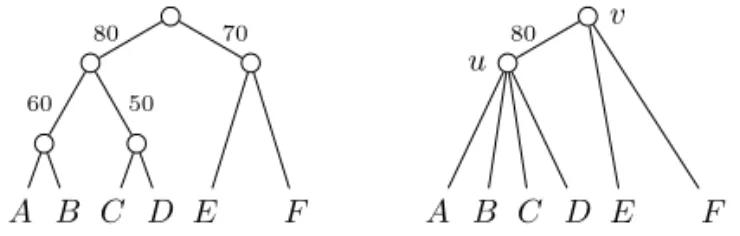
where #T (k) is the number of rooted binary trees with k leaves, i.e. (2k 3)!!. For example, given the trees in Figure 1, the support of the clade {C, D} is 0.5 (i.e. 50/100), while the support of {A, B, C} (which conflicts with {C, D}) is 0.5 · 1
4 = 18 (note that g({C, D}) =
g({A, B, C}) =153).
Frequency of tripartitions. Let ⇡ = (C1,{C2, C3}) be a tripartition.
Let BR(G)1 be the set of binary resolutions of G that generate C1
and let G1 = G \ BR(G)1 be the part of our imaginary sample
whose trees generate C1. If ⇡ 2 ⇧(GB), we define f(⇡) :=
min(f (C1), f (C2), f (C3)). Otherwise, either GB generates C1and
a tripartition ⇡0on the same domain C1as ⇡, or GBdoes not generate
C1. In the first case, we use the knowledge of the frequency of ⇡0and C1
to infer the frequency of ⇡ in our imaginary sample by assuming that the ratio of trees generating ⇡ to trees not generating ⇡0is the same in G1as
in BR(G)1. Thus, f(⇡) := (f(C1) f (⇡0))· ˆg(⇡)/(g(C1) ˆg(⇡0)),
where ˆg(⇡) is the frequency of ⇡ in BR(G). In the second case, we assume that the frequency of trees generating ⇡ is the same in G1as in BR(G)1.
Thus, f(⇡) := f(C1)· ˆg(⇡)/g(C1), where ˆg(⇡) is the frequency of ⇡
in BR(G).
The frequencies ˆgcan be computed as follows. If ⇡ = (C1,{C2, C3})
is generated by u, then we denote by n(Ci)the number of children of u
whose clades are contained in Ci. We define ˆg(⇡) as
#T (n(C2))· #T (n(C3))· #T (n(u) (n(C2) + n(C3)) + 1)
#T (n(u)) .
2 Note that supports have to be numbers between 0 and 1, and thus
bootstrap values should be divided by the size of the bootstrap sample.
80 70 60
A B
50C D E
F
v
u
80A B C D E
F
Fig. 1. A binary gene treeGB(left) and a non-binary one (right) obtained fromGBby
suppressing edges with a support lower than 80.
For example, given the trees in Figure 1, we have the following: f (({A, B, C, D}, {{A, B}, {C, D}})) = 0.5,
f (({A, B, C, D}, {{A, C}, {B, D}})) = 0.3 · 1/14 and f (({A, B, C}, {{B, C}, {A}}) = 1/8 · 1/3.
Finally, conditional clade probability and reconciliation cost can be combined by weighting their ratio (see Scornavacca et al. (2015)).
cjoint(G0, S) = cDTL(G0, S) + cANA(G0)
where G0 is a gene tree in BR(G) and the parameter cAweights the
“sequence contribution" NA(G0) := log (PCCP(G0)))Formally, we
have the following problem:
Problem 4. Polytomy Solver with CCPs under the DTL framework Instance: a dated binary species tree S, a gene tree G, costs , ⌧, respectively for D, T, L events
Output: a binary resolution G0of G minimizing cjoint(G0, S)
Note that Problems 2 and 4 coincide when cA= 0. In experiments with
real-world data, choosing cA> 0gives better results (Scornavacca et al.,
2015), so we used such a joint score in the experiments (see Section 4).
3.2 Unrooted gene trees
Phylogenetic trees are always rooted, but often the position of the root is unknown. The method in the previous section can be used on an unrooted gene tree G to account for the uncertainty on the position of the root, without additional complexity as follows. First, we call Gr the rooted
tree obtained by rooting G arbitrarily on an internal edge e, and GB r
the rooted version of GB, also rooted on e. Then we compute the set
⇧(Gr)of tripartitions as defined in Section 2.3. To obtain ⇧(G), we also
consider, for each non-trivial tripartition (C1,{C2, C3}) 2 ⇧(Gr), the
two other possible tripartitions on L(G) that are implied by a different placement of the root, namely ((L(G) \ C1)[ C2,{L(G) \ C1, C2})
and ((L(G) \ C1)[ C3,{L(G) \ C1, C3}). To these tripartitions, we
add the set ⇧0:={(L(G), {{l}, L(G) \ {l}})|l 2 L(G)} of all trivial
tripartitions.
Each edge e = (u, v) of the rooted binary tree GB
r induces two clades
Cu(e)and Cv(e), which correspond to the label sets of the leaves of the
two subtrees created by removing e. We say that Cu(e)is generated by
uand Cv(e)by v, and we associate to them the support of e. Then, we
redefine the set C(GB
r)as the set of clades induced by all edges of GBr.
Given the set C(GB
r)defined in this way, the support of each clade of
C(Gr)is then computed as in the rooted case.
Finally, we describe how to give a support value to each tripartition of Gin the unrooted case: The support of each tripartition ⇡ 2 ⇧(Gr)is
computed w.r.t. GB
r as described in the previous section, and the support of
the two other possible tripartitions on L(G) that are implied by a different placement of the root is the same as the support of ⇡. All tripartitions in ⇧0have support equal to 1.
3.3 An undated variant
The method discussed by Scornavacca et al. (2015) has been conceived for dated binary species trees, but can easily be adapted to undated ones, while respecting all previously mentioned results, with a slight correction concerning the complexity.
Indeed, reconciliations for undated species trees can be computed in O(|S| · |G|) time with an algorithm described by Bansal et al. (2012). Adapting this algorithm to the amalgamation framework can be done by the same technique used to adapt the O(|S|2· |G|)-time algorithm of Doyon
et al. (2010) for dated species trees reconciliation to the amalgamation framework as done in (Jacox et al., 2016). Thus, our result translates to an O(|S| · |G| · |⇧|)-time algorithm – by Lemma 2.3, an O(|S| · |G| · (3k
2k+1))-time algorithm – for undated species trees.
3.4 Adaptive compromise between the amount of
correction and the computational complexity
The threshold for deciding if a branch is well-supported or not is, in principle, user-defined. However, in the experiments, we required that, in the multifurcated tree resulting from the contraction of unsupported branches, an internal node has at most 12 children. This is done to avoid the combinatorial explosion and to keep the method fast. So we adopted a strategy of increasing the threshold until the 12 maximum children property was satisfied.
4 Application on simulated and biological data
In this section, we use three different data sets, two simulated and one from microbial genomes, to compare the performance of our algorithm with seven different gene tree reconstruction methods: TERA (Scornavacca et al., 2015), ALE (Szöll˝osi et al., 2013), TreeFix-DTL (Bansal et al., 2014), MowgliNNI (Nguyen et al., 2013), JPrIME-DLTRS (Sjöstrand et al., 2014), RAxML (Stamatakis, 2014) and PhyML (Guindon et al., 2010). The first five use information from the sequences and the species tree, while the last two use only information from the sequences. The method described in this paper has been integrated to the ecceTERA package and thus it is called ecceTERA in the comparisons. TERA has also been implemented in the same package, but it is a different method, described in (Scornavacca et al., 2015). The method presented by Kordi and Bansal (2016) has not been tested because no implementation was available at the time of writing. However, as it also solves Problem 2 (with a higher time complexity than our method), it will give the same results as our method for cA= 0, but with a higher running time.
4.1 Simulated Proteobacteria Data Set
The proteobacteria data set is the one constructed to test MowgliNNI and made available by Nguyen et al. (2013). Starting with a dated phylogeny of 37 proteobacteria (David and Alm, 2011):
•1000 evolutionary histories comprising D, T, and L events were
simulated along the species tree according to a birth and death process;
•sequences were simulated along these true gene trees under the GTR
(General Time Reversible) model using Seq-Gen (Rambaut and Grass, 1997);
•RAxML (Stamatakis, 2014) was used to estimate gene trees (along with
100 bootstrap trees) from these sequences under the GTR model. We refer to the section “Simulated gene trees and evolutionary histories” of Nguyen et al. (2013) for more details on how the data set was composed. Some of the test results are taken from the same procedure proposed by Scornavacca et al. (2015).
8 s
37 m
0.4 s 2.5 m 15 s 72 m
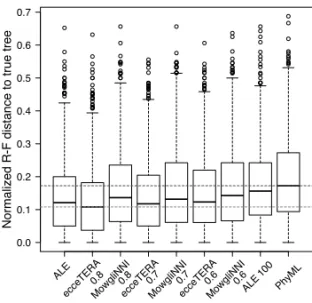
Fig. 2. Accuracy of several methods on the simulated proteobacteria data set: we measure
the normalized Robinson-Foulds distance of the reconstructed tree to the true gene tree for all 1000 gene trees, for 7 methods. Computing times – except for the computation of the RAxML trees – are given in the boxes (s=seconds, m=minutes). In terms of quality, TreeFix-DTL achieves the best accuracy but is relatively slow. ecceTERA is comparable with the second best methods, both in accuracy and computing time.
We ran TreeFix-DTL with default parameters, GTR with a gamma distribution as models of evolution, and as a starting tree the RAxML tree. The RAxML tree (with bootstrap values) was also the input given to MowgliNNI and ecceTERA that were run with a threshold for weak edges equal to 70. As in Scornavacca et al. (2015), JPrIME-DLTRS was run on the sequence alignments with JC69 with a gamma distribution as model of evolution (GTR is not available in JPrIME-DLTRS), 100 000 iterations, a thinning factor of 10 and a time out of 10h. Finally, TERA and ALE were run on the set of bootstrap trees with default parameters, except for the weight of amalgamation cA, fixed to 0.1 for TERA as for ecceTERA.
The accuracy – defined as normalized Robinson-Foulds distance to the true gene tree – of TERA, ecceTERA and ALE is comparable and higher than the one of JPrIME-DLTRS and RAxML (see Figure 2). The method that outperforms the others in this case is TreeFix-DTL. This is possibly due to the fact that the synthetic data set was simulated on the same model used to estimate the gene trees with TreeFix-DTL, making the task easier for the method. Another reason may be the fact that TreeFix-DTL can show signs of significant overfitting of the species tree (Scornavacca et al., 2015). Note also that TreeFix-DTL is slower than ecceTERA, with an average runtime of 37 minutes versus 15 seconds. Interestingly, the accuracy of ecceTERA does not vary if we consider the species tree as undated, while the average runtime decreases considerably (6 seconds).
Note that the normalized Robinson-Foulds distance is not fined-grained and it is not necessarily correlated with reconciliation measures, as noted by Zheng and Zhang (2014a). This is why we also compared trees using the (more fine-grained) normalized triplet distance, with similar results (see Figure 1 of the Appendix).
We also counted the number of genes present in ancestral species according to reconciled gene trees. All gene trees, reconstructed from different methods, are reconciled with TERA to have access to the ancestral gene content, considering trees as rooted for all methods but RAxML (RAxML is the only method tested here that outputs unrooted gene trees). We compared it with the number of genes present in extant species. The results are shown in Figure 3.
Fig. 3. Number of genes for extant species (“Extant"), or ancestral species reconstructed
with reconciled real trees (“Real") or inferred trees from several methods (the others).
Fig. 4. Accuracy of some methods on the sim. cyanobacteria data set. The accuracy of
TERA, TreeFix-DTL and JPrIME-DLTRS are depicted in Figure 2(a) of Scornavacca et al. (2015).
We see that the genome histories are close to the ones inferred from the real trees according to ecceTERA trees, ALE being equivalent in this view. Note that gene trees reconstructed from RAxML only do not yield a correct ancestral genome content. This result argues for the correction step, quickly achieved by ecceTERA, for every evolutionary study.
4.2 Cyanobacteria Data sets
The biological and simulated cyanobacteria data sets used here have been made public by Szöll˝osi et al. (2013) at http://datadryad.org/ resource/doi:10.5061/dryad.pv6df. Their construction con-sisted in selecting 1099 gene families from 36 cyanobacteria species, related by a known dated species tree. These families were retrieved from HOGENOM (Penel et al., 2009), and selected for their reasonable size and representativity. To obtain the biological data set, multiple-alignments on these families were computed with Muscle (Edgar, 2004).
To obtain the simulated data set, from each multiple-alignment of the real data set, a sample of 1000 trees was computed with PhyloBayes (Lartillot et al., 2009), and an amalgamated tree was
reconstructed with ALE (Szöll˝osi et al., 2013). This tree was used to simulate multiple-alignments of artificial sequences evolved along this tree under an LG model with a gamma distribution. This multiple-alignment is the input of our simulated data set. See (Szöll˝osi et al., 2013) for more detail on how the data sets were generated.
Tests on the simulated data set. A tree was computed for each simulated multiple-alignment using PhyML (Guindon et al., 2010), with an LG+ 4+I model and SH branch supports.
For this data set, the accuracy of TERA, ALE, TreeFix-DTL, MowgliNNI, JPrIME-DLTRS and PhyML were compared by Scornavacca et al. (2015, Figure 2(a)) (See Section 2.5 of the same paper for more details on the input/parameters used to generate the results), TERA and ALE giving the best results. In Figure 4, we compare these results with those of ecceTERA, again on unrooted gene trees and dated species tree, for three different thresholds of weakly supported edges (0.8, 0.7 and 0.6). We report the results of ALE and PhyML from Scornavacca et al. (2015), plus the results for MowgliNNI for the same thresholds used for ecceTERA. Both ecceTERA and Mowgli were given the “simulated” PhyML trees with SH branch supports. Finally, we report the accuracy of ALE when using as input 100 sample trees (ALE 100 in Figure 4) among the 10k trees provided, mimicking the information contained in a set of bootstrap trees. Figure 4 shows that, for this data set, ecceTERA with a threshold of 0.8 achieves a slightly better accuracy than all other methods, while with a threshold of 0.7-0.6 the accuracy is comparable to that of ALE. Moreover, the accuracy of ecceTERA increases with the threshold for weak edges, while this is not the case for MowgliNNI. It is also worth noting that the accuracy of ALE decreases considerably when used on small samples of trees. These results are even more interesting when considering that ecceTERA is the fastest method of the bundle (see Table 1 and Figure 2(a) of (Scornavacca et al., 2015)). Although ecceTERA has similar running times as TERA, it requires much less time to construct the input (as its input is the PhyML tree with SH branch supports). Thus, the ecceTERA strategy is the fastest (considering computation + input preparation time) among all compared strategies.Again, comparing the trees using the normalized triplet distance yielded similar results (see Figure 2 of the Appendix). Note that scoring tripartions as described in Section 3.1 and the choice of the costs have impact on the accuracy: running ecceTERA with unitary costs for D, T, L events yields to an average normalized R-F distance of 0.134 for a threshold of 0.8 for weakly supported edges (the average is 0.24 if the costs are respectively 2,3 and 1, see Figure 4); the average stays at 0.133 if the costs are 2,3 and 1 but all tripartitions are considered equiprobable, while it goes down to 0.151 for unitary costs and equiprobable tripartitions.
Tests on the biological data set. From each multiple alignment, a maximum-likelihood tree was computed with PhyML (Guindon et al., 2010) with SH branch supports. These PhyML trees were corrected using ecceTERA with a threshold for weak edges equal to 0.8. The weight of amalgamation cAwas estimated, with starting value 1. Gene trees were
considered as unrooted and the species tree as dated.
We measured the quality of the corrected trees compared to that of the maximum-likelihood trees in two ways. First, we compared the likelihoods according to the multiple-alignments. Of course, the PhyML trees always have a better likelihood because they are optimized with respect to this criterion. But it is interesting to note that for 80% of the trees, an Approximate Unbiased (AU) test performed with Consel (Shimodaira and Hasegawa, 2001) did not reject the ecceTERA tree. So, in a vast majority of the cases, the ecceTERA and PhyML trees are equivalent regarding their sequence likelihoods.
Second, we compared the two sets of trees with respect to their implications for the evolutionary dynamics of genomes: we counted the
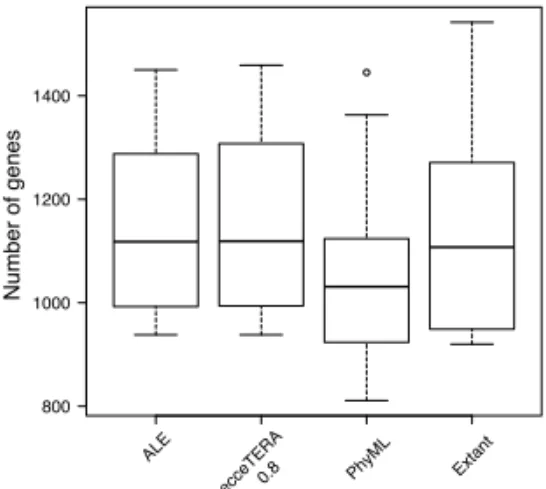
Fig. 5. Number of genes for extant species (“Extant"), or ancestral species reconstructed
with reconciled trees from ALE, ecceTERA and PhyML. Better trees yield more plausible genome histories.
number of genes present in ancestral species according to reconciled gene trees (again all gene trees were reconciled a posteriori with TERA, considering gene trees as rooted for ALE and ecceTERA, and unrooted for PhyML), and compared it with the number of genes present in extant species. The results are shown in Figure 5.
Genome histories are much more stable according to ecceTERA and, equivalently, ALE. According to PhyML trees, ancestral genomes were much smaller than extant genomes, which is not a plausible hypothesis, regarding the theoretical performances of sequence-based constructions, and regarding the same study on simulated genomes (Figure 5).
All results tend to show that the gene tree quality is comparable to that of the best available methods, ALE, TERA and TreeFix-DTL, while solving exactly the non binary gene tree species tree reconciliation, being faster and simpler to use.
5 Conclusions
Gene trees are a precious resource for biologists. They allow us to annotate genomes, to define species taxonomies, and to understand the evolution of traits, adaptation, and modes of genome evolution. They are also used to reconstruct ancestral genomes and understand the history of relations between organisms and their environment on a long time scale. Thus, reliable gene trees are crucial for many biological results (see for example Groussin et al. (2015)).
Standard tools constructing gene trees from multiple sequence alignments are widely used. Although species tree aware methods provide better quality gene trees, they have not been as popular. First because a species tree is not always available, and second because of the computational investment most methods require to output a gene tree.
We propose a method that can be easily used by biologists to quickly correct the output of a gene tree computed from a multiple sequence alignment, provided that branch supports and a species tree are available. The software is built on an FPT algorithm which is derived from recent advances in gene tree amalgamation principles. Its complexity is single exponential in the maximum degree of the input tree, which reduces to the maximal number of connected branches with low support. What a low support is depends on a threshold chosen by the user. Thus, a compromise between the extent of the correction and the computing time is easily achieved. On all of our data sets, on several dozens of species and several thousand of genes, we arrived quickly at a result that is always significantly better than methods based on multiple sequence alignments
only, and whose quality is equivalent to the computationally more intensive integrated methods.
Acknowledgments
All analyzes were performed on the computing cluster of the Montpellier Bioinformatics Biodiversity (MBB) platform.
Funding
This work was supported by the French Agence Nationale de la Recherche Investissements d’Avenir/ Bioinformatique (10-BINF-01-01, ANR-10-BINF-01-02, Ancestrome).
References
Bansal, M. S., Alm, E. J., and Kellis, M. (2012). Efficient algorithms for the reconciliation problem with gene duplication, horizontal transfer and loss. Bioinformatics,28(12), i283–i291.
Bansal, M. S., Wu, Y.-C., Alm, E. J., and Kellis, M. (2014). Improved gene tree reconstruction for deciphering microbial evolution. Submitted. Chang, W.-C. and Eulenstein, O. (2006). Reconciling gene trees with apparent polytomies. In International Computing and Combinatorics Conference, volume 4112 of LNSC, pages 235–244. Springer Berlin Heidelberg.
David, L. A. and Alm, E. J. (2011). Rapid evolutionary innovation during an archaean genetic expansion. Nature,469(7328), 93–96.
Doyon, J.-P., Scornavacca, C., Gorbunov, K. Y., Szöllosi, G. J., Ranwez, V., and Berry, V. (2010). An Efficient Algorithm for Gene/Species Trees Parsimonious Reconciliation with Losses, Duplications and Transfers. In RECOMB International Workshop on Comparative Genomics, volume 6398 of LNBI, pages 93–108. Springer Berlin Heidelberg.
Edgar, R. C. (2004). Muscle: a multiple sequence alignment method with reduced time and space complexity. BMC Bioinformatics,5, 113. Felsenstein, J. (2004). Inferring phylogenies. Sinauer associates
Sunderland.
Groussin, M., Hobbs, J. K., Szöll˝osi, G. J., Gribaldo, S., Arcus, V. L., and Gouy, M. (2015). Toward more accurate ancestral protein genotype-phenotype reconstructions with the use of species tree-aware gene trees. Molecular Biology and Evolution,32(1), 13–22.
Guindon, S., Dufayard, J.-F., Lefort, V., Anisimova, M., Hordijk, W., and Gascuel, O. (2010). New algorithms and methods to estimate maximum-likelihood phylogenies: assessing the performance of PhyML 3.0. Systematic Biology,59(3), 307–321.
Höhna, S. and Drummond, A. J. (2012). Guided tree topology proposals for Bayesian phylogenetic inference. Systematic Biology,61(1), 1–11. Jacox, E., Chauve, C., Szöll˝osi, G. J., Ponty, Y., and Scornavacca, C.
(2016). ecceTERA: Comprehensive gene tree-species tree reconciliation using parsimony. Bioinformatics.
Kordi, M. and Bansal, M. S. (2015). On the complexity of duplication-transfer-loss reconciliation with non-binary gene trees. In International Symposium on Bioinformatics Research and Applications, volume 9096 of LNCS, pages 187–198. Springer International Publishing.
Kordi, M. and Bansal, M. S. (2016). Exact algorithms for duplication-transfer-loss reconciliation with non-binary gene trees. In ACM Conference on Bioinformatics, Computational Biology, and Health Informatics (ACM-BCB), pages 285–294.
Lartillot, N., Lepage, T., and Blanquart, S. (2009). PhyloBayes 3: a Bayesian software package for phylogenetic reconstruction and molecular dating. Bioinformatics,25(17), 2286–2288.
Mossel, E. and Steel, M. (2005). How much can evolved characters tell us about the tree that generated them? In O. Gascuel, editor, Mathematics of Evolution and Phylogeny, pages 384–412. Oxford University Press. Nguyen, T. H., Ranwez, V., Pointet, S., Chifolleau, A.-M. A., Doyon, J.-P.,
and Berry, V. (2013). Reconciliation and local gene tree rearrangement can be of mutual profit. Algorithms for Molecular Biology,8(1), 1. Noutahi, E., Semeria, M., Lafond, M., Seguin, J., Boussau, B., Guéguen,
L., El-Mabrouk, N., and Tannier, E. (2016). Efficient gene tree correction guided by genome evolution. PLoS ONE,11(8), e0159559.
Penel, S., Arigon, A.-M., Dufayard, J.-F., Sertier, A.-S., Daubin, V., Duret, L., Gouy, M., and Perrière, G. (2009). Databases of homologous gene families for comparative genomics. BMC Bioinformatics,10(6), S3. Rambaut, A. and Grass, N. C. (1997). Seq-Gen: an application for the
monte carlo simulation of dna sequence evolution along phylogenetic trees. Computer applications in the biosciences: CABIOS,13(3), 235– 238.
Scornavacca, C., Jacox, E., and Szöllosi, G. J. (2015). Joint amalgamation of most parsimonious reconciled gene trees. Bioinformatics,31(6), 841– 848.
Shimodaira, H. and Hasegawa, M. (2001). CONSEL: for assessing the confidence of phylogenetic tree selection. Bioinformatics,17(12), 1246– 1247.
Sjöstrand, J., Tofigh, A., Daubin, V., Arvestad, L., Sennblad, B., and Lagergren, J. (2014). A Bayesian method for analyzing lateral gene transfer. Systematic Biology,63(3), 409–20.
Stamatakis, A. (2014). RAxML version 8: a tool for phylogenetic analysis and post-analysis of large phylogenies. Bioinformatics,30(9), 1312– 1313.
Szöll˝osi, G. J., Rosikiewicz, W., Boussau, B., Tannier, E., and Daubin, V. (2013). Efficient exploration of the space of reconciled gene trees. Systematic Biology,62(6), 901–912.
Szöll˝osi, G. J., Tannier, E., Daubin, V., and Boussau, B. (2015). The inference of gene trees with species trees. Systematic Biology,64(1), e42–e62.
Zheng, Y. and Zhang, L. (2014a). Are the duplication cost and robinson-foulds distance equivalent? Journal of Computational Biology,21(8), 578–590.
Zheng, Y. and Zhang, L. (2014b). Reconciliation with non-binary gene trees revisited. In International Conference on Research in Computational Molecular Biology, volume 8394 of LNSC, pages 418–432. Springer.