HAL Id: hal-01678423
https://hal.archives-ouvertes.fr/hal-01678423
Submitted on 19 Jan 2021
HAL is a multi-disciplinary open access
archive for the deposit and dissemination of
sci-entific research documents, whether they are
pub-lished or not. The documents may come from
teaching and research institutions in France or
abroad, or from public or private research centers.
L’archive ouverte pluridisciplinaire HAL, est
destinée au dépôt et à la diffusion de documents
scientifiques de niveau recherche, publiés ou non,
émanant des établissements d’enseignement et de
recherche français ou étrangers, des laboratoires
publics ou privés.
Characterization of star-forming dwarf galaxies at 0.1 �z
� 0.9 in VUDS: probing the low-mass end of the
mass-metallicity relation
D. Maccagni, L. Pentericci, D. Schaerer, M. Talia, L. A. M. Tasca, E. Zucca,
A. Calabro, R. Amorin, A. Fontana, E. Perez-montero, et al.
To cite this version:
D. Maccagni, L. Pentericci, D. Schaerer, M. Talia, L. A. M. Tasca, et al.. Characterization of
star-forming dwarf galaxies at 0.1 �z � 0.9 in VUDS: probing the low-mass end of the mass-metallicity
relation. Astronomy and Astrophysics - A&A, EDP Sciences, 2017, 601, pp.A95.
�10.1051/0004-6361/201629762�. �hal-01678423�
A&A 601, A95 (2017) DOI:10.1051/0004-6361/201629762 c ESO 2017
Astronomy
&
Astrophysics
Characterization of star-forming dwarf galaxies at 0.1
<
∼
z
<
∼
0.9
in VUDS: probing the low-mass end of the mass-metallicity
relation
?
A. Calabrò
1, 2, R. Amorín
1, 3, 4, A. Fontana
1, E. Pérez-Montero
12, B. C. Lemaux
13, B. Ribeiro
5, S. Bardelli
8,
M. Castellano
1, T. Contini
9, 10, S. De Barros
11, B. Garilli
6, A. Grazian
1, L. Guaita
1, N. P. Hathi
5, 14,
A. M. Koekemoer
14, O. Le Fèvre
5, D. Maccagni
6, L. Pentericci
1, D. Schaerer
11, 9, M. Talia
7,
L. A. M. Tasca
5, and E. Zucca
81 INAF–Osservatorio Astronomico di Roma, via di Frascati 33, 00040 Monte Porzio Catone, Italy
2 Laboratoire AIM-Paris-Saclay, CEA/DSM-CNRS-Université Paris Diderot, Irfu/Service d’ Astrophysique, CEA Saclay,
Orme des Merisiers, 91191 Gif sur Yvette, France e-mail: antonello.calabro@cea.fr
3 Cavendish Laboratory, University of Cambridge, 19 JJ Thomson Avenue, Cambridge, CB3 0HE, UK 4 Kavli Institute for Cosmology, University of Cambridge, Madingley Road, Cambridge CB3 0HA, UK
5 Aix-Marseille Université, CNRS, LAM (Laboratoire d’Astrophysique de Marseille) UMR 7326, 13388 Marseille, France 6 INAF–IASF, via Bassini 15, 20133 Milano, Italy
7 University of Bologna, Department of Physics and Astronomy (DIFA), viale Berti Pichat 6/2, 40127 Bologna, Italy 8 INAF–Osservatorio Astronomico di Bologna, via Ranzani 1, 40127 Bologna, Italy
9 IRAP, Institut de Recherche en Astrophysique et Planétologie, CNRS, 14 avenue Édouard Belin, 31400 Toulouse, France 10 Université de Toulouse, UPS-OMP, 31400 Toulouse, France
11 Geneva Observatory, University of Geneva, ch. des Maillettes 51, 1290 Versoix, Switzerland 12 Instituto de Astrofísica de Andalucía. CSIC. Apartado de correos 3004, 18080 Granada, Spain 13 Department of Physics, University of California, Davis, One Shields Ave., Davis, CA 95616, USA 14 Space Telescope Science Institute, 3700 San Martin Drive, Baltimore, MD 21218, USA
Received 20 September 2016/ Accepted 15 January 2017
ABSTRACT
Context.The study of statistically significant samples of star-forming dwarf galaxies (SFDGs) at different cosmic epochs is essential for the detailed understanding of galaxy assembly and chemical evolution. However, the main properties of this large population of galaxies at intermediate redshift are still poorly known.
Aims.We present the discovery and spectrophotometric characterization of a large sample of 164 faint (iAB ∼ 23–25 mag) SFDGs
at redshift 0.13 ≤ z ≤ 0.88 selected by the presence of bright optical emission lines in the VIMOS Ultra Deep Survey (VUDS). We investigate their integrated physical properties and ionization conditions, which are used to discuss the low-mass end of the mass-metallicity relation (MZR) and other key scaling relations.
Methods.We use optical VUDS spectra in the COSMOS, VVDS-02h, and ECDF-S fields, as well as deep multi-wavelength photom-etry that includes HST-ACS F814W imaging, to derive stellar masses, extinction-corrected star-formation rates (SFR), and gas-phase metallicities of SFDGs. For the latter, we use the direct method and a Te-consistent approach based on the comparison of a set of
observed emission lines ratios with the predictions of detailed photoionization models.
Results.The VUDS SFDGs are compact (median re∼ 1.2 kpc), low-mass (M∗∼ 107–109 M ) galaxies with a wide range of
star-formation rates (SFR(Hα) ∼ 10−3–101 M
/yr) and morphologies. Overall, they show a broad range of subsolar metallicities (12 +
log(O/H) = 7.26–8.7; 0.04 <∼ Z/Z <∼ 1). Nearly half of the sample are extreme emission-line galaxies (EELGs) characterized by high
equivalent widths and emission line ratios indicative of higher excitation and ionization conditions. The MZR of SFDGs shows a flatter slope compared to previous studies of galaxies in the same mass range and redshift. We find the scatter of the MZR is partly explained in the low mass range by varying specific SFRs and gas fractions amongst the galaxies in our sample. In agreement with recent studies, we find the subclass of EELGs to be systematically offset to lower metallicity compared to SFDGs at a given stellar mass and SFR, suggesting a younger starburst phase. Compared with simple chemical evolution models we find that most SFDGs do not follow the predictions of a “closed-box” model, but those from a gas-regulating model in which gas flows are considered. While strong stellar feedback may produce large-scale outflows favoring the cessation of vigorous star formation and promoting the removal of metals, younger and more metal-poor dwarfs may have recently accreted large amounts of fresh, very metal-poor gas, that is used to fuel current star formation.
Key words. galaxies: evolution – galaxies: high-redshift – galaxies: dwarf – galaxies: abundances – galaxies: starburst
?
Full Tables B.1–B.3 are only available at the CDS via anonymous ftp tocdsarc.u-strasbg.fr (130.79.128.5) or via
http://cdsarc.u-strasbg.fr/viz-bin/qcat?J/A+A/601/A95
1. Introduction
Low-mass (dwarf) galaxies are the most abundant systems of the Universe at all cosmic epochs, as shown by catalogs of nearby
galaxies (Karachentsev et al. 2004) and by the steepness of the galaxy stellar mass (M∗) function at M∗ < 1010 M up to high redshift (Fontana et al. 2006;Santini et al. 2012; Grazian et al. 2015). The most commonly accepted definition of dwarf galax-ies refers to low-mass (M∗ < 109 M ) and low-luminosity sys-tems with Mi− 5 logh100 > −18 (Sánchez-Janssen et al. 2013). They are considered the building blocks from which more mas-sive galaxies form (Press & Schechter 1974). This assembly pro-cess is not constant, but it peaks at z ∼ 2 and then declines expo-nentially at later times (e.g.,Madau & Dickinson 2014). Almost 25% of the stellar mass observed today has been assembled af-ter this peak, and a significant part of it formed in young low-mass galaxies in strong, short-lived starbursts (Guzmán et al. 1997;Kakazu et al. 2007). Some of these star-forming low-mass galaxies also show bright emission lines in their optical rest-frame spectra, due to photoionization of the nebula surrounding hot massive (O type) stars. This makes them easier to identify even beyond the local Universe in current spectroscopic surveys. Throughout this paper, we refer to this kind of faint galaxy with bright emission lines detected in the optical ([O
ii
], [Oiii
], Hβ and Hα) as star-forming dwarf galaxies (SFDG). Among them, a particular subset is represented by extreme emission line galax-ies (EELG), which are selected by the high equivalent width (EW) of their optical emission lines (EW[Oiii
] > 100–200 Å), and have more extreme properties; for example, higher surface densities, lower starburst ages, and lower gas metallicities than the average population of star-forming dwarfs (Kniazev et al. 2004; Cardamone et al. 2009;Amorín et al. 2010,2012,2014,2015; Atek et al. 2011; van der Wel et al. 2011; Maseda et al. 2014). While the population of EELGs itself constitutes an ideal laboratory for studying star formation and chemical enrichment under extreme physical conditions, it also appears to contain en-vironments that most closely resemble “typical” galaxies at very high redshifts (z >∼ 3−4, e.g.,Smit et al. 2014;Stark et al. 2017). Tracing the galaxy-averaged properties of large, represen-tative samples of star-forming dwarf galaxies (SFDGs) since z ∼ 1.5 is a necessary step for gaining a complete understand-ing of the evolution of low-mass galaxies and the build-up of stellar mass during the last 9−10 billion years. How SFDGs as-semble their stellar mass remains one of the unanswered ques-tions surrounding these galaxies. Differently from high-mass (M∗ > 109 M ) galaxies, which show a continuous rate of star formation (SF), the most common scenario for dwarf galaxies is the cyclic bursty mode, as pointed out by theoretical mod-els (e.g., Hopkins et al. 2014; Sparre et al. 2017) and observa-tions (Guo et al. 2016b). Intense SF episodes produce stellar feedback through strong winds and supernova, which heat and expel the surrounding gas in outflows, eventually resulting in a temporary quenching of SF on timescales of tens of Myr (e.g.,Olmo-Garcia et al. 2017;Pelupessy et al. 2004). Then, the metal-enriched gas may be accreted back to the galaxy trig-gering new SF episodes. The scaling relation between stellar mass M∗ and SF rate (SFR = M∗ produced per year) can be used to compare the assembly dynamics of different types of galaxies. For high-mass (M∗ > 109 M ) star-forming galaxies a tight correlation was found between the two quantities at all redshifts from z = 0 to z = 5, called the main sequence (MS) of star-formation (Brinchmann et al. 2004; Noeske et al. 2007;
Daddi et al. 2007;Tasca et al. 2015). This sequence moves to-wards higher SFRs at higher z, though its slope remains almost constant (∼1) (Guo et al. 2015). At lower masses, SFDGs and, in particular, those with the strongest emission lines (EELGs) are found to have increased SFRs at fixed M∗(by ∼1 dex) compared to the extrapolation at low mass of the MS (Amorín et al. 2015),
suggesting that they are efficiently forming stars in strong bursts with stellar mass doubling times <1 Gyr, which cannot be sus-tained for long.
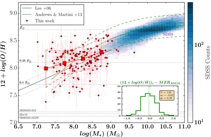
The mechanisms regulating galaxy growth, such as gas ac-cretion and SF feedback are still not completely understood, and the scarcity of direct observations of outflows and gas accretion (as well as a quantification of their rate) represent a limit to a deeper insight (Sánchez Almeida et al. 2014a). However, since the stellar-mass build-up in galaxies is ac-companied by the chemical enrichment of their interstellar medium (ISM), studying the gas-phase metallicity and its re-lation with stellar mass and SFR can help us to investi-gate which of these processes are playing major roles. Thus, the gas-phase metallicity (defined as the oxygen abundance, 12+ log(O/H)) is found to tightly correlate with stellar mass (e.g.,Lequeux et al. 1979;Tremonti et al. 2004) up to high red-shift (z ∼ 3.5, e.g., Maiolino et al. 2008; Zahid et al. 2012a;
Cullen et al. 2014; Troncoso et al. 2014; Onodera et al. 2016), with a relatively steep slope flattening above 1010.5 M . The normalization of this mass-metallicity relation (MZR) appears to evolve to lower metallicities with increasing redshift at fixed stellar mass (Savaglio 2010;Shapley et al. 2005;Erb et al. 2006;
Maiolino et al. 2008; Mannucci et al. 2009), while the slope, especially in its low-mass end, is still not constrained (e.g.,
Christensen et al. 2012;Henry et al. 2013;Whitaker et al. 2014;
Salim et al. 2014). However, both the slope and normalization of the MZR have been found to strongly depend on the method used to derive metallicity (Kewley & Ellison 2008). The largest discrepancies (as high as 0.7 dex) are between metallicities mea-sured using the direct method and strong line methods. The for-mer is also known as the Te method, because it is based on measurement of the electron temperature (Te) of the ionized gas, which requires measurements of weak auroral lines, such as [O
iii
]λ4363 (e.g.,Hägele et al. 2008;Curti et al. 2017). The lat-ter, instead, are based on empirical or model-based calibrations of bright emission line ratios as a function of metallicity.At lower masses (M∗ < 109 M ), the mass-metallicity re-lation is still not completely characterized. Among the various studies that have tried to investigate whether or not a correla-tion exists at lower masses, Lee et al. (2006) (L06) derived a Te-consistent MZR from 27 nearby (D ≤ 5 Mpc) star-forming dwarf galaxies (down to M∗ ∼ 106 M ), with a low scat-ter (±0.117 dex). Using stacked spectra from the SDSS-DR7,
Andrews & Martini(2013) (AM13) measured Tefrom weak au-roral lines and used the direct method to derive metallicities over approximately 4 decades in stellar mass and study the MZR. They found that the MZR has a sharp increase (O/H ∝ M∗1/2) from log(M∗) = 7.4 to log(M∗) = 8.9 M , and flat-tens at log(M∗)= 8.9 M . Above this value, the MZR derived from the direct method reaches an asymptotic metallicity of 12+ log(O/H) = 8.8. Zahid et al. (2012b) studied the mass-metallicity relation down to 107 M , showing that the scatter increases towards lower stellar masses. In a series of papers,
Ly et al.(2014, 2015,2016b) studied 20, 28 and 66 emission line galaxies, respectively, with stellar masses <109 M out to z ∼0.9. In all cases they reported detection of the O4363 Å au-roral line (and significant upper limits for 98 additional sources), which allow them to derive metallicities and investigate the MZR using the direct method. In their latest work, they find that their MZR is consistent with AM13 at z <∼ 0.3, and evolves toward lower abundances at increasing redshifts. Recently, Guo et al.
(2016a) performed a statistically significant analysis of the MZR at z ∼ 0.5–0.7 down to 108 solar masses using a sample of
1381 galaxies collected from deep surveys, 237 of them with M∗ < 109 M , which implied ∼10 times larger than previous studies at similar stellar masses and redshift. While they do not present O4363 Å detections, their statistical study relies on metallicity estimates using the [O
iii
]λ5007/Hβ line ratio and empirical calibrations (Maiolino et al. 2008). Their MZR has a shallower slope than AM13, which is in agreement with theo-retical predictions incorporating supernova energy-driven winds (Dekel & Woo 2003;Davé et al. 2012;Forbes et al. 2014), and they find an increasing scatter toward lower masses, up to 0.3 dex at M∗∼ 108 M .The correlation between stellar mass and metallicity is a natural consequence of the conversion of gas into stars within galaxies, regulated by gas exchanges with the environment through inflows or outflows, but we still don’t know exactly which processes influence the shape, normalization and scat-ter of this relation. Besides observations, semi-analytical models and cosmological hydrodynamic simulations including chemical evolution have tried to explain the observed MZR. According to Kobayashi et al.(2007) and Spitoni et al.(2010), the galac-tic winds can easily drive metals out of low-mass galaxies due to their lower potential wells. In other studies, dwarf galaxies have longer timescales of conversion (regulated by galactic winds) from gas reservoirs to stars, so they are simply less evolved and less enriched systems (Finlator & Davé 2008). The models proposed by Tassis et al. (2008) introduce a critical density threshold for the activation of star-formation, with-out requiring with-outflows to reduce the star formation efficiency and the metal content. Finally, the observed MZR can be ex-plained assuming accretion of metal-poor gas along filaments from the cosmic web (cold-flows) (e.g.,Dalcanton et al. 2004;
Ceverino et al. 2015;Sánchez Almeida et al. 2014b), for which also indirect evidences have been found in recent observations (Sánchez Almeida et al. 2015).
Lastly, SFDGs are important because among them we find analogs of high redshift galaxies, which typically show high sSFRs, low metallicity, high ionization in terms of [O
iii
]λ5007/ [Oii
]λ3727 and compact sizes (Izotov et al. 2015). Recent work by Stasi´nska et al.(2015) shows that EELGs are characterized by [Oiii
]λ5007/[Oii
]λ3727 > 5, reaching values up to 60 in some of them, allowing radiation to escape and ionize the sur-rounding ISM (Nakajima & Ouchi 2014). Such types of galax-ies at high redshift are thought to significantly contribute to the reionization of the Universe, providing up to 20% of the total ionizing flux at z ∼ 6 (Robertson et al. 2015; Dressler et al.2015). As far as the sizes are concerned, SFDGs selected by strong optical emission lines (in particular [Oiii
]λ5007) are typically small isolated systems with radii of the order of ∼1 kpc (Izotov et al. 2016) and they show irregular morpholo-gies (Amorín et al. 2015).This paper presents a characterization of the main inte-grated physical properties of a large and representative sample of 164 star-forming dwarf galaxies at 0.13 < z < 0.88 drawn from the VIMOS Ultra-Deep Survey1 (VUDS, Le Fèvre et al.
2015). By construction, VUDS has two important advantages compared to previous surveys (e.g., zCOSMOS): (i) its unprece-dented depth due to long integrations, which allows us to probe very faint targets IAB∼ 23−25 at z < 1; and (ii) a large area, cov-ering three deep fields, COSMOS, ECDFS, and VVDS-02h, for which a wealth of ancillary multi-wavelength data is available.
1 Based on data obtained with the European Southern
Observatory Very Large Telescope, Paranal, Chile, under Large Program 185.A-0791.
These advantages are particularly important for the main goal of this paper: to investigate the metallicity and ionization of galax-ies with M∗as low as 107 M and the relation with their stellar mass, star-formation rates, and sizes.
We derive galaxy-averaged metallicity and ionization param-eters for the entire sample using a new robust χ2 minimization code called HII-CHI-mistry (HCm,Pérez-Montero 2014), based on the comparison of detailed photoionization models and ob-served optical line ratios. HCm is particularly efficient because it gives results that are consistent with the direct method in the entire metallicity range spanned by our sample, even in the ab-sence of an auroral line detection (e.g., [O
iii
]λ4363). For most galaxies, we use space-based (HST-ACS) images to study their morphological properties and quantify galaxy sizes, allowing us to compare with other samples of SFDGs and study their impact on the mass-metallicity and the other scaling relations.Our paper is organized as follows. In Sect.2, we describe the parent VUDS sample, the parent photometric catalogs and the SDSS data used in this paper for comparison. In Sect.3, we describe the selection criteria adopted to compile our sample of SFDGs, followed by the details on emission line measurements and AGN removal. In Sect. 4 we describe the main physical properties (stellar masses, star-formation rates, morphology and sizes, metallicity and ionization) of the sample and the method-ology used to derive all of them. In Sect. 5, we present our main results and we study empirical relations between different properties, in particular the mass-metallicity relation. We also compare the results with similar samples of star-forming dwarf galaxies at low and intermediate redshift. In Sect.6, we discuss our results, with the implications on galaxy stellar mass assem-bly. We compare our findings to the predictions of simple chemi-cal evolution models, and provide a sample of Lyman-continuum galaxy candidates for reionization studies. Finally, we show the summary and conclusions in Sect.7, while, in an Appendix, we provide tables with all our measurements and compare the metal-licities derived with HCm with those obtained using well-know strong-line calibrations, and study the effects on the MZR.
Throughout this paper we adopt a standardΛ-CDM cosmo-logy with h= 0.7, Ωm= 0.3 and ΩΛ= 0.7. All EWs are presented in the rest-frame. We adopt 12+ log(O/H) = 8.69 as the solar oxygen abundance (Asplund et al. 2009).
2. Observations
2.1. The parent VUDS sample and redshift measurement VUDS (Le Fèvre et al. 2015) is a spectroscopic redshift sur-vey observing approximately 10 000 galaxies to study the ma-jor phase of galaxy assembly up to redshift z ∼ 6. VUDS is one of the largest programs on the ESO-VLT with 640 h of ob-serving time. The survey covers a total of one square degree in three separate fields to reduce the impact of cosmic variance: the COSMOS field, the extended Chandra Deep Field South (ECDFS), and the VVDS-02h field. All the details about the sur-vey strategy, target selection, data reduction and calibrations, and redshift measurements can be found in Le Fèvre et al. (2015) andTasca et al.(2017). Below we briefly summarize the survey features that are relevant to the present study.
The spectroscopic observations were carried out at the VLT with the VIMOS Multi-Object Spectrograph (MOS), which has a wide field of 224 arcmin2 (Le Fèvre et al. 2003). The spec-trograph is equipped with slits 100 wide and 1000 long, as well as two grisms (LRBLUE and LRRED) covering a wavelength range of 3650 < λ < 9350 Å at uniform spectral resolution of
R = 180 and R = 210, respectively. This allows us to observe the Lyman-α line at λ1215 Å up to redshift z ∼ 6.6, and also Hβ, [O
ii
]λλ3727, 3729, and [Oiii
]λλ4959, 5007 emission lines for galaxies at z <∼ 0.88. The integration time (on-source) is '14 h per target for each grism, which allows us to detect the contin-uum at 8500 Å for iAB= 25, and emission lines with an observed flux limit F= 1.5 × 10⁻¹⁸erg s−1cm−2at S /N ∼ 5.Redshift measurements in VUDS were performed using the EZ code (Garilli et al. 2010), both in automatic and manual modes for each spectrum, supervised independently by two per-sons. Different flags have been assigned to each galaxy accord-ing to the probability of the measurement beaccord-ing correct, with flags 3 and 4 as those with the highest (≥95%) probability of be-ing correct. The overall redshift accuracy is dz/(1+ z) = 0.0005– 0.0007 (or an absolute velocity accuracy of 150–200 km s−1). The redshift distribution of the VUDS parent sample shows the majority of galaxies at redshift zspec> 2, while there is a lower redshift tail peaking at zspec ' 1.5, which represents approxi-mately 20% of the total number of targets.
2.2. The parent photometric catalogs
The three fields of the VUDS survey (COSMOS, ECDFS and VVDS-02h) benefit of plenty of deep multi-wavelength data, which are fundamental in combination with the spectroscopic redshifts in order to derive important physical quantities of galaxies, such as stellar masses, absolute magnitudes, and SED-based star-formation rates.
In the COSMOS field (Scoville et al. 2007), GALEX near-UV (2310 Å) and far-near-UV (1530 Å) magnitudes are available down to mAB = 25.5 (Zamojski et al. 2007). Extensive imag-ing observations were carried out with the Subaru Suprime-Cam in BVgriz broad-bands by Taniguchi et al. (2007) down to iAB ∼ 26.5 mag, as well as with CFHT Megacam in the u-band by Boulade et al. (2003). The ULTRA-VISTA survey acquired very deep near-infrared imaging in the YJHK bands with 5σAB depths of ∼25 in Y and ∼24 in JHK bands.
The ECDFS field has been studied by a wealth of pho-tometric surveys as well. All the photometry in this field is taken from Cardamone et al.(2010), who observed with Sub-aru Suprime-Cam in 18 optical medium-band filters (down to RAB∼ 25.3) as part of the MUSYC survey (Gawiser et al. 2006). They also created a uniform catalog combining their obser-vations with ancillary photometric data available in MUSYC. They comprise UBVRIz0bands fromGawiser et al.(2006), JHK fromTaylor et al.(2009) and Spitzer IRAC photometry (3.6 µm, 4.5 µm, 5.8 µm, 8.0 µm) from the SIMPLE survey (Damen et al. 2011).
The VVDS-02h field was observed with u∗g0r0i0z0filters as part of CFHT Legacy Survey (CFHTLS2) by Cuillandre et al.
(2012), reaching iAB= 25.44. Deep infrared photometry is also available in YJHK bands from WIRCAM at CFHT (Bielby et al. 2012) down to KAB= 24.8, and in the 3.6 µm and 4.5 µm Spitzer bands thanks to the SERVS survey (Mauduit et al. 2012). For the VVDS-02h and the ECDFS fields, GALEX photometry is not available.
In addition, for the COSMOS and ECDFS field, we have HST-ACS images in F814W, F125W, and F160W bands from
Koekemoer et al.(2007). The typical spatial resolution of these images are ∼0.0900 for the F814W band (0.6 kpc at z = 0.6), with a point-source detection limit of 27.2 mag at 5σ. We use
2 Data release and associated documentation available at
http://terapix.iap.fr/cplt/T0007/doc/T0007-doc.html
HST images to derive a morphological classification of our galaxies in Sect.4.4. In contrast, the VVDS-02h field does not have HST coverage. The i0 filter images available from CFHT have a lower, seeing-limited spatial resolution of ∼0.800(5.4 kpc at z= 0.6), implying that the most compact and distant galaxies are not completely resolved in VVDS-02h.
2.3. SDSS data
Throughout this paper we compare our results with those found in the local Universe. For this comparison we use star-forming galaxies coming from the SDSS survey DR7 (Abazajian et al. 2009) and publicly available measurements set by MPA-JHU3.
We select our SDSS sample by having a redshift ranging 0.02 < z < 0.32 and signal-to-noise ratio S/N > 3 in the following emission lines: [O
ii
] λλ3727+ 3729 Å (hereafter [Oii
]3727), Hβ, [Oiii
] λ4959 Å, [Oiii
] λ5007 Å, Hα, [Nii
] λ6584 Å and [Sii
] λ6717+ 6731 Å. The stellar masses are derived fit-ting the photometric data from Stoughton et al. (2002) withBruzual & Charlot (2003) population synthesis models as de-scribed in Kauffmann et al. (2003). The star-formation rates are calculated from Hα luminosities following the method of Brinchmann et al. (2004) and scaled to Chabrier (2003) IMF. They fit ugriz photometry and six emission line fluxes ([O
ii
]3728, Hβ, [Oiii
]4959, [Oiii
]5007, Hα, [Nii
]6584 and [Sii
]6717 requiring all S /N > 3) with Charlot & Longhetti(2001) models. These are a combination ofBruzual & Charlot
(2003) synthetic galaxy SEDs and CLOUDY (Ferland et al. 2013) emission line models, calibrated on the observed ra-tios of a representative sample of spiral, irregular, starburst and HII galaxies in the local Universe. Finally, the gas-phase metallicity for the SDSS-DR7 comparison sample has been obtained by Amorín et al. (2010) using the N2 calibration of
Pérez-Montero & Contini(2009), which was derived using ob-jects with accurate measurements of the electron temperature.
3. Sample selection based on emission lines
3.1. The SFDGs sample selection
In order to define our VUDS sample of SFDGs, we first select in VUDS database4a sample of emission-line galaxies with the
following selection criteria:
1. high confidence redshift (at least 95% probability of the red-shift being correct);
2. Spectroscopic redshift in the range 0.13 < zspec< 0.88 and magnitudes iAB> 23;
3. detection (S /N ≥ 3) of the following emission lines: [O
ii
] λ3727 Å, [Oiii
] λλ4959, 5007 Å, Hβ and/or Hα emis-sion lines (we refer to Sect. 3.2 for the emission-line measurements).The above criteria allow us to select low-luminosity galaxies (Mi≤ −13.5 mag) with at least [O
iii
]5007 Å and [Oii
]3727 Å included in the observed spectral range simultaneously, and de-rive metallicities and star-formation rates (see Sect.4). In more detail, the first and second criteria yielded 302 galaxies in COS-MOS, 300 in VVDS-02h, and 113 in ECDFS fields. After re-trieving all their spectra from the VUDS catalog, we checked them visually, one by one, using IRAF. The final selection and3 http://wwwmpa.mpa-garching.mpg.de/SDSS/DR7/
4 1-d spectra fits files, spectroscopic and photometric informations are
0.0 0.2 0.4 0.6 0.8 1.0 redshift 0 5 10 15 20 25 30 35 40 45 # g a la x ie s
Fig. 1. Redshift distribution of VUDS SFDGs selected from the en-tire catalog applying the criteria described in Sect. 3.1. The galaxies are binned in intervals of 0.1 in z, and the median redshift distribution (zmed= 0.56) is represented with a vertical line.
S/N cut was done measuring the emission lines with the method-ology presented in Sect. 3.2, excluding the galaxy whenever one of the four emission lines mentioned above ([O
ii
]3727, [Oiii
]4959, 5007, Hβ and/or Hα) was not detected (S/N < 3), or appeared contaminated by residual sky emission lines. Applying this procedure, we obtained a final total sample of 168 SFDGs in the redshift range 0.13 < z < 0.88, with median value zmed = 0.56 and a vast majority of the galaxies (54%) concen-trated between 0.5 and 0.8, as can be seen in the histogram in Fig.1.3.2. Emission line measurements
Emission lines fluxes and equivalent widths are measured man-ually on a one-by-one basis using the task splot of IRAF by di-rect integration of the line profile after linear subtraction of the continuum, which is well detected in all cases. Additionally, we also fit the emission lines of the galaxies with a Gaussian pro-file. Results using the two approaches are in very good agree-ment for high S/N emission lines (essentially Hα, Hβ, [O
iii
], and [Oii
]), while some differences are found for strongly asym-metric or very low S/N (∼3−5) lines. However, their fluxes and EWs are still consistent within 1σ uncertainties.We compute uncertainties in the line measurements from the dispersion of values provided by multiple measurements adopting different possible band-passes (free of lines and strong residuals from sky subtraction) for the local continuum deter-mination, which is fitted using a second order polynomial. This approach typically gives larger uncertainties compared to those obtained from the average noise spectrum produced by the data reduction pipeline.
For Balmer lines, the presence of stellar absorption features should also be considered. Even though the faintness of the galaxies does not allow detection of significant absorptions for most of them, we have corrected our measurements upwards by 1 Å in EW of Hγ, Hβ and Hα lines for all galaxies (e.g.,Ly et al. 2014). In any case, our galaxies have relatively large EW of Hα and Hβ lines (EW(Hβ)median= 33 Å) and the measurement errors are always higher than 1 Å (∆[EW(Hβ)]median= 8 Å), therefore, this correction must be negligible for our work. In Fig. 2, we show typical spectra for two strong emission-line galaxies in the sample at low- and intermediate-redshift bins, respectively.
As we have described in Sect.1, a particular class of SFDGs has extreme properties; in particular, a high EW of optical
emission lines. Galaxies with EW(O
iii
) > 100 Å are named ex-treme emission line galaxies (EELGs) according to the defini-tion byAmorín et al.(2015). From our sample, 56% qualify as EELGs (see Fig.3).3.3. Identification of AGNs: diagnostic diagrams
Galaxies showing emission lines in their spectra include a broad variety of astrophysical objects that can be distinguished accord-ing to their excitation mechanisms, that is, thermal (e.g., star formation) or non-thermal (in, e.g., AGN or shocks). AGNs are found in two main categories: broad-line (BL) and narrow-line (NL) AGNs. The former were excluded from the VUDS parent sample before we applied our selection criteria, in order to ex-clude from the sample any clear AGN candidate for which we still need to identify narrow-line AGNs, such as Seyfert 2 and LINERs. To that end, we used both a cross-correlation of our sample of galaxies with the latest catalogs of X-ray sources and a combination of two empirical diagnostic diagrams based on optical emission-line ratios.
In the ECDFS field, we used the catalogs E-CDFS (Lehmer et al. 2005) and Chandra 4MS (Luo et al. 2008; Xue et al. 2012;Cappelluti et al. 2016). Inside this field, we can exclude AGNs of high and intermediate luminosity (i.e., those with Lx ≥ 1043 erg s−1). For the COSMOS field, we use the survey Chandra COSMOS (Elvis et al. 2009; Civano et al. 2012) and XMM-COSMOS (Cappelluti et al. 2009), while for the VVDS-02h field we use the catalogs compiled by Pierre et al. (2004) andChiappetti et al.(2013) from the XMM-LSS survey. Since we have a lower sensitivity for the COSMOS and the VVDS fields compared to the ECDFS field, in those cases we can look for only high luminosity AGNs (Lx≥ 1044 erg s−1). We find no X-ray counterpart for any of our VUDS SFDGs in each field ob-served by the survey.
We inspected the spectra for the presence of very high ion-ization emission lines (e.g., [NeV]λ 3426 Å), very broad com-ponents in the Balmer lines, and/or very red SEDs that could suggest the contribution of an AGN, and we did not find any evidence of them.
Finally, we explored two diagnostic diagrams that are fre-quently used to distinguish between SF, AGN, and galaxies with a combination of different excitation mechanisms (com-posites). We used adaptations of the classical BPT diagram, that is, the diagnostics of [O
iii
]λ5007/Hβ versus [Nii
]λ6583/Hα (Baldwin et al. 1981), allowing galaxy classification when Hα and [Nii
] are no longer observable in optical spectra of interme-diate redshift emission-line galaxies. The diagram in Fig.4(left) was proposed byRola et al.(1997) and compares [Oii
]/Hβ and [Oiii
]/Hβ line ratios. The orange continuous line is the empiri-cal separation (with a 1σ uncertainty of approximately 0.15 dex) derived byLamareille et al.(2004) between two types of emit-ting sources: star-forming systems in the bottom left and AGNs in the upper right part.In Fig. 4 (right), we show the Mass-Excitation (MEx) di-agram, introduced byJuneau et al.(2011), which considers the galaxy stellar mass M∗(see Sect.4.1) instead of the [N
ii
]/Hα ra-tio, which is available only for ten galaxies from our sam-ple. This diagram relies on the correlation between the line ratio [Nii
]/Hα and the gas-phase metallicity in SF galaxies (Kewley & Ellison 2008). The empirical relation between mass and metallicity (Tremonti et al. 2004) provides the physical con-nection between the two quantities. The violet line divides the starburst and AGN regimes and was derived empirically from3500 4000 4500 5000 λrest(˚A) 0 5 10 15 20 0 20 40 60 80 100 120 140 F lu x (1 0 − 1 9e rg s cm − 2s − 1˚ A − 1) [O II ] [N e II I] H γ [O II I] λ 4 3 6 3 [O II I] λ 4 9 5 9 [O II I] λ 5 0 0 7 H β 520420821 3500 4000 4500 5000 5500 6000 6500 λrest(˚A) 0 10 20 30 40 50 600 50 100 150 200 250 300 350 F lu x (1 0 − 1 9e rg s cm − 2s − 1˚ A − 1) [O II ] [N e II I] H γ [O II I] λ 4 3 6 3 [O II I] λ 4 9 5 9 [O II I] λ 5 0 0 7 H β H α [N II ] [S II ]λ λ 6 7 1 6 − 6 7 3 1 520389031
Fig. 2.Observed spectra of two galaxies in VUDS with strong emission lines and faint continuum. The galaxy on the left and right hand side panelsare at redshift z= 0.555 and z = 0.173, respectively. While for the former the Hα line lies outside the wavelength range, for the latter it is still visible in the red part of the spectrum. Dotted lines and labels indicate some of the relevant emission lines detected.
0.5 1.0 1.5 2.0 2.5 3.0 log(EW Hβ) (˚A) 0 5 10 15 20 25 30 35 40 # g a la x ie s
Starbursts total sample, M=1.51
not EELGs, M=1.29 EELGs, M=1.72 1.0 1.5 2.0 2.5 3.0 3.5 4.0 log(EW O5007) (˚A) 0 5 10 15 20 25 30 35 40 # g a la x ie s
EELGs total sample, M=2.06
not EELGs, M=1.79 EELGs, M=2.3
Fig. 3.Distribution of EW(Hβ) and EW(O
iii
) for our sample of galaxies selected in Sect.3.1. We lined the histogram with different colors; red for the EELG fraction (EW(Oiii
) > 100 Å based onAmorín et al. 2015) and blue for the non-EELG subset. We emphasize, with vertical continuous lines, the empirical limits for starburst galaxies (EW(Hβ) > 30 Å based onTerlevich et al.(1991) and EELGs, as well as, with vertical dashed lines, the median distribution for the whole sample (black), and the EELGs (red) and non-EELGs (blue) (the values are given in the legend). The standard deviations of the entire distribution are 0.37 and 0.42 for EW(Hβ) and EW(Oiii
), respectively.−1.0 −0.5 0.0 0.5 1.0 1.5 log (OII/Hβ) −0.5 0.0 0.5 1.0 1.5 lo g (O I I I /H β ) Lamareille, 2004 7 8 9 10 11 log(M∗) (M ⊙) Juneau+2014 AGN Star-forming composite AGN Star-forming
Fig. 4.Left: diagnostic diagram to separate SFG, AGN and composite, comparing [O
ii
]λ3727/Hβ and [Oiii
]λ5007/Hβ. The starburst region is in the bottom-left part, while AGNs lie in upper-right part. The red line is the empirical separation byLamareille et al.(2004) with 0.15 dex uncertainty. Right: MEx diagnostic diagram for our sample of emission-line galaxies. The diagram compares the excitation, that is, the emission line ratio [Oiii
]λ5007/Hβ, and the stellar mass M∗. The violet curve is the empirical separation limit between starburst, AGN, and compositeregions according toJuneau et al.(2014). In both diagrams, we mark, with blue squares, the four galaxies that lie completely (also including the errors) in the AGN region according toLamareille et al.(2004).
SDSS emission-line galaxies byJuneau et al.(2014). Below this line, the MEx diagram is populated by star-forming galaxies whose emission lines are powered by stellar photoionization. For this kind of object, models predict an upper limit in the excitation. In the right-upper part, we find AGNs, while in the right-lower part, the region between the two lines is occupied by galaxies showing both star-forming and AGN emission proper-ties (composite). At intermediate redshift (z ≤ 1.5), star-forming galaxies are consistent with having normal interstellar medium (ISM) properties (Juneau et al. 2011), therefore we can, in prin-ciple, apply this diagnostic for all the galaxies in the sample (z < 0.88). We also caution the reader that in AGNs, the [N
ii
] line does not trace the metallicity (e.g., Osterbrock 1989) and the connection between the BPT and MEx may not be straightfor-ward. Therefore, we should consider the results of the MEx di-agram in combination with other diagnostics that do not suffer from this drawback.We find that all galaxies are consistent with purely star-forming systems according to the MEx diagram ofJuneau et al.
(2014), while four galaxies in the [O
iii
]/Hβ versus [Oii
]/Hβ di-agram clearly fall out of the SF region if we consider the 1σ un-certainty (∼0.2 dex) of the empirical relation byLamareille et al.(2004). In addition, we see a small number of SFDGs with relatively high excitation compared to the empirical limit of
Lamareille et al.(2004). It is worth noting that the excitation of objects above those limits does not necessarily require the power of an active nuclear source. A variety of other mechanisms can mimic the properties of AGN in these diagnostics, such as shocks, supernovae, and their subsequent remnants. Indeed, SFDGs (and in particular EELGs) appear to be the preferred sites for the most powerful supernova explosions (Chen et al. 2013;
Lunnan et al. 2013;Leloudas et al. 2015;Thöne et al. 2015). From the combination of the above diagnostics, we find that four galaxies clearly reside in the AGN region of the [O
iii
]/Hβ versus [Oii
]/Hβ plane ofLamareille et al.(2004), so we exclude them from the following analysis. However, the ex-clusion or inex-clusion of these four possible AGN galaxies does not affect any of the results. Indeed, we find that the SFR, metal-licity, and gas fractions of these four galaxies are consistent with the median values for the rest of the sample of secure star-forming systems.After removing the AGN candidates, the subsequent analy-sis was carried out using 164 SFDGs. The basic information for the galaxies, including redshift and selection magnitude, is pre-sented in TableB.1.
4. Methodology
In Table B.2, which is shown in Appendix B(a complete ver-sion is available at the CDS, we present the selected sample of 164 star-forming dwarf galaxies (SFDG) in VUDS. SFDGs are low-mass (M∗ < 109 M ), low-luminosity (MB > −20 mag) galaxies that are forming stars at present, as suggested by the presence of optical emission lines, coming from the gas pho-toionized by newly born massive (O and B) stars. This table also includes measured fluxes (non-extinction corrected) and uncer-tainties for the most relevant emission lines. These quantities, together with an extended ancillary multiwavelength dataset, are used to derive relevant physical properties of the galaxies, which are presented in Table B.3. In this section, we describe our methodology in detail; we will discuss the results in the fol-lowing section.
4.1. Stellar masses from multiwavelength SED fitting
We derive stellar masses from SED fitting performed on the available multi-wavelength photometric data using the code Le Phare (Ilbert et al. 2006), as described inIlbert et al.
(2013). In brief, the code uses a chi-square minimization routine, fitting, for each galaxy,Bruzual & Charlot(2003) stellar popu-lation synthesis models to all broadband photometric data avail-able in each VUDS field (COSMOS, ECDFS, and VVDS-02h) between GALEX far-UV and Spitzer 4.5 µm band, presented in Sect.2.2. The models include different metallicities (Z = 0.004, Z = 0.008, and solar Z = 0.02), visual reddening ranging 0 < E(B−V)stellar< 0.7 and exponentially declining and delayed star-formation histories (SFH) with nine different τ values from 0.1 to 30 Gyr.
We adopt aChabrier (2003) IMF andCalzetti et al. (2000) extinction law, while the contribution of emission lines to the stellar templates is considered in the SED fitting by using an empirical relation between the UV light and the emission line fluxes, as described in Ilbert et al. (2009). The stellar masses for the entire sample of galaxies are presented in Table B.3. Typical 1σ uncertainties in M∗ are ∼0.2 dex and are obtained from the median of the probability distribution function (PDF). Thus, they do not account for possible systematic error (e.g., IMF variations). Besides M∗, additional physical parameters de-rived from SED fitting used in this paper are the extinction-uncorrected rest-frame magnitudes calculated with the method ofIlbert et al.(2005) and, for a subset of galaxies, stellar extinc-tion E(B − V)stellarand star-formation rates (SFRSED).
4.2. Extinction correction
In order to derive extinction-corrected luminosities, we first ob-tain the logarithmic extinction at Hβ, c(Hβ), from the Balmer decrement. Using either Hα and Hβ lines or Hβ and Hγ when Hα is not available, we use the following formulation,
c(Hβ)1= log Hα/Hβ 2.82 ! / fHα (1) c(Hβ)2= log Hγ/Hβ 0.47 ! / fHγ (2)
where the observed ratios are divided by the theoretical values (Hα/Hβ = 2.82 and Hγ/Hβ = 0.47) and for case B recom-bination with Te = 2 × 10⁴ K, ne = 100 cm−3 following
Amorín et al. (2015); fHα and fHγ are the coefficients corre-sponding to the Cardelli et al. (1989) extinction curve at the wavelength of the Hα and Hγ emission lines ( fHα = 0.313,
fHγ= 0.157), respectively.
For 111 galaxies in our sample, we only have one hydrogen line available or the Hα/Hβ and Hβ/Hγ ratios are below their the-oretical values. In these cases, we derive the gas extinction from the stellar reddening, given by the SED fitting (E(B − V)stellar). The reddening of the stellar and nebular components of a galaxy are generally different, and various relations between the two have been found in previous studies.Calzetti et al.(2000) found that the gaseous reddening is typically higher than reddening in low-redshift starburst galaxies, which are more similar to our sample. They apply the following relation E(B − V)nebular = E(B − V)stellar/0.44. More recently, Reddy et al. (2010) found that choosing E(B − V)nebular= E(B − V)stellaris more appropri-ate for studying z ∼ 2 star-forming galaxies, whileWuyts et al.
(2013) derived a relation for massive star-forming galaxies at 0.7 < z < 1.5: E(B − V)gas= E(B−V)stellar+ E(B−V)extra, where E(B − V)extra= E(B− V)stellar× (0.9 − 0.465 ∗ E(B − V)stellar). The
−2.5−2.0−1.5−1.0−0.5 0.0 0.5 1.0 1.5 log(SF RHα)[M⊙/yr] −2.5 −2.0 −1.5 −1.0 −0.5 0.0 0.5 1.0 1.5 lo g (S F Rs e d )[ M ⊙ / y r ] Extinction Reddy et al. (2010) extinction from Balmer decrement −2.5−2.0−1.5−1.0−0.5 0.0 0.5 1.0 1.5 log(SF RHα)[M⊙/yr] Extinction Wuyts et al. (2013) extinction from Balmer decrement −2.5−2.0−1.5−1.0−0.5 0.0 0.5 1.0 1.5 log(SF RHα)[M⊙/yr] Extinction Calzetti et al. (2000) extinction from Balmer decrement
Fig. 5.Comparison between star-formation rates derived from SED fitting (SFRSED) and from the extinction-corrected Hα luminosity (SFRHα), for
different calculations of the extinction coefficient c(Hβ) for the galaxies without an available Balmer decrement. From left to right: E(B − V)gas=
E(B − V)stellar(Reddy et al. 2010); E(B − V)gas= E(B − V)stellar+ E(B − V)extra(Wuyts et al. 2013); E(B − V)gas= E(B − V)stellar/0.44 (Calzetti et al.
2000). In the last panel, the orange crosses represent the galaxies with Balmer decrement available, for which the SFRHαare consistent with the
SFRSEDand no systematic trend is observed.
latter result indicates that nebular light is more attenuated than the stellar light, but the extra-correction is lower than predicted byCalzetti et al.(2000).
In order to decide which relation between stellar and nebu-lar reddening should be applied to our galaxies, we analyze all three possibilities listed above. We derive star-formation rates (SFR) from extinction-corrected Hα luminosities (SFRHα, see Sect.4.3) and compare them with the SFR derived through SED fitting SFRSED(Fig.5).
We find when using the relation byReddy et al.(2010), the SFRHαare systematically lower than the SFRSED, and the di ffer-ences increase toward higher SFRs where extinction corrections are more severe. Using the relations byWuyts et al.(2013) and
Calzetti et al. (2000), we find a tighter correlation and a better agreement between the two SFR measurements, with the latter having the lowest offset ('−0.08 dex) in the whole range of SFR and the lowest dispersion ('0.32 dex). Repeating the same pro-cedure for the galaxies with extinction derived through Balmer decrement, we see that despite the larger scatter, there is no sys-tematic trend between SED and Hα-based SFRs, supporting the consistency of this method.
Overall, we decided to adopt the extinction derived through the Balmer decrement for those galaxies with at least two hy-drogen lines available. For the remaining galaxies, we used the stellar reddening and the relation byCalzetti et al.(2000); then, following the same paper, we obtained the extinction coe ffi-cient c(Hβ) from the corrected reddening as:
c(Hβ)3= E(B − V) × 0.69. (3)
The extinction from SED fitting is used for 109 galaxies in our sample.
4.3. Star-formation rates from Balmer lines
In order to derive the ongoing star-formation rate of the galaxies (i.e., the star-formation activity in the last 10–20 Myr), we adopt the standard calibration ofKennicutt (1998),
SFR= 7.9 × 10−42L(Hα) [erg s−1] (4)
where L(Hα) is the Hα luminosity, corrected for extinction as de-scribed in the previous section. However, for galaxies at z ≥ 0.42,
Hα is no longer visible in our VIMOS spectra. To overcome this limitation, we estimate the Hα luminosities from Hβ fluxes by assuming the theoretical ratio (Hα/Hβ)0= 2.82, valid for case B recombination. FollowingSantini et al.(2009), the SFR derived this way have been scaled down by a factor of 1.7 in order to be consistent with theChabrier(2003) IMF used throughout this paper.
We note that corrections for slit losses due to the finite size of the slit (100) have already been applied to all the spectra dur-ing the calibration process, and it is as accurate as the observed-frame optical photometry. This allows us to efficiently compare photometric (e.g., stellar masses) and spectroscopic quantities (e.g., SFRHα, metallicity), which are investigated in the follow-ing sections. The consistency between Hα-based and SED-based SFRs, shown in Fig.5, supports this procedure.
Finally, we combine Balmer line-based SFRs with stellar masses in order to compute the specific star-formation rate (sSFR= SFR/M∗).
4.4. Morphology and sizes
We perform a visual classification of our star-forming dwarf galaxies as a first approach studying their morphological prop-erties. The selected galaxies are almost unresolved in ground-based CFHT images, but for most of them (those in COSMOS and ECDFS fields), space-based images are available, as pre-sented in Sect. 2.2. In order to have a homogeneous sample, avoiding strong biases in the classification due to the much lower resolution of CFHT images, we analyze only the galaxies in COSMOS and ECDFS (101 in total). For this subset, we do the classification based on HST-ACS F814W band images.
Galaxies at higher reshifts typically show irregular shapes, therefore we cannot follow the Hubble morphological classifi-cation and instead need to choose ad-hoc criteria. In this pa-per, we divide our galaxy sample into the four morphologi-cal classes defined byAmorín et al.(2015) (A15) for low-mass EELGs (EW([O
iii
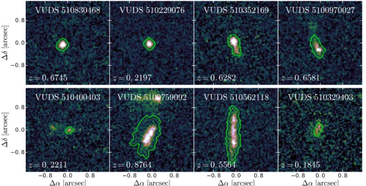
])λ5007 > 100 Å) in our identical red-shift range, applying the criteria also to our non-EELGs. These include Round/Nucleated, Clumpy/Chain, Cometary/Tadpole and Merger/Interacting morphological types. A visual inspectionFig. 6.HST i-band images of eight galaxies in the COSMOS field with different morphological properties. We have: (top line) two round-nucleated galaxies at different redshifts and two cometary-tadpole systems; (bottom line) two interacting-merging galaxies (a faint close galaxy pair and a brighter loose couple), a clumpy-chain system and finally an example of low-surface-brightness dwarf. The stamps are 2 × 2 arcsec wide and the green lines represent the contours of the galaxies.
round-nucleated cometary-tadpole clumpy-chain interacting-merging low SB-unresolved 0 5 10 15 20 # g a la x ie s EELG not-EELG
Fig. 7. Bar histogram showing the number of galaxies falling into each morphological class described in the text for EELG (red) and non-EELG (blue) subsamples. We find that EELGs have a higher fraction of irregular and disturbed morphologies (58%) compared to non-EELGs (34%). Only galaxies in COSMOS and ECDFS fields are considered for this analysis.
of our complete sample of galaxies in COSMOS and ECDFS fields reveals that, following the classification by A15, '40% are round-nucleated, '20% are clumpy-chain, '16% are cometary-tadpole, and '10% are merger-interacting systems, while for the remaining 14% fraction, we cannot determine their morpho-logical type because they appear unresolved or have extremely low surface brightness. As an example, we show (Fig.6) HST F814W images for each galaxy morphological type, while in Fig. 7, we show the distribution of the EELG subsets. Even though there might be inevitable overlap between the last three classes, the latter analysis shows qualitatively that EELGs have, on average, more disturbed morphologies (cometary, clumpy
shapes and interacting-merging systems) compared to non-EELGs, similarly to what was found in A15.
We obtain quantitative morphological parameters for the galaxies in our sample with HST-ACS images available. The analysis was performed using GALFIT (Peng et al. 2002,
2010, version 3.0), following the methodology presented in
Ribeiro et al.(2016), based on recursively fitting a single two-dimensional (2D) Sérsic profile (Sérsic 1968) to the observed light profile of the object. Using this procedure, we obtained the effective radius (semi-major axis) re and the ratio between the observed major and minor axis of the galaxy, q.
We do not deproject re to avoid the introduction of addi-tional uncertainties (given by q), thus we may underestimate the SFR surface density for the most elongated galaxies. However, given the large fraction of round and symmetric galaxies in our sample, we consider the effective radius to be good enough to characterize the size of the objects for our purposes. Further-more, we assume that half of the total star-formation rate (de-rived from Hα luminosity) resides inside the effective radius. This approximation depends on the distribution of the gas rel-ative to the stellar component and can have an opposite effect of deprojection.
Finally, some caveats should be considered when applying GALFIT to our sample. The minimization procedure of the code weighs more the central parts of the object, where the S/N is higher and the nebular emission lines along with young stellar populations contribute the most, inducing an underestimation of the true scale length of the underlying galaxy (Cairós et al. 2007;
Amorín et al. 2007,2009). However, SFDGs (e.g., Blue Com-pact Dwarfs) are usually dominated by nebular emission lines at all radii, and the gas is typically more extended than the central stellar body (Papaderos & Östlin 2012, e.g., IZw18), producing a compensation of the previous effect.
For the galaxies in the VVDS-02h field observed with CFHT, GALFIT does not reach a stable solution in most of the
cases (50%). Even when the fitting code converges, the effective radii suffer from systematic overestimation (difficult to quantify) due to the lower image resolution, as shown in previous VUDS works (Ribeiro et al. 2016). This effect can be especially impor-tant for our dwarf galaxies since they are intrinsically very small, as we illustrate in Sect.5. For these reasons, for the quantitative analysis also, we only consider the galaxies in COSMOS and ECDFS.
4.4.1. Gas fractions and surface densities
We analytically derive SFR surface densities and stellar mass surface densities, dividing SFR and M∗by the projected area of the galaxy by assuming:
ΣSFR= SFR
2 πre2 (5)
ΣM∗=
M∗
2 πre2· (6)
Gas surface density and total gas mass are then computed as-suming that galaxies follow the Kennicutt-Schmidt (KS) law (Kennicutt & Evans 2012) in the form:
ΣSFR= (2.5 ± 0.7) × 10−4 Σgas 1 M pc−2
!1.4±0.15
M yr−1kpc−2. (7) Since this equation assumes a Salpeter IMF, here we have used SFRs consistent with this IMF. Inverting the above relation, we determine the gas surface density:
Σgas= " 0.4 × 10⁴× ΣSFR 1 M yr−1kpc−2 !#0.714 M pc−2. (8) Then, multiplying again by the galaxy area, we derive the total baryonic mass of the gas involved in star formation:
Mgas= Σgas× 2 π(re)2× 10⁶M . (9)
Finally, we derive the gas fractions as: fgas=
Mgas
Mgas+ M∗· (10)
In previous formulae, we have used Salpeter-based SFRs to be consistent with the expression of the KS law (derived as-suming a Salpeter IMF). Likewise, the stellar masses M∗ have been scaled to Salpeter IMF following Bolzonella et al.(2010) (log(M∗)Salp= 0.23 + log(M∗)Chab).
Some caveats should be considered when applying the KS law to our sample. Leroy et al. (2005) show that dwarf galaxies and large spirals exhibit the same relationship be-tween molecular gas and star-formation rate, while Filho et al.
(2016) find that the scatter around the KS law can be very large (∼0.2–0.4 dex) depending on many galaxy properties (e.g., fgas, sSFR). In particular, extremely metal-poor (XMPs) dwarfs (Z < 1/10 Z Kunth & Östlin 2000) tend to fall below the KS relation, having unusually high HI content for theirΣSFRand thus a lower star-formation efficiency. On the other hand, some dwarf galax-ies with enhanced SFR per unit area appear to have higher on-going star-formation efficiency (Amorín et al. 2016). The disper-sion of the KS law, together with the less quantifiable uncertainty in the galaxy sizes, result in fgas errors of at least 0.2−0.3 dex. Given that, the only way to have more reliable and constrained values of fgasandΣgaswould be to measure the gas content di-rectly, such as using CO, dust or [CII] as H2mass tracers.
4.5. Derivation of chemical abundances and ionization parameter
In order to derive the metallicity and ionization parameter for the galaxies in our sample, we used the python code HII-CHI-mistry (HCm). For a detailed description about how this program works, we refer to the original paper byPérez-Montero(2014) (PM14), and summarize here the basic principles.
4.5.1. Te−consistent, model-based abundances
HCm is based on the comparison between a set of observed line ratios and the predictions of photoionization models us-ing CLOUDY (Ferland et al. 2013) and POPSTAR (Mollá et al. 2009). Compared to previous methodologies, the models con-sider all possible ranges of physical properties for our galaxies, including variations of the ionization parameter. This quantity is defined as:
log(U)= Q(H)
4πr2nc (11)
where Q(H) is the number of ionizing photons (λ < 912 Å) in s−1, r is the outer radius of the gas distribution in cm, c is the speed of light in cm/s, and n is the number density of hydrogen in cm−3. The larger the value of log(U), the more ionized the gas, even though collisional ionization can play an important role, especially when the temperature of the gas is high (hundreds of thousands of degrees).
Assuming the typical conditions in gaseous ionized neb-ulae, the grid probes possible values of log(U) in the range [−1.50, −4.00], metallicity 12+ log(O/H) in the range [7.1, 9.1], and log(N/O) between 0 and −2. Using a robust χ2 mini-mization procedure, HCm allows the derivation of three quan-tities: the oxygen abundance (O/H), the nitrogen over oxy-gen abundance (N/O), and the ionization parameter (log(U)), which best reproduce this set of five emission line ratios: [O
ii
]λ3727 Å, [Oiii
]λ4363 Å, [Oiii
]λ5007 Å, [Nii
]λ6584 Å, and [Sii
]λλ6717+ 6731 Å (all relative to Hβ), which are pro-vided as input parameters. The procedure consists of two steps; in the first step a comparison is made between the observed extinction-corrected emission-line intensities and the grid of models, providing a value of N/O. Then, the nitrogen abundance is used to constrain the models and derive reliable oxygen abun-dance and ionization parameters with the same χ2minimization methodology.HCm provides abundances that are consistent with those derived from the direct method for a large range of metalli-city values and for a broad variety of galaxy types in the lo-cal Universe. The agreement between the model-based O/H and N/O abundances and those derived using the direct method is excellent when all the lines are used. Reliable model-based es-timation of O/H can also be obtained without [O
iii
]λ4363 Å detection if a limited grid of models is adopted using an em-pirical relation between log(U) and 12+ log(O/H). The rela-tion between the metallicity and the ionizarela-tion parameter arises from the physical properties of gaseous nebulae. It is con-sistent with large samples of local star-forming galaxies and HII regions (PM14), and has also been tested for the SFDGs in our sample with detected [Oiii
]λ4363 Å lines, in which case no assumptions are made by the code. The role of this rela-tion is to minimize the dispersion in the determinarela-tion of O/H (PM14). Finally, when only [Oii
]λ3727 Å, [Oiii
]λ5007 Å, and Hβ are observed (the code is assuming a typical ratio between [Oiii
]λ5007 Å and [Oiii
]λ4959 Å of 3.0, Osterbrock 1989),7.0 7.5 8.0 8.5 12 + log(O/H) HII-CHI-mistry −0.6 −0.4 −0.2 0.0 0.2 0.4 ∆ (1 2 + lo g (O / H )) 7.0 7.5 8.0 8.5 7.2 7.4 7.6 7.8 8.0 8.2 8.4 12 + lo g( O /H ) d ir ec t m et h o d −0.4−0.2 0.0 0.2 0.4 0 2 4 6 8 10 12 14 ∆(12 + log(O/H)) Tot = 19 Median = 0.01 Std = 0.09
Fig. 8.Comparison between the metallicity derived with the code HCm and the direct method, showing the consistency of our approach. The red dashed line is the 1:1 relation. At the bottom of the figure, the di ffer-ences between the two methods are plotted as a function of the metal-licity. The blue dashed line corresponds to the 0 level, while the blue continuous line is the median value. In the lower-right box, we have added the histogram with the distribution of the differences, with the median value line in green.
the R23 index ([O
ii
]λ3727 Å+ [Oiii
]λλ4959+ 5007 Å)/Hβ is used as a proxy to derive O/H, in combination with the [Oii
]λ3727 Å/[Oiii
]λ5007 Å ratio to partially remove the de-pendence on log(U). This is the most frequent case for our sam-ple, since 93% of our SFDGs without an auroral line detection also have no detected [Nii
]λ6584 and [Sii
]λλ6717, 6731.The procedure described above allows us to apply HCm for galaxies beyond the local Universe, where galaxies are fainter and [O
iii
]λ4363 Å is generally not detected. HCm shows an in-crease of the dispersion (compared to the direct method) when a lower number of emission lines is considered, but gives re-sults that are more consistent with the direct method than other empirical and theoretical calibrations. We find that the system-atic differences with respect to HCm (and the direct method) can be as high as ∼0.7 dex at lower metallicities, depending on the adopted calibration. We refer to Appendix Afor a description of the calibrations analyzed in this paper and a more detailed comparison with our results.4.5.2. Direct method
For a fraction of galaxies in our sample (19), we detect the [O
iii
] λ4363 Å auroral line, which is sensitive to the electron temperature Te. This allows us to use the direct method and check the consistency with metallicities for these galaxies de-rived through HCm. Despite the small number of galaxies, the two methods give consistent results within the errors over the entire metallicity range for the majority of them (Fig. 8). We do not find any systematic trend in the low- or high-Z regime, and the median difference between the two measurements is of 0.01 dex. According to PM14, the consistency between HCm and the direct method, tested for an analogous sample of local star-forming galaxies, is of ∼0.15 dex. In our case, the 1σ scat-ter is of the same order of magnitude (∼0.09 dex); even lower−22 −20 −18 −16 −14 MB − 5l og (h 7 0 ) 0.0 0.2 0.4 0.6 0.8 1.0 redshift 6 7 8 9 10 lo g (M ∗/M ⊙ ) zCOSMOS EELGs VUDS VUDS EELGs
Fig. 9.Top: MB − 5 log h70 vs. redshift for our sample of galaxies
(crosses) and for zCOSMOS EELGs by Amorín et al. (2015) (filled circles), color coded according to different bins of redshift (0.1–0.3, 0.3−0.5, 0.5–0.7 and 0.7–0.9). The EELG fraction of our galaxies is evidenced by empty circles around the crosses. The B-band luminosi-ties span a wide range, −13 ≤ MB ≤ −21.5, increasing with redshift.
Bottom: Galaxy stellar mass vs. redshift for the same galaxy samples.
than the previous value. Thus, we safely apply the code HCm to the other galaxies in the sample without auroral line detection.
5. Results
In this section, we present the properties of the SFDG sample and we study the key scaling relations between them. The main physical quantities presented here are listed in TableB.3.
In Fig. 9, we show that the stellar masses of the galaxies, derived through SED fitting, span a wide range of values from 1010 down to 107 M (median value of 108.2 M ), a region in the stellar mass distribution of galaxies which is still strongly under-represented in current spectroscopic surveys at intermedi-ate redshift. Compared to zCOSMOS EELGs (A15), which is one of the largest samples of low-mass star-forming galaxies at these redshifts (see alsoLy et al. 2016b), we extend the intrinsic luminosity of the sources (given in rest-frame absolute magni-tude MB) down by ∼2 mag thanks to VUDS deeper observations. As a consequence, our sample extends to lower stellar masses, though we are biased toward the higher M∗at a given redshift.
In Fig. 10, we present the distribution of various physical quantities: extinction correction c(Hβ), specific star-formation rate (sSFR), effective radius (re), gas fraction ( fgas), ionization parameter (log(U)) and oxygen abundance (12+ logO/H). The histogram of extinction coefficients shows that the dust extinc-tion is generally low, with median reddening of E(B − V) = 0.45 mag (σ = 0.38), and there is no significant difference be-tween EELG and non-EELG distributions. The reddening values found here are consistent with previous studies on local (e.g., Kniazev 2004) and intermediate-redshift samples of SFDGs (e.g., Amorín et al. 2015; Ly et al. 2014, 2015). Our galaxies have low to moderate SFRs ranging 10−3<∼ SFR <∼ 101M yr−1, with a median SFR= 0.64 M yr−1, and 1σ scatter of 0.6. As a consequence, the sSFR tend to be high, spanning a broad range, 10−10yr−1<
0.0 0.2 0.4 0.6 0.8 1.0 c(Hβ) 0 10 20 30 40 # g a la x ie s total sample, M=0.31 not EELGs, M=0.26 EELGs, M=0.31 −9.5 −9.0 −8.5 −8.0 −7.5 −7.0 log(ssfr) (yr−1) 0 5 10 15 20 25 30 # g a la x ie s total sample, M=-8.51 not EELGs, M=-8.86 EELGs, M=-8.3 −1.0 −0.5 0.0 0.5 1.0 log(re) [kpc] 0 5 10 15 20 # g a la x ie s total sample, M=0.09 not EELGs, M=0.17 EELGs, M=0.06 0.2 0.3 0.4 0.5 0.6 0.7 0.8 0.9 1.0
fgas= Mgas/(Mgas+ M∗)
0 2 4 6 8 10 12 14 # g a la x ie s total sample, M=0.74 not EELGs, M=0.59 EELGs, M=0.81 −3.0 −2.5 −2.0 −1.5 log(U ) 0 5 10 15 20 25 30 35 40 # g a la x ie s total sample, M=-2.67 not EELGs, M=-2.85 EELGs, M=-2.54 7.4 7.6 7.8 8.0 8.2 8.4 8.6 8.8 12 + log(O/H) 0 5 10 15 20 25 30 35 40 # g a la x ie s total sample, M=8.17 not EELGs, M=8.26 EELGs, M=8.09
Fig. 10.Histogram distribution of extinction coefficient c(Hβ), sSFR, and circularized effective radius re(top), gas fraction fgas, gas-phase
metal-licity and ionization parameter log(U) (bottom) for our selected galaxies. The EELG and non-EELG fractions are highlighted with red and blue lines, respectively, filling the histogram. The median distribution values for each quantity are indicated in the legend for each subset of galaxies.
sSFR galaxies. The whole sample has a median of 10−9 yr−1, well above the Milky Way integrated sSFR (∼1.5 × 10⁻¹¹yr−1). We also find that our galaxies are very compact, with e ffec-tive radii (in kpc) in the range 0.1 ≤ re ≤ 6 kpc and median value of re= 1.2 kpc (standard deviation of 2.3 kpc), compara-ble to BCDs (Papaderos et al. 1996;Gil de Paz & Madore 2005;
Amorín et al. 2009) and the Green Pea galaxies (Amorín et al. 2012). In the same figure, we show the distribution of values of the gas fraction of our SFDGs. The values range 0.25 < fgas < 0.95, and the distribution is peaked toward higher fgas, with one half of our galaxies showing fgas> 0.74, that is, more than 74% of the total baryonic mass resides in their gas reservoirs. The highest values are found in EELGs, which show a median fgas∼ 0.2 higher compared to non-EELGs. These results for the whole sample could be an indication that the star-formation efficiency has been very low or that our galaxies are very young and still assembling most of their stellar mass. In the local Universe, such values of gas fractions can be found in low-mass, low-metallicity and highly star-forming galaxies (e.g., Lara-López et al. 2013;
Filho et al. 2016;Amorín et al. 2016).
5.1. The relation between star-formation rate and stellar mass
For high-mass star-forming galaxies (M∗ > 109 M ), a tight correlation has been found between the star-formation rate and the stellar mass (e.g.,Brinchmann et al. 2004;Elbaz et al. 2007;
Tasca et al. 2015) up to redshift 5. This correlation, called the star-formation main sequence (MS), is displaced toward higher values of SFR at higher z, with an almost constant slope of approximately 1 (Guo et al. 2015) and a small non-varying SFR dispersion of ∼0.3 dex (Schreiber et al. 2015). An exten-sion of the MS has been derived by Whitaker et al.(2014) for intermediate-redshift star-forming galaxies (0.5 < z < 1) down
to M∗ ∼ 108 M , but the relation remains poorly constrained at lower masses.
Our sample of 164 VUDS SFDGs allows us to populate the low-mass end of the SFR-M∗relation (Fig.11). Our sample has a higher average SFR per unit mass compared to the extrapola-tion of the MS at low masses (M∗ < 108.4 M ,Whitaker et al.
2014) This result should be considered as a secondary effect of our selection criteria, based on a S /N > 3 cut on hydrogen re-combination lines, [O
ii
]λ3727 and [Oiii
]λ5007 (see Sect.3.1). At a given continuum luminosity and stellar mass, we are limited to the brighter Hα (Hβ) values (i.e., higher sSFRs) compared to a continuum S/N-selected sample. We also notice that a conspic-uous number of SFDGs have higher star-formation rates than the median population, with starburstiness parameters (defined as SFR/SFRMS,Schreiber et al. 2015) up to 1.8 dex, similar to zCOSMOS EELGs.This difference is more evident when we consider the sSFR versus M∗. The sSFR distribution of the EELG fraction is biased high (∼+0.6 dex) with respect to the non-EELGs. We also find that the starburstiness parameter depends on the gas fraction. In particular, the median gas fraction of the sample ( fgas;med= 0.74) is very effective for distinguishing between these two classes, with more gas-rich galaxies having, on average, higher sSFRs (∼1 dex) compared to the MS star-forming population (Fig.12).
5.2. Chemical abundances and ionization properties
In the last two panels of Fig.10, we present the results of the code HCm, the ionization parameter, and the metallicity. We discard, from this analysis, 10 galaxies of our VUDS original sample for which some of the emission lines required by the code are not reliably detected. For the remaining 152 galax-ies, we find that they span a wide range of values, respectively −3.17 < log(U) < −1.55 and 7.26 < 12+ log(O/H) < 8.6.

![Fig. 4. Left: diagnostic diagram to separate SFG, AGN and composite, comparing [O ii ]λ3727/Hβ and [O iii ]λ5007/Hβ](https://thumb-eu.123doks.com/thumbv2/123doknet/14713517.568174/7.892.86.808.801.1066/fig-left-diagnostic-diagram-separate-sfg-composite-comparing.webp)